Special least squares solutions of the reduced biquaternion matrix equation with applications 22footnotemark: 2
Abstract
This paper presents an efficient method for obtaining the least squares Hermitian solutions of the reduced biquaternion matrix equation . The method leverages the real representation of reduced biquaternion matrices. Furthermore, we establish the necessary and sufficient conditions for the existence and uniqueness of the Hermitian solution, along with a general expression for it. Notably, this approach differs from the one previously developed by Yuan et al. , which relied on the complex representation of reduced biquaternion matrices. In contrast, our method exclusively employs real matrices and utilizes real arithmetic operations, resulting in enhanced efficiency. We also apply our developed framework to find the Hermitian solutions for the complex matrix equation , expanding its utility in addressing inverse problems. Specifically, we investigate its effectiveness in addressing partially described inverse eigenvalue problems. Finally, we provide numerical examples to demonstrate the effectiveness of our method and its superiority over the existing approach.
Keywords. Least squares problem, Reduced biquaternion matrix equation, Real representation matrix, Partially described inverse eigenvalue problem.
AMS subject classification. 15B33, 15B57, 65F18, 65F20, 65F45.
1 Introduction
Matrix equations play a vital role in various fields, including computational mathematics, vibration theory, stability analysis, and control theory (for example, [2, 5, 7]). Due to their significant applications in various fields, a substantial amount of research has been dedicated to solving matrix equations. See [8, 9, 15, 17] and references therein. In this paper, we address the following matrix equation:
| (1) |
where , , , , , and are given matrices of appropriate sizes, and represents the unknown matrix of an appropriate size. This matrix equation has been extensively studied in the real, complex, and quaternion fields, leading to several important findings. Notably, Liao et al. [10] provided an analytical expression for the least squares solution with the minimum norm in the real field. Ding et al. [3] proposed two iterative algorithms to obtain solutions in the real field. Mitra [11] delved into the necessary and sufficient conditions for the existence of solution and presented a general formulation for the solution in the complex field. Navarra et al. [12] offered a simpler consistency condition and a new representation of the general common solution compared to Mitra [11]. They also derived a representation of the general Hermitian solution for , provided the Hermitian solution exists. Wang et al. [16] determined the least squares Hermitian solution with the minimum norm in the complex field using matrix and vector products. Zhang et al. [22] developed a more efficient method compared to [16] for finding the least squares Hermitian solution with the minimum norm by utilizing the real representation of a complex matrix. Yuan et al. [19] studied the least squares L-structured solutions of quaternion linear matrix equations using the complex representation of quaternion matrices. However, limited research has been conducted on solving matrix equations in the reduced biquaternion domain.
A reduced biquaternion, a type of hypercomplex number, shares with quaternions the characteristic of possessing a real part alongside three imaginary components. However, it distinguishes itself by offering notable advantages over its quaternion counterpart. One significant distinction is the commutative nature of multiplication, which streamlines fundamental operations like multiplication itself, SVD, and eigenvalue calculations [14]. This results in algorithms that are less complex and more expeditious in computational procedures. For instance, Pei et al. [13, 14] and Gai [4] demonstrated that reduced biquaternions outperform conventional quaternions for image and digital signal processing. Despite the advantage of reduced biquaternions over quaternions, limited research has been dedicated to solving reduced biquaternion matrix equations (RBMEs). Recently, Yuan et al. [18] studied the necessary and sufficient conditions for the existence of a Hermitian solution of the RBME (1) and provided a general formulation for the solution by using the method of complex representation (CR) of reduced biquaternion matrices. However, this method involves complex matrices and complex arithmetic, leading to extensive computations.
In the existing literature, several papers have employed the real representation method to solve matrix equations within the complex and quaternion domains. For instance, in [22], the authors utilized real representation of complex matrices to address the complex matrix equation . In [20, 21, 24], similar approaches were taken using real representation of quaternion matrices to tackle quaternion matrix equations. These studies clearly demonstrate the superior efficiency of the real representation (RR) method compared to the complex representation (CR) method when dealing with matrix equations in the complex and quaternion domains. However, the real representation method has not yet been explored in the context of solving reduced biquaternion matrix equations. Motivated by insights from prior research, this paper introduces a more efficient approach for finding the Hermitian solution to RBME (1). Here are the highlights of the work presented in this paper:
-
•
We explore the least squares Hermitian solution with the minimum norm of the RBME (1) using the method of real representation of reduced biquaternion matrices. The notable advantage of this method lies in its exclusive use of real matrices and real arithmetic operations, resulting in enhanced efficiency.
-
•
We establish the necessary and sufficient conditions for the existence and uniqueness of the Hermitian solution to RBME (1) and provide a general form of the solution.
-
•
In light of complex matrix equations being a special case of reduced biquaternion matrix equations, we utilize our developed method to find the Hermitian solution for matrix equation (1) over the complex field.
-
•
We conduct a comparative analysis between the CR and RR methods to study the Hermitian solution of RBME (1).
Furthermore, this paper explores the application of the proposed framework in solving inverse eigenvalue problems. Inverse eigenvalue problems often involve the reconstruction of structured matrices based on given spectral data. When the available spectral data contains only partial information about the eigenpairs, this problem is termed as a partially described inverse eigenvalue problem (PDIEP). In PDIEP, two crucial aspects come to the forefront: the theory of solvability and the development of numerical solution methodologies (as detailed in [1] and related references). In terms of solvability, a significant challenge has been to establish the necessary or sufficient conditions for solvability of PDIEP. On the other hand, numerical solution methods aim to construct matrices in a numerically stable manner when the given spectral data is feasible. In this paper, by leveraging our developed framework, we successfully introduce a numerical solution methodology for PDIEP [1, Problem 5.1], which requires the construction of the Hermitian matrix from an eigenpair set.
The manuscript is organized as follows. In Section 2, notation and preliminary results are presented. Section 3 outlines a framework for solving constrained RBME. Section 4 highlights the application of our developed framework to solve PDIEP. Section 5 offers numerical verification of our developed findings.
2 Notation and preliminaries
2.1 Notation
Throughout this paper, denotes the set of all reduced biquaternions. , , and represent the sets of all real, complex, and reduced biquaternion matrices, respectively. We also denote , , , and as the sets of all real symmetric , real anti-symmetric, complex Hermitian, and reduced biquaternion Hermitian matrices, respectively. For a diagonal matrix , we denote it as , where whenever and for . For , the notations , and stand for the Moore-Penrose generalized inverse, transpose, real part, and imaginary part of , respectively. represents the identity matrix of order . For , denotes the column of the identity matrix . denotes the zero matrix of suitable size. represents the Kronecker product of matrices . The symbol represents the Frobenius norm. represents the -norm or Euclidean norm. For and , the notation represents the matrix .
Matlab command creates an codistributed matrix of normally distributed random numbers whose every element is between and . returns an matrix of uniformly distributed random numbers. and returns an matrix of ones and zeros, respectively. creates a Toeplitz matrix whose first row and first column is . generates an identity matrix of size . Let be any matrix of size . returns the upper triangular part of a matrix , while setting all the elements below the main diagonal to zero. returns the elements on and above the diagonal of , while setting all the elements below it as zero. We use the following abbreviations throughout this paper:
RBME : reduced biquaternion matrix equation, CME : complex matrix equation, CR : complex representation, RR : real representation.
2.2 Preliminaries
A reduced biquaternion can be uniquely expressed as , where for , and , . The norm of is . The Frobenius norm for is defined as follows:
| (2) |
Let , where for . The real representation of matrix , denoted as , is defined as follows:
| (3) |
Let denote the first block row of the block matrix , i.e., We have
| (4) |
For matrix , let . We have . Clearly, the operator is linear, which means that for , , and , we have Also, we have
| (5) |
For , , and , it is well known that . Now, we present two key lemmas. The subsequent lemma can be easily deduced from the structures of and .
Lemma 2.1.
Let , , and . Then the following properties hold.
-
(i)
.
-
(ii)
, , .
-
(iii)
, , .
Lemma 2.2.
Let . Then . We have
| (6) |
where , , , . is a block matrix of size with at the position, and the rest of the entries are zero matrices of size , where and .
The above lemma can be easily derived through direct computation; thus, we omit the proof. To enhance our understanding of the above lemma, we will examine it in the context of . In this scenario, we have
,
,
,
Now, we recall some fundamental results that are pivotal in establishing the main findings of this paper.
Definition 2.3.
For , let , , , , , and denote by the following vector:
| (7) |
Definition 2.4.
For , let , , , , , and denote by the following vector:
| (8) |
Lemma 2.5.
For any , it is easy to see that
Set
| (9) |
Lemma 2.6.
If , then
Proof.
Additionally, we need the following lemma for developing the main results.
Lemma 2.7.
[6] Consider the matrix equation of the form , where and . The following results hold:
-
(i)
The matrix equation has a solution if and only if . In this case, the general solution is where is an arbitrary vector. Furthermore, if the consistency condition is satisfied, then the matrix equation has a unique solution if and only if . In this case, the unique solution is .
-
(ii)
The least squares solutions of the matrix equation can be expressed as where is an arbitrary vector, and the least squares solution with the least norm is .
3 Framework for solving constrained RBME
In this section, we initially investigate the least squares Hermitian solution with the least norm of RBME (1) using the RR method. The problem is formulated as follows:
Problem 3.1.
Given matrices , , and , let
Then, find such that
Next, by utilizing the RR method, we derive the necessary and sufficient conditions for the existence of the Hermitian solution for RBME (1), along with a general formulation for the solution if the consistency criterion is met. We also establish the conditions for a unique solution and, in such cases, provide a general form of the solution. The RR method involves transforming the constrained RBME (1) into an equivalent unconstrained real linear system.
Following that, we present a concise overview of the CR method, which is employed to find the Hermitian solution for RBME (1) as documented in [18]. Additionally, we conduct a comparative analysis between the RR and CR methods.
Before proceeding, we introduce some notations that will be used in the subsequent results. Let
| (10) |
Theorem 3.1.
Proof.
By using (2), (4), and Lemma 2.1, we get
We have
By using Lemma 2.2 and Lemma 2.6, we get
Thus,
Hence, Problem 3.1 can be solved by finding the least squares solutions of the following unconstrained real matrix system:
| (13) |
By using the fact that , and using Lemma 2.5, we have
| (14) |
By using Lemma 2.7, the least squares solutions of matrix equation (13) is given by
| (15) |
where is an arbitrary vector. Hence, we get (11) by utilizing (14) and (15).
Theorem 3.2.
Let and be in the form of (10), and let . Additionally, let and be as in (6) and (9), respectively. Then, the RBME (1) has a Hermitian solution if and only if
| (17) |
In this case, the general solution satisfies
| (18) |
where is an arbitrary vector. Furthermore, if (17) holds, then the RBME (1) has a unique solution if and only if
| (19) |
In this case, the unique solution satisfies
| (20) |
Proof.
By using Lemmas 2.1, 2.2, and 2.6, we have
Hence, solving the constrained RBME (1) is equivalent to solving the following unconstrained real matrix system:
| (21) |
By using the fact that , and using Lemma 2.5, we have
| (22) |
By leveraging Lemma 2.7, we obtain the consistency condition (17). This condition establishes the criterion that ensures a solution to matrix equation (21) and a Hermitian solution for RBME (1). In this case, the solution to matrix equation (21) can be expressed as
| (23) |
where is an arbitrary vector. By applying (22) and (23), we get that the Hermitian solution to RBME (1) satisfies (18).
Furthermore, if condition (17) is satisfied, applying Lemma 2.7 leads to the derivation of the condition (19). This condition signifies the criterion for ensuring a unique solution to matrix equation (21) and a unique Hermitian solution to RBME (1). In this case, the unique solution to matrix equation (21) is given by
| (24) |
By using (22) and (24), we get that the unique Hermitian solution to RBME (1) satisfies (20). ∎
In [18], the authors investigated the Hermitian solution of RBME (1) using the CR method. They successfully established the necessary and sufficient conditions for the existence of a solution, along with providing a general expression for it. In the remainder of this section, we will present the findings from [18].
A reduced biquaternion matrix is uniquely expressed as , where , . We have and The complex representation of matrix , denoted as , is defined as
Given matrices , , , , , and . We have
Denote
, ,
,
.
According to [18, Lemma 2.3], for , the authors of [18] obtained
Thus, the matrix equation for is equivalent to
Denote
| (25) |
We have
| (26) |
where
| (27) |
As per [18], solving the constrained RBME (1) is equivalent to solving the following unconstrained real matrix system:
According to [18, Theorem 3.1], the RBME (1) has a Hermitian solution if and only if
| (28) |
In this case, the general solution satisfies
| (29) |
where is an arbitrary vector. Furthermore, if the consistency condition is satisfied, then the RBME (1) has a unique solution if and only if
| (30) |
In this case, the unique solution satisfies
| (31) |
Remark 3.3.
The concept behind the RR method is to transform the operations of reduced biquaternion matrices into the corresponding operations of the first row block of the real representation matrices. This approach takes full advantage of the special structure of real representation matrices, consequently minimizing the count of floating-point operations required. Moreover, our method exclusively employs real matrices and real arithmetic operations, avoiding the complexities associated with complex matrices and complex arithmetic operations used in the CR method. Consequently, our approach is more efficient and time-saving compared to the CR method.
4 Application
We will now employ the framework developed in Section 3 for finding the least squares Hermitian solution with the least norm of CME (1). The problem can be formulated as follows:
Problem 4.1.
Given matrices , , and , let
Then, find such that
It is important to emphasize that complex matrix equations are particular cases of reduced biquaternion matrix equations. Let , then , . Consequently, we can apply the framework established in Section 3 to address Problem 4.1. We take the real representation of matrix denoted by as
| (32) |
and the first block row of the block matrix as .
For matrix , we have
| (33) |
At first, we need a result establishing the relationship between and . Following a similar approach to Lemma 2.2, we get , where
| (34) |
We have and . is a block matrix of size with at position, and the rest of the entries are zero matrices of size , where and .
To enhance our understanding of above mentioned result, we will examine it in the context of . In this scenario, we have
Next, we will determine the expression for when . Following a similar approach to Lemma 2.6, we have , where
| (35) |
Before proceeding, we introduce some notations that will be used in the subsequent results.
| (36) |
Theorem 4.1.
Proof.
The proof follows along similar lines as Theorem 3.1. ∎
Theorem 4.2.
Let and be in the form of (36), and let . Additionally, let and be as in (34) and (35), respectively. Then, the CME (1) has a Hermitian solution if and only if
| (39) |
In this case, the general solution satisfies
| (40) |
where is an arbitrary vector. Furthermore, if (39) holds, then the CME (1) has a unique solution if and only if
| (41) |
In this case, the unique solution satisfies
| (42) |
Proof.
The proof follows along similar lines as Theorem 3.2. ∎
Our next step is to illustrate how our developed method can solve inverse problems. Here, we examine inverse problems where the spectral constraint involves only a few eigenpair information rather than the entire spectrum. Mathematically, the problem statement is:
Problem 4.2 (PDIEP for Hermitian matrix).
Given vectors , values , find a Hermitian matrix such that
To simplify the discussion, we will use the matrix pair to describe partial eigenpair information, where
| (43) |
Problem 4.2 can be written as . Before moving forward, we will introduce certain notations that will be employed in the subsequent result.
| (44) |
Corollary 4.3.
Proof.
Remark 4.4.
We can choose arbitrarily in Corollary 4.3; therefore need not be unique.
5 Numerical Verification
In this section, we present numerical examples to verify our results. All calculations are performed on an Intel Core computer using MATLAB software.
First, we present two numerical examples. In the first example, we compute the errors between the computed solution obtained through the RR method and the corresponding actual solution for Problem 3.1. The second example involves a comparison of the CPU time required to determine the Hermitian solution of RBME (1) using both the RR method and the CR method. Additionally, we compare the errors between the actual solutions and the corresponding computed solutions obtained via the RR method and the CR method for the computation of the Hermitian solution of RBME (1). In both examples, the comparison is made for various dimensions of matrices.
Example 5.1.
Let , , for . Consider the RBME , where
Let , , and . Define
Let and . Hence, is the unique minimum norm least squares Hermitian solution of the RBME .
Next, we take matrices , , , , , and as input, and use Theorem 3.1 to calculate the unique minimum norm least squares Hermitian solution to Problem 3.1. Let the error . The relation between the error and is shown in Figure 1.

Based on Figure 1, the error between the solution of Problem 3.1 obtained using Theorem 3.1 and the corresponding actual solutions, for various dimensions of matrices, consistently remains less than or equal to -11.5. This demonstrates the effectiveness of RR method in computing solution for Problem 3.1.
Example 5.2.
Let , , , for . Consider the RBME , where
Let , , , and . Define
Let and . Clearly, the RBME is consistent and is its unique Hermitian solution.
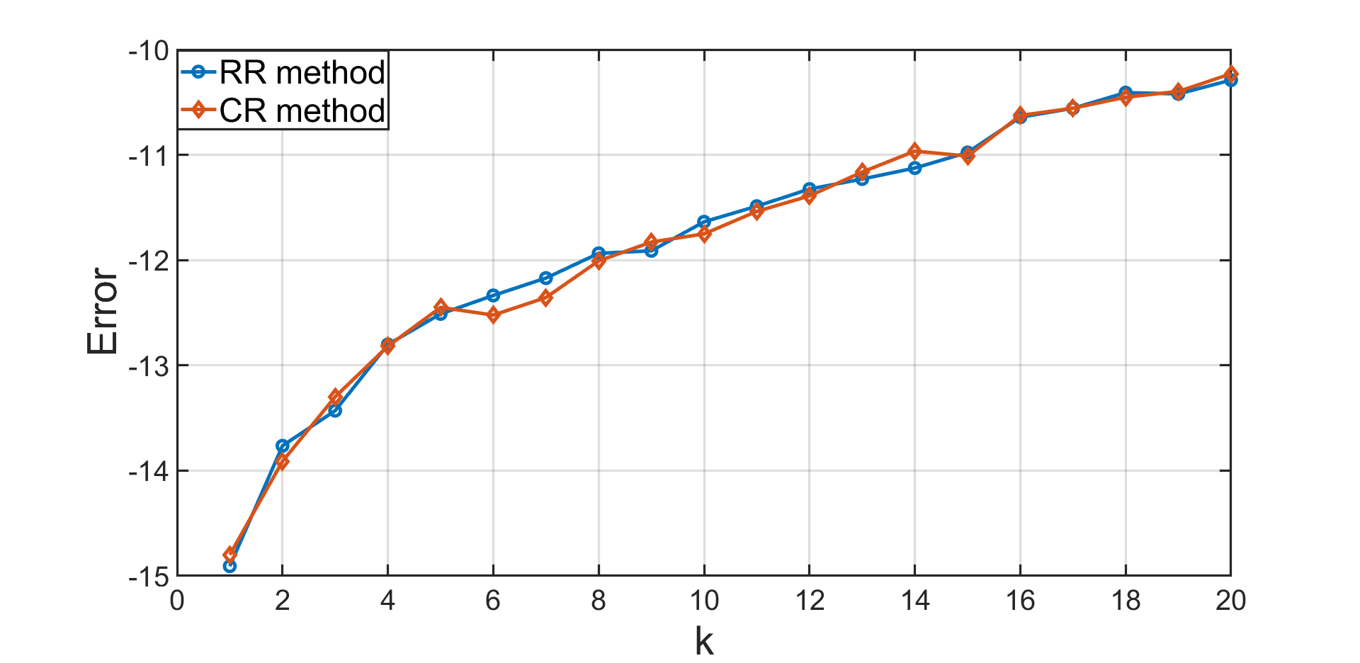
Figure 2 presents a comparison between and , which is obtained by taking different value of . Notably, the errors obtained from both methods are nearly identical and consistently remains less than . This demonstrates that the RR method is as effective as the CR method in determining Hermitian solutions for RBME (1).

Figure 3 depicts a comparison of the CPU time taken by the RR method and the CR method in finding the Hermitian solution of RBME (1). This comparison is conducted for various values of . Notably, the CPU time consumed by RR method is less compared to the CR method. This highlights the enhanced efficiency and time-saving nature of our proposed RR method compared to the CR method.
Next, we illustrate two examples for solving PDIEP for a Hermitian matrix.
Example 5.3.
To establish test data, we first generate a Hermitian matrix and compute its eigenpairs. Let , , and . Define .
Reconstruction from three eigenpairs : Let the prescribed partial eigeninformation be given by , , and , where , , and . Let
Construct the Hermitian matrix such that for . Let and . By using the transformations , we find the Hermitian solution to the matrix equation . We obtain
Then, is the desired Hermitian matrix. We have , , and . Errors , , and are in the order of and are negligible. Clearly, for .
Example 5.4.
To establish test data, we first generate a Hermitian matrix . Let
Let denote its eigenpairs. We have and , where
and their corresponding eigenvectors
Case . Reconstruction from one eigenpair : Let the prescribed partial eigeninformation be given by
Construct the Hermitian matrix such that for . By using the transformations , we find the Hermitian solution to the matrix equation . We obtain
Then, is the desired Hermitian matrix.
Case . Reconstruction from two eigenpairs : Let the prescribed partial eigeninformation be given by
Construct the Hermitian matrix such that for . By using the transformations , we find the Hermitian solution to the matrix equation . We obtain
Then, is the desired Hermitian matrix.
Case . Reconstruction from three eigenpairs : Let the prescribed partial eigeninformation be given by
Construct the Hermitian matrix such that for . By using the transformations , we find the Hermitian solution to the matrix equation . We obtain
Then, is the desired Hermitian matrix.
| Case | Case | Case | |||
|---|---|---|---|---|---|
| Eigenpair | Eigenpairs | Eigenpairs | |||
6 Conclusion
We have introduced an efficient method to obtain the least squares Hermitian solutions of the reduced biquaternion matrix equation . Our method involved transforming the constrained reduced biquaternion least squares problem into an equivalent unconstrained least squares problem of a real matrix system. This was achieved by utilizing the real representation matrix of the reduced biquaternion matrix and leveraging its specific structure. Additionally, we have determined the necessary and sufficient conditions for the existence and uniqueness of the Hermitian solution, along with a general form of the solution. These conditions and the general form of the solution were previously derived by Yuan et al. using the complex representation of reduced biquaternion matrices. In comparison, our approach exclusively involved real matrices and utilized real arithmetic operations, resulting in enhanced efficiency. We have also used our developed method to solve partially described inverse eigenvalue problems over the complex field. Finally, we have provided numerical examples to demonstrate the effectiveness of our method and its superiority over the existing method.
References
- [1] Moody Chu and Gene Golub. Inverse eigenvalue problems: theory, algorithms, and applications. OUP Oxford, 2005.
- [2] Biswa Datta. Numerical methods for linear control systems, volume 1. Academic Press, 2004.
- [3] Jie Ding, Yanjun Liu, and Feng Ding. Iterative solutions to matrix equations of the form . Comput. Math. Appl., 59(11):3500–3507, 2010.
- [4] Shan Gai. Theory of reduced biquaternion sparse representation and its applications. Expert Systems with Applications, 213:119–245, 2023.
- [5] Feliks Rouminovich Gantmacher and Joel Lee Brenner. Applications of the Theory of Matrices. Courier Corporation, 2005.
- [6] Gene H Golub and Charles F Van Loan. Matrix computations. JHU press, 2013.
- [7] Dai Hua and Peter Lancaster. Linear matrix equations from an inverse problem of vibration theory. Linear Algebra Appl., 246:31–47, 1996.
- [8] Tongsong Jiang and Musheng Wei. On solutions of the matrix equations and . Linear Algebra Appl., 367:225–233, 2003.
- [9] Peter Lancaster. Explicit solutions of linear matrix equations. SIAM Rev., 12:544–566, 1970.
- [10] An-Ping Liao and Yuan Lei. Least-squares solution with the minimum-norm for the matrix equation . Comput. Math. Appl., 50(3-4):539–549, 2005.
- [11] Sujit Kumar Mitra. Common solutions to a pair of linear matrix equations and . Proc. Cambridge Philos. Soc., 74:213–216, 1973.
- [12] A. Navarra, P. L. Odell, and D. M. Young. A representation of the general common solution to the matrix equations and with applications. Comput. Math. Appl., 41(7-8):929–935, 2001.
- [13] Soo-Chang Pei, Ja-Han Chang, and Jian-Jiun Ding. Commutative reduced biquaternions and their Fourier transform for signal and image processing applications. IEEE Trans. Signal Process., 52(7):2012–2031, 2004.
- [14] Soo-Chang Pei, Ja-Han Chang, Jian-Jiun Ding, and Ming-Yang Chen. Eigenvalues and singular value decompositions of reduced biquaternion matrices. IEEE Trans. Circuits Syst. I. Regul. Pap., 55(9):2673–2685, 2008.
- [15] Sang-Yeun Shim and Yu Chen. Least squares solution of matrix equation . SIAM J. Matrix Anal. Appl., 24(3):802–808, 2003.
- [16] Peng Wang, Shifang Yuan, and Xiangyun Xie. Least-squares Hermitian problem of complex matrix equation . J. Inequal. Appl., pages 1–13, 2016.
- [17] Guiping Xu, Musheng Wei, and Daosheng Zheng. On solutions of matrix equation . Linear Algebra Appl., 279(1-3):93–109, 1998.
- [18] Shi-Fang Yuan, Yong Tian, and Ming-Zhao Li. On Hermitian solutions of the reduced biquaternion matrix equation . Linear Multilinear Algebra, 68(7):1355–1373, 2020.
- [19] Shi-Fang Yuan and Qing-Wen Wang. L-structured quaternion matrices and quaternion linear matrix equations. Linear Multilinear Algebra, 64(2):321–339, 2016.
- [20] Fengxia Zhang, Weisheng Mu, Ying Li, and Jianli Zhao. Special least squares solutions of the quaternion matrix equation . Comput. Math. Appl., 72(5):1426–1435, 2016.
- [21] Fengxia Zhang, Musheng Wei, Ying Li, and Jianli Zhao. Special least squares solutions of the quaternion matrix equation with applications. Appl. Math. Comput., 270:425–433, 2015.
- [22] Fengxia Zhang, Musheng Wei, Ying Li, and Jianli Zhao. An efficient method for special least squares solution of the complex matrix equation . Comput. Math. Appl., 76(8):2001–2010, 2018.
- [23] Fengxia Zhang, Musheng Wei, Ying Li, and Jianli Zhao. The minimal norm least squares Hermitian solution of the complex matrix equation . J. Franklin Inst., 355(3):1296–1310, 2018.
- [24] Fengxia Zhang, Musheng Wei, Ying Li, and Jianli Zhao. An efficient method for least-squares problem of the quaternion matrix equation . Linear Multilinear Algebra, 70(13):2569–2581, 2022.