![[Uncaptioned image]](https://cdn.awesomepapers.org/papers/979f6f40-28ae-4028-89ea-77cb09714e68/x1.png)
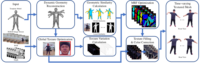
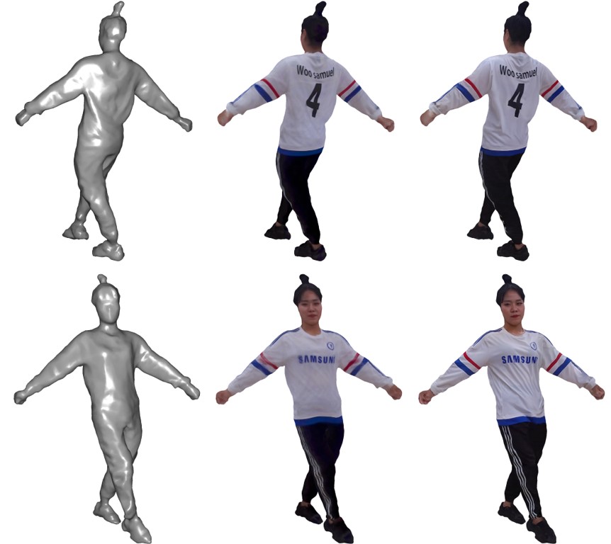
Our approach reconstructs a time-varying (spatiotemporal) texture map for a dynamic object using partial observations obtained by a single RGB-D camera. The frontal and rear views (top and bottom rows) of the geometry at two frames are shown in the middle left. Compared to the global texture atlas-based approach [KKPL19], our method produces more appealing appearance changes of the object. Please see the supplementary video for better visualization of time-varying textures.
Spatiotemporal Texture Reconstruction for Dynamic Objects
Using a Single RGB-D Camera
Abstract
This paper presents an effective method for generating a spatiotemporal (time-varying) texture map for a dynamic object using a single RGB-D camera. The input of our framework is a 3D template model and an RGB-D image sequence. Since there are invisible areas of the object at a frame in a single-camera setup, textures of such areas need to be borrowed from other frames. We formulate the problem as an MRF optimization and define cost functions to reconstruct a plausible spatiotemporal texture for a dynamic object. Experimental results demonstrate that our spatiotemporal textures can reproduce the active appearances of captured objects better than approaches using a single texture map. {CCSXML} <ccs2012> <concept> <concept_id>10010147.10010371.10010382.10010384</concept_id> <concept_desc>Computing methodologies Texturing</concept_desc> <concept_significance>500</concept_significance> </concept> </ccs2012>
\ccsdesc[500]Computing methodologies Texturing \printccsdesc
1 Introduction
3D reconstruction methods using RGB-D images have been developed for static scenes [NIH∗11, NZIS13, DNZ∗17] and dynamic objects [NFS15, IZN∗16, DKD∗16]. The appearance of the reconstructed 3D models, which are often represented as color meshes, is crucial in realistic content creation for Augmented Reality (AR) and Virtual Reality (VR) applications. Subsequent works have been proposed to improve the color quality of reconstructed static scenes [GWO∗10, ZK14, JJKL16, FYY∗18, LGY19] and dynamic objects [OERF∗16, DCC∗18, GLD∗19]. For static scenes, most of the approaches generate a global texture atlas [WMG14, JJKL16, FYY∗18, LGY19], and the main tasks consist of two parts: selecting the best texture patches from input color images and relieving visual artifacts such as texture misalignments and illumination differences when the selected texture patches are combined.
While single texture map is widely used to represent a static scene, it is not preferred for a dynamic object due to appearance changes over time. A multi-camera system could facilitate creating a spatiotemporal (time-varying) texture map of a dynamic object, but such setup may not be affordable for ordinary users. As an alternative, recovering a spatiotemporal texture using a single RGB-D camera can be a practical solution.
Previous reconstruction methods using a single RGB-D camera maintain and update voxel colors in the canonical frame [NFS15, IZN∗16, GXY∗17, YGX∗17, YZG∗18]. However, this voxel color based approach cannot properly represent detailed time-varying appearances, e.g., cloth wrinkles and facial expression changes for capturing humans. Kim et al. [KKPL19] proposed a multi-scale optimization method to reconstruct a global texture map of a dynamic model under a single RGB-D camera setup. Still, the global texture map is static and cannot represent time-varying appearances of a dynamic object.
In this work, we propose a novel framework to generate a spatiotemporal texture map for a dynamic template model using a single RGB-D camera. Given a template model that is dynamically aligned with input RGB-D images, our main objective is to produce a spatiotemporal texture map that provides a time-varying texture of the model. Since a single camera can obtain only partial observations at each frame, we bring color information from other frames to complete a spatiotemporal texture map. We formulate a Markov random field (MRF) energy, where each node in the MRF indicates a triangular face of the dynamic template model at a frame. By minimizing the energy, for every frame, an optimal image frame to be used for texture mapping each face can be determined. Recovering high-quality textures is another goal of this work because it is crucial for free-viewpoint video generation of a dynamic model. Due to imperfect motion tracking, texture drifts may happen when input color images are mapped onto the dynamic template model. To resolve the problem, we find optimal texture coordinates for the template model on all input color frames. As a result, our framework can handle time-varying appearances of dynamic objects better than the previous approach [KKPL19] based on a single static texture map.
The key contributions are summarized as follows:
-
•
A novel framework to generate a stream of texture maps for a dynamic template model from color images captured by a single RGB-D camera.
-
•
An effective MRF formulation including selective weighting to compose high-quality time-varying texture maps from single view observations.
-
•
An accelerated approach to optimize texture coordinates for resolving texture drifts on a dynamic template model.
-
•
Quantitative evaluation and user study to measure the quality of reconstructed time-varying texture maps.
 |
2 Related Work
2.1 Dynamic Object Reconstruction
3D reconstruction systems for dynamic objects can be classified into two categories: template-based and templateless. A representative templateless work is DynamicFusion [NFS15], which shows real-time non-rigid reconstruction using a single depth camera. VolumeDeform [IZN∗16] considers a correspondence term made from SIFT feature matching to improve motion tracking. BodyFusion [YGX∗17], which specializes in human body, exploits human skeleton information for surface tracking and fusion.
Template-based non-rigid reconstruction assumes that a template model for the target object is given, and deforms the template model to be aligned with input data. Most template-based methods [LAGP09, ZNI∗14, GXW∗15, GXW∗18] are based on embedded deformation (ED) graph model [SSP07], which is also utilized in templateless works [LVG∗13, DTF∗15, DKD∗16, DDF∗17]. High-end reconstruction systems using a number of cameras can capture a complete mesh of the target object at each timestamp, so they commonly use template tracking between keyframes for compressing redundant data [CCS∗15, PKC∗17, GLD∗19].
2.2 Appearances of Reconstructed Models
Static scenes
When scanning a static scene with a single RGB-D camera, color information obtained by volumetric fusion tends to be blurry due to inaccurate camera pose estimation. Gal et al. [GWO∗10] optimize projective mapping from each face of a mesh onto one of the color images by performing combinatorial optimization on image labels and adjusting 2D coordinates of projected triangles. Zhou and Koltun [ZK14] jointly optimize camera poses, non-rigid correction functions, and vertex colors to increase the photometric consistency. Jeon et al. [JJKL16] optimize texture coordinates projected on input color images to resolve misalignments of textures. Bi et al. [BKR17] propose patch-based optimization to align images against large misalignments between frames. Fu et al. [FYY∗18] and Li et al.[LGY19] improve the color of a reconstructed mesh by finding an optimal image label for each face. Fu et al. [FYLX20] jointly optimize texture and geometry for better correction of textures. Huang et al. [HTD∗20] exploit a deep learning approach to reconstruct realistic textures.
Non-rigid objects with multiple cameras
Non-rigid object reconstruction has received attention in the context of performance capture using multi-view camera setup [CCS∗15, PKC∗17, DKD∗16, OERF∗16]. Fusion4D [DKD∗16] is a real-time performance capture system using multiple cameras, and it shows the capability to reconstruct challenging non-rigid scenes. However, it uses volumetrically fused vertex colors to represent the appearance, resulting in blurred colors of the reconstructed model. To resolve the problem, Holoportation [OERF∗16] proposes several heuristics, including color majority voting. Montage4D [DCC∗18] considers misregistration and occlusion seams to obtain smooth texture weight fields. Offline multi-view performance capture systems[CCS∗15, GLD∗19] generate a high-quality texture atlas at each timestamp using mesh parameterization, and temporally coherent atlas parameterization [PKC∗17] was proposed to increase the compression ratio of a time-varying texture map.
Non-rigid scenes with a single camera
Kim et al. [KKPL19] produces a global texture map for a dynamic object by optimizing texture coordinates on the input color images in a single RGB-D camera setup. Pandey et al. [PTY∗19] propose semi-parametric learning to synthesize images from arbitrary novel viewpoints. PIFu [SHN∗19] combines learning-based 3D reconstruction, volumetric deformation, and light-weight bundle adjustment to reconstruct a clothed human model in a few seconds from a single RGB-D stream. These methods produce either a single texture map for the reconstructed dynamic model [KKPL19, SHN∗19] or temporally independent blurry color images for novel viewpoints [PTY∗19]. They all cannot generate a sequence of textures varying with motions of the reconstructed model over time. Our framework aims to produce a visually plausible spatiotemporal texture for a dynamic object with a single RGB-D camera.
3 Problem Definition
3.1 Spatiotemporal Texture Volume
Given a triangular mesh of the template model, we assume that a non-rigid deformation function is given for each time frame , satisfying , where denotes the deformed template mesh fitted to the depth map . Our goal is to produce a spatiotemporal (time-varying) texture map for the dynamic template mesh. By embedding onto a 2D plane using a parameterization method [Mic11], each triangle face of is mapped onto a triangle in the 2D texture domain. A spatiotemporal texture map can be represented as stacked texture maps (or spatiotemporal texture volume), whose size is , where is the side length of a rectangular texture map and is the number of input frames. We assume that our mesh keeps a fixed topology in the deformation sequence, and the position of face in the 2D texture domain remains the same regardless of time . Only the texture information of face changes with time to depict dynamically varying object appearances.
3.2 Objectives
To determine the texture information for face of the deformed mesh at time in a texture volume, we need to solve two problems: color image selection and texture coordinate determination. We should first determine which color image in the input will be used for extracting the texture information. A viable option is to use the color image at time . However, depending on the camera motion, face may not be visible in , and in that case, texture should be borrowed from another color image where the face is visible. Moreover, when there are multiple such images, the quality of input images should be considered, as some images can provide sharper textures than others.
Once we have selected the color image , we need to determine the mapped position of in . Since we already have the deformed mesh at time , the mapping of onto can be obtained by projecting face in onto . However, due to the errors in camera tracking and non-rigid registration, mappings of onto different input color images may not be completely aligned. If we use such mappings for texture sampling, the temporal texture volume would contain little jitters in the part corresponding to .
An overall pipeline of our system is shown in Figure 1. Starting from RGB-D images and a deforming model, we determine the aligned texture coordinates using global texture optimization (Section 4). Then, to select color images for each face at all timestamps, we utilize MRF optimization (Section 5). To reduce redundant calculation, we pre-compute and tabulate the measurements that are required to construct the cost function before MRF optimization. Finally, we build a spatiotemporal texture volume and refine textures by conducting post-processing.
4 Spatiotemporal Texture Coordinate Optimization
Camera tracking and calibration errors induce misalignments among textures taken from different frames. Non-rigid registration errors incur additional misalignments in the case of dynamic objects. Kim et al. [KKPL19] proposed an efficient framework for resolving texture misalignments for a dynamic object. For a template mesh , the framework optimizes the texture coordinates of mesh vertices on the input color images so that sub-textures of each face extracted from different frames match each other. The optimization energy is defined to calculate the photometric inconsistency among textures taken from different frames:
| (1) |
where denotes proxy colors computed by averaging . and are solved using alternating optimization, where is initialized with the projected positions of the vertices of deformed meshes on corresponding color images.
To obtain texture coordinates with aligned textures among frames, we adopt the framework of Kim et al. [KKPL19] with some modification. Their approach selects keyframes to avoid using blurry color images (due to abrupt motions) in the image sequence and considers only those keyframes in the optimization. In contrast, we need to build a spatiotemporal texture volume that contains every timestamp, so optimization should involve all frames. We modify the framework to reduce computational overhead while preserving the alignment quality.
Our key observation is that the displacements of texture coordinates determined by the optimization process smoothly change among adjacent frames. In Figure 2, red dots indicate initially projected texture coordinates of vertices , and the opposite endpoints of blue lines indicate optimized texture coordinates . Based on the observation, we regularly sample the original input frames and use the sampled frames for texture coordinate optimization. Texture coordinates of the non-sampled frames are determined by linear interpolation of the displacements at the sampled frames.
In the optimization process, we need to compute the proxy colors from the sampled color images. To avoid invalid textures (e.g., background colors), we segment foreground and background on the images using depth information with GrabCut [RKB04], and give small weights for background colors. After optimization with sampled images and linear interpolation for non-sampled images, most of the texture misalignments are resolved. Then, we perform a few iterations of texture coordinate optimization involving all frames for even tighter alignments.
Our modified framework is about five times faster than the original one [KKPL19]. In our experiment, where we sampled every four images from 265 frames and the template mesh consists of 20k triangles, the original and our frameworks took 50 and 11 minutes, respectively.
 |
 |
 |
| (a) | (b) | (c) |
5 Spatiotemporal Texture Volume Generation
After texture coordinate determination, we have aligned texture coordinates on every input image for each face of the dynamic template mesh. The remaining problem is to select the color image for every face at each time frame . To this end, we formulate a labeling problem.
Let be the candidate set of image frames for a face , where consists of image frames in which face is visible. Our goal is to determine the label from for each face at each time . If we have a quality measure for input color images, a direct way would be to select the best quality image in for all . However, this approach produces a static texture map that does not reflect dynamic appearance changes.
To solve the labeling problem, we use MRF (Markov Random Field) [GG84, Bes86] optimization. The label for face at time is a node in the MRF graph, and there are two kinds of edges in the graph. A spatial edge connects two nodes and if faces and are adjacent to each other in the template mesh. A temporal edge connects two nodes and in the temporal domain. To determine the value of on the MRF graph, we minimize the following cost function.
5.1 Cost Function
Our cost function consists of data term and smoothness term as follows,
| (2) |
where is the set of faces in the template mesh and is the set of adjacent nodes of in the MRF graph.
5.1.1 Data Term
In many cases, a natural choice for the label of would be frame . However, if face is not visible in , i.e., , we cannot choose for . In addition, even in the case that , could be blurry and some other , , could be a better choice. To find a plausible label for in either case, we assume that similar shapes would have similar textures too. The data term consists of two terms and :
| (3) |
is designed to avoid assigning low-quality texture, such as blurred region. is defined as follows:
| (4) |
where is a step function whose value is 1 if , and 0 otherwise. The first term estimates the blurriness of face by measuring the changes of the optimized texture coordinates of vertices among consecutive frames, and . The second term uses the dot product of the face normal and the camera’s viewing direction . prefers to assign an image label if it provides sharp texture and avoids texture distortion due to slanted camera angle. By taking a step function in , no penalty is imposed once the image quality is above the threshold, keeping the plausible label candidates as much as possible.
ensures to select a timestamp with a similar shape. The geometry term measures global similarity and local similarity between shapes:
| (5) |
considers overall geometric similarity between frames and is defined as follows:
| (6) |
where denotes an image pixel, and is the clipped difference between two depth values and that are rendered from and , respectively. Here, denotes a 6-DoF rigid transformation that aligns to .
is devised to find an image label such that the deformed template meshes and are geometrically similar. It measures the sum of depth differences over the union area of the projected meshes on image , , where in Eq. (6) is a pixel in the union area on . We obtain with RANSAC based rigid pose estimation that utilizes coordinate pairs of the same vertices in and .
Even though we found a geometrically similar frame with , local shapes around face do not necessarily match among and . Local similarity guides shape search using local geometric information and is defined as , where denotes one of three vertex pairs from face in and . We utilize SHOT [TSDS10] to obtain a descriptor of the local geometry calculated for each vertex. SHOT originally uses the Euclidean distance to find the neighborhood set. Since we have a template mesh, we exploit the geodesic distance to obtain the local surface feature. To reduce the effect of noise, we apply median filter to SHOT descriptor values of vertices.
5.1.2 Smoothness Term
The smoothness term is defined for each edge of the MRF graph. Its role is to reduce seams in the final texture map and to control texture changes over time. To this end, we define spatial smoothness in texture map domain and temporal smoothness over time axis of the spatiotemporal texture volume. That is,
| (7) |
is defined as follows:
| (8) |
where is a shared edge between two faces and , and are the corresponding image pixels when the edge is mapped onto and . If the nodes and have different image labels, color information should match along the shared edge to prevent a seam in the final texture map. In addition, we use the differences of gradient images, and , to match the color changes around the edge between and .
is defined as follows:
| (9) |
where denotes the projection of face onto and , and denotes corresponding image pixels on the projected faces. measures the intensity differences and promotes soft transition of the texture assigned to over time shift .
 |
 |
 |
| (a) | (b) | (c) |
 |
| (d) Average SSIM values in colored boxes of (c) |
5.2 Selective Weighting for Dynamic Textures
Textures on a dynamic object may have different dynamism depending on their positions. Some parts can have dynamic appearance changes with object motions, e.g., cloth wrinkles under human motions, while other parts may have almost no changes of textures over time, e.g., naked forearms of the human body. We verified this property with an experiment. After we have obtained optimized texture coordinates for a deforming mesh sequence, we can build an initial incomplete spatiotemporal texture volume by simply copying the visible parts in the input images onto the corresponding texture maps (Figure 3a). Then, we compute the SSIM map between adjacent frames in the texture volume on the overlapping areas (Figure 3b). Figure 3d shows changes in the SSIM values over time for the marked parts in Figure 3c. In the blue and cyan colored regions, SSIM fluctuates along time, meaning that these parts have versatile textures. Such parts need to be guaranteed for dynamism in the final spatiotemporal texture, while smooth texture changes would be fine for other parts.
To reflect this property in the MRF optimization, we modify the smoothness terms on MRF edges. We ignore a temporal MRF edge if the labels of the linked nodes exhibit a lower SSIM value, i.e., less correlation. In our temporal selective weighting scheme, the following new temporal smoothness term replaces in Eq. (7):
| (10) |
where is the average SSIM value of the pixels inside face computed among consecutive frames. is a step function whose value is 1 if , and 0 otherwise. This scheme encourages the dynamism of textures over time when there is less correlation among frames.
In a similar way, we update the spatial smoothness term in Eq. (7) as follows:
| (11) |
where . If there is a label with a small SSIM value in , the part has a risk of temporal discontinuity due to the updated temporal smoothness term in Eq. (10). Therefore, in that case, we enforce the spatial smoothness term to impose spatial coherence when temporal discontinuity happens. In Figure 3c, the red box is likely to exhibit temporal changes, e.g., mouth opening. Our spatial selective weighting scheme increases the spatial smoothness term for the red box to secure spatially coherent changes of texture.
5.3 Labeling and Post Processing
Since our MRF graph is large to solve, we divide the problem and solve it using alternating optimization. The idea of fixing a subset and optimizing the others is known as block coordinate descent (BCD). In [CK14, TWW∗16], the BCD technique is applied to uniform and non-uniform MRF topology. Our MRF graph consists of spatial edges connecting adjacent mesh faces at a single frame and temporal edges connecting corresponding mesh faces at consecutive frames. As a result, our MRF topology is spatially non-uniform but temporally uniform. We subdivide the frames into two sets: even-numbered and odd-numbered. We first conduct optimization for even-numbered frames without temporal smoothness terms. After that, we optimize for odd-numbered frames while fixing the labels of even-numbered frames, where temporal smoothness terms become unary terms. We iterate alternating optimization among even- and odd-numbered frames until convergence. To optimize a single set MRF graph (even or odd), we use an open-source library released by Daniel et al. [TWW∗16].
 |
 |
 |
| (a) | (b) | (c) |
After labeling is done, we have a frame label per face at each timestamp. Then we fill the spatiotemporal texture atlas volume by copying texture patches from the labeled frames. When there are drastic brightness changes among different frames, spatial seams may happen on label boundaries (Figure 4a). To handle such cases, we apply gradient processing [PKCH18] to texture slices in the volume, resolving spatial seams (Figure 4c).
|
 |
 |
||
|
 |
 |
||
|
 |
 |
||
| (a) mouth changes | (b) wrinkle changes |
 |
 |
| (a) | (b) |
6 Results
6.1 Experiment Details
Setup
All datasets shown in this paper were recorded by an Azure Kinect DK [Mic20] with 3072p resolution for color images, and for depth images. All experiments were conducted on a workstation equipped with an Intel i7-7700K 4.2GHz CPU, 64GB RAM, and NVIDIA Titan RTX GPU. Our RGB-D sequences used for experiments contain 200 to 500 frames. The size of a texture slice in a spatiotemporal texture volume is . We set , , , , , for all examples. Source code for our method can be found at https://github.com/posgraph/coupe.Sptiotemporal-Texture/.
| Scene | 1 | 2 | 3 | 4 | 5 | 6 |
| # Frame | 265 | 210 | 372 | 247 | 484 | 210 |
| Tex Opt (min) | 11.0 | 9.3 | 8.8 | 5.6 | 19.2 | 8.6 |
| Labeling (min) | 23.0 | 17.9 | 20.0 | 23.9 | 56.0 | 25.1 |
Timing
The global texture coordinate optimization takes about minutes for a dynamic object. Solving MRF on average takes about seconds per frame. The color correction takes about 20 seconds per frame, but this step can be parallelized. Timing details are shown in Table 1.
Dynamic object reconstruction
We reconstruct a template model by rotating a color camera around the motionless object and using Agisoft Metashape111https://www.agisoft.com/ for 3D reconstruction. Then we apply mesh simplification [HCC06] to the reconstructed template model and reduce the number of triangle faces to about 1030k. To obtain a deformation sequence of the template mesh that matches the input depth stream, we adopt a non-rigid registration scheme based on an embedded deformation (ED) graph [SSP07]. The scheme parameterizes a non-rigid deformation field using a set of 3D affine transforms. It estimates the deformation field to fit mesh into an input depth map at time using an motion regularizer [GXW∗15].
6.2 Analysis
Texture coordinate optimization
To accelerate the texture coordinate optimization process, we regularly sample frames and interpolate the texture coordinate displacements computed from the samples. Table 2 shows that our approach achieves almost the same accuracy compared to the original one using all frames. Using fewer sample frames reduces more computation, and we sample every four frames for the time-accuracy tradeoff.
| sampling | 1/2 | 1/3 | 1/4 | 1/5 |
| error ratio | 1.0063 | 1.02220 | 1.02309 | 1.0427 |
Global & local geometric similarity
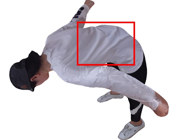
Our method utilizes global and local geometric similarities to assign the most reasonable frame labels to the faces of the dynamic template mesh. In Figure 6a, back parts that do not show obvious geometric patterns are not distinguishable by local similarity, and global similarity helps to assign proper frame labels. On the other hand, as shown in Figure 6b, local similarity helps to find appropriate textures if local geometry changes should be considered to borrow natural appearances from other frames.
 |
 |
| (a) | (b) |
| Metrics | Methods | Scene 1 | Scene2 | Scene 3 | Scene 4 | Scene 5 | Scene 6 |
| PSNR (every frame) | Kim et al. [KKPL19] | 28.1677 | 29.3667 | 26.5816 | 27.1487 | 21.8453 | 27.2445 |
| Ours | 28.6900 | 30.6023 | 28.9535 | 28.0716 | 23.4724 | 27.3731 | |
| PSNR (unseen frame (1/6)) | Kim et al. [KKPL19] | 28.1243 | 29.2732 | 26.6415 | 27.1501 | 21.6907 | 26.8947 |
| Ours (1/3) | 28.8495 | 29.9831 | 28.4498 | 27.6200 | 23.1869 | 27.2290 | |
| Ours (1/2) | 28.8797 | 30.0269 | 28.5851 | 27.8092 | 23.2763 | 27.2566 | |
| Blurriness (Crete et al. [CDLN07]) | Input images | 0.7937 | 0.8004 | 0.8906 | 0.9095 | 0.8220 | 0.8440 |
| Kim et al. [KKPL19] | 0.7971 | 0.8006 | 0.8865 | 0.9101 | 0.8384 | 0.8514 | |
| Ours | 0.7896 | 0.7912 | 0.8824 | 0.9065 | 0.8104 | 0.8425 |
 |
 |
 |
| (a) | (b) frame 26 | (c) frame 34 |
Selective weighting
Figure 7 shows that spatial selective weighting can help preventing abnormal seams. Figure 5 compares different temporal weighting schemes. Our temporal selective weighting makes the mouth motion consistent (Figure 5a), and incurs more dynamism on the back part by dropping the smoothness constraint (Figure 5b).
6.3 Quantitative Evaluation
Coverage
We computed the amount of textures generated by our method. Naive projection can cover 29.5% 39.6% of the mesh faces depending on the scene, while our reconstructed textures always cover the entire surfaces.
Reconstruction error
We quantitatively measured the reconstruction errors by calculating PSNR between input images and rendered images of the reconstructed textures. To circumvent slight misalignments, we subdivided the images into small grid patches and translated the patches to find the lowest MSE. The top rows of Table 3 show that our spatiotemporal textures reconstruct the input textures more accurately than global textures [KKPL19]. Even when intentionally we did not use some input images (e.g., every even frames) for texture reconstruction, our method could successfully produce dynamic textures, as shown in the middle rows of Table 3.
Texture quality
We quantitatively assessed the quality of reconstructed textures using a blur metric [CDLN07]. The bottom rows of Table 3 show our results are sharper than global textures [KKPL19]. Our results are even sharper than the input images on average, as texture patches containing severe motion blurs are avoided in our MRF optimization. See Figure 8 for illustration.
6.4 Qualitative Comparison
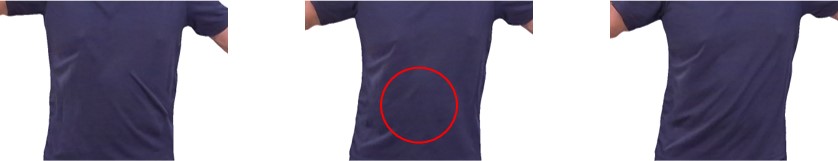
In Figure 13a, we compare our results with a texture-mapped model using single images. The single image-based texture has black regions since some parts are invisible at a single frame, while our texture map covers the whole surface of the object. Compared to global texture map [KKPL19], our spatiotemporal texture is more appropriate to convey temporal contents (Figure 13b). In particular, wrinkles on the clothes are expressed better. Additional results are shown in Figures 14 and 15.
6.5 User Study
For a spatiotemporal texture reconstructed using our method, texture quality of originally visible regions can be measured by comparing with the corresponding regions in the input images, as we did in Section 6.3. However, for regions invisible in the input images, there are no clear ground truths. Even if an additional camera is set up to capture those invisible regions, the captured textures are not necessarily the only solutions, as various textures can be applied to a single shape, e.g., eyes may be open or closed with the same head posture.
To evaluate the quality of reconstructed textures for originally invisible regions without ground truths, we conducted a user study using Amazon Mechanical Turk (AMT). We generated a set of triple images using input images, dynamic model rendered with spatiotemporal texture, and dynamic model rendered with global texture [KKPL19]. We picked the triple images to be as similar as possible to each other, while removing the backgrounds of input images. Figure 9a shows an example. We prepared 40 image triples (120 images) and asked to evaluate whether the given images are realistic or not in two ways: One task is to choose a more realistic image among a pair of images. The other is to score how realistic a given single image is on a scale of 1-10. We set 25 workers whose hit approval rates are over 98% to answer a single question. As a result, we collected total 3,000 pairwise comparison results and 3,000 scoring results.
The preference matrix in Table 4 summarizing the pairwise comparison results shows that the input images are clearly preferred to rendered images using reconstructed textures. This result would be inevitable as geometric reconstruction errors have introduced unnaturalness on top of texture reconstruction artifacts. The errors are mainly caused by the template deformation method, which may not completely reconstruct geometric details. For example, in Figure 9a, the sleeve of T-shirt is tightly attached to the arm in the reconstructed mesh. Still, Table 4 shows our spatiotemporal textures dominate global textures, where only texture reconstruction qualities are compared. The scoring results summarized in Figure 9b show similar conclusions.
 |
 |
| (a) sample image triple | (b) scoring result summary |
| Raw image | [KKPL19] | Ours | |
| Raw image | - | 863 | 718 |
| [KKPL19] | 137 | - | 190 |
| Ours | 182 | 810 | - |
 |
 |
 |
| (a) Target frame | (b) PIFu [SHN∗19] | (c) Ours |
6.6 Comparison with Learning-based Methods
As mentioned in Section 2, there are learning-based methods to reconstruct textures of objects. However, there are important differences between our method and those methods. Firstly, our method uses a template mesh and an image sequence from a single camera as the input, whereas the learning-based methods use a single image [SHN∗19, PTY∗19] or multi-view images [SHN∗19]. Although it is unfair, we tested the authors’ implementation of [SHN∗19] on single images of our dataset (Figure 10). The generated textures on the originally invisible areas are clearly worse than our results. Note that multi-view images that can be used in [SHN∗19] should be captured by multiple cameras at the same time. Then the setting differs from our case of a single camera, making comparison using multi-view images inappropriate. Secondly, due to memory limitation, the networks of [SHN∗19, PTY∗19] cannot fully utilize the textures of our 4K dataset. This would lead to poor quality compared to our results. Thirdly, the learning-based methods target only humans, while our method does not have the limitation, as demonstrated in the top two examples of Figure 14. Finally, our method reconstructs a completed texture volume that can be readily used for generating consistent novel views in a traditional rendering pipeline, but synthesized novel views from learning-based methods are not guaranteed to be consistent.
 |
 |
 |
 |
| (a) frame 50 | (b) frame 60 | (c) frame 70 | (d) frame 80 |
 |
| (e) input images and reconstructed textures on frames 160-162. |
6.7 Discussions and Limitations
Rich textures
Our method would work for rich textures as far as our texture coordinate optimization works properly. Texture coordinate optimization may fail in an extreme case. For example, when the texture is densely repeated, the misalignment in geometric reconstruction could be larger than the texture repetition period. Then, the texture correspondence among different frames could be wrongly optimized.
Computation time
Our approach takes quite some time and it would be hard to become real-time. On the other hand, texture reconstruction for a model is needed to be done only once, and our method produces high-quality results that can be readily used in a conventional rendering pipeline.
Dependency on geometry processing
If non-rigid registration of dynamic geometry fails completely, our texture reconstruction fails accordingly. However, the main focus of this paper is to reconstruct high-quality textures, and our method would be benefited from the advances of single-view non-rigid registration techniques. In our approach, texture coordinate optimization helps handle possible misalignments from non-rigid registration of various motions. For fast motions, as shown in Figure 8, our labeling data term could filter out blurry textures, replacing them with sharper ones.
Fixed topology
Variant lights and relighting
Our method may not produce plausible texture brightness changes in a variant lighting environment. In Figure 11, a directional light is continuously moving when the input images are captured. However, the reconstructed textures on invisible regions show sudden brightness changes at some frames. As a result, sometimes temporal flickering can be found on originally invisible regions. Another limitation of our method is that lighting is not separated from textures but included in the restored textures. This limitation would hinder relighting of the textured objects, but could be resolved by performing intrinsic decomposition on the input images.
Unseen textures
Our method cannot generate textures that are not contained in the input images. Unnatural textures could be produced for regions invisible at all frames (Figure 12).
7 Conclusions
We have presented a novel framework for generating a time-varying texture map (spatiotemporal texture) for a dynamic 3D model using a single RGB-D camera. Our approach adjusts the texture coordinates and selects an effective frame label for each face of the model. The proposed framework generates plausible textures conforming to shape changes of a dynamic model.
There are several ways to improve our approach. First, to conduct the labeling process more efficiently, considering a specific period like an approach by Liao [LJH13] would be a viable option. Second, our framework separates the 3D registration part and texture map generation part. We expect better results if the geometry and texture are optimized jointly [FYLX20].
Acknowledgements
This work was supported by the Ministry of Science and ICT, Korea, through IITP grant (IITP-2015-0-00174), NRF grant (NRF-2017M3C4A7066317), and Artificial Intelligence Graduate School Program (POSTECH, 2019-0-01906).
 |
 |
| (a) comparison with single-view reconstruction | (b) comparison with global texture map [KKPL19] |
 |
 |
 |
 |
 |
 |
 |
 |
 |
 |
References
- [Bes86] Besag J.: On the statistical analysis of dirty pictures. Journal of the Royal Statistical Society. Series B (Methodological) 48, 3 (1986), 259–302.
- [BKR17] Bi S., Kalantari N. K., Ramamoorthi R.: Patch-based optimization for image-based texture mapping. ACM TOG 36, 4 (2017), 106–1.
- [CCS∗15] Collet A., Chuang M., Sweeney P., Gillett D., Evseev D., Calabrese D., Hoppe H., Kirk A., Sullivan S.: High-quality streamable free-viewpoint video. ACM TOG 34, 4 (2015), 1–13.
- [CDLN07] Crete F., Dolmiere T., Ladret P., Nicolas M.: The blur effect: perception and estimation with a new no-reference perceptual blur metric. In Proc. SPIE (2007).
- [CK14] Chen Q., Koltun V.: Fast MRF optimization with application to depth reconstruction. In Proc. CVPR (2014).
- [DCC∗18] Du R., Chuang M., Chang W., Hoppe H., Varshney A.: Montage4D: Interactive seamless fusion of multiview video textures. In Proc. ACM SIGGRAPH Symposium on I3D (2018).
- [DDF∗17] Dou M., Davidson P., Fanello S. R., Khamis S., Kowdle A., Rhemann C., Tankovich V., Izadi S.: Motion2fusion: Real-time volumetric performance capture. ACM TOG 36, 6 (2017), 1–16.
- [DKD∗16] Dou M., Khamis S., Degtyarev Y., Davidson P., Fanello S. R., Kowdle A., Escolano S. O., Rhemann C., Kim D., Taylor J., Kohli P., Tankovich V., Izadi S.: Fusion4d: Real-time performance capture of challenging scenes. ACM TOG 35, 4 (2016), 1–13.
- [DNZ∗17] Dai A., Nießner M., Zollöfer M., Izadi S., Theobalt C.: Bundlefusion: Real-time globally consistent 3D reconstruction using on-the-fly surface re-integration. ACM TOG 36, 3 (2017), 1–18.
- [DTF∗15] Dou M., Taylor J., Fuchs H., Fitzgibbon A., Izadi S.: 3D scanning deformable objects with a single RGBD sensor. In Proc. CVPR (2015).
- [FYLX20] Fu Y., Yan Q., Liao J., Xiao C.: Joint texture and geometry optimization for rgb-d reconstruction. In Proc. CVPR (2020).
- [FYY∗18] Fu Y., Yan Q., Yang L., Liao J., Xiao C.: Texture mapping for 3D reconstruction with rgb-d sensor. In Proc. CVPR (2018).
- [GG84] Geman S., Geman D.: Stochastic relaxation, gibbs distributions, and the bayesian restoration of images. IEEE TPAMI, 6 (1984), 721–741.
- [GLD∗19] Guo K., Lincoln P., Davidson P., Busch J., Yu X., Whalen M., Harvey G., Orts-Escolano S., Pandey R., Dourgarian J., Tang D., Tkach A., Kowdle A., Cooper E., Dou M., Fanello S., Fyffe G., Rhemann C., Taylor J., Debevec P., Izadi S.: The relightables: Volumetric performance capture of humans with realistic relighting. ACM TOG 38, 6 (2019), 1–19.
- [GWO∗10] Gal R., Wexler Y., Ofek E., Hoppe H., Cohen-Or D.: Seamless montage for texturing models. Computer Graphics Forum 29, 2 (2010), 479–486.
- [GXW∗15] Guo K., Xu F., Wang Y., Liu Y., Dai Q.: Robust non-rigid motion tracking and surface reconstruction using L0 regularization. In Proc. ICCV (2015).
- [GXW∗18] Guo K., Xu F., Wang Y., Liu Y., Dai Q.: Robust non-rigid motion tracking and surface reconstruction using L0 regularization. IEEE TVCG 24, 5 (2018), 1770–1783.
- [GXY∗17] Guo K., Xu F., Yu T., Liu X., Dai Q., Liu Y.: Real-time geometry, albedo, and motion reconstruction using a single RGB-D camera. ACM TOG 36, 3 (2017), 1.
- [HCC06] Huang F.-C., Chen B.-Y., Chuang Y.-Y.: Progressive deforming meshes based on deformation oriented decimation and dynamic connectivity updating. In Symposium on Computer Animation (2006).
- [HTD∗20] Huang J., Thies J., Dai A., Kundu A., Jiang C., Guibas L. J., Nießner M., Funkhouser T.: Adversarial texture optimization from rgb-d scans. In Proc. CVPR (2020).
- [IZN∗16] Innmann M., Zollhöfer M., Nießner M., Theobalt C., Stamminger M.: Volumedeform: Real-time volumetric non-rigid reconstruction. In Proc. ECCV (2016).
- [JJKL16] Jeon J., Jung Y., Kim H., Lee S.: Texture map generation for 3D reconstructed scenes. The Visual Computer 32, 6-8 (2016), 955–965.
- [KKPL19] Kim J., Kim H., Park J., Lee S.: Global texture mapping for dynamic objects. In Computer Graphics Forum (2019), vol. 38, pp. 697–705.
- [LAGP09] Li H., Adams B., Guibas L. J., Pauly M.: Robust single-view geometry and motion reconstruction. In ACM SIGGRAPH Asia (2009).
- [LGY19] Li W., Gong H., Yang R.: Fast texture mapping adjustment via local/global optimization. IEEE TVCG 25, 6 (2019), 2296–2303.
- [LJH13] Liao Z., Joshi N., Hoppe H.: Automated video looping with progressive dynamism. ACM TOG 32, 4 (2013), 1–10.
- [LVG∗13] Li H., Vouga E., Gudym A., Luo L., Barron J. T., Gusev G.: 3D self-portraits. ACM TOG 32, 6 (2013), 1–9.
- [LYLG18] Li K., Yang J., Lai Y.-K., Guo D.: Robust non-rigid registration with reweighted position and transformation sparsity. IEEE TVCG 25, 6 (2018), 2255–2269.
- [Mic11] Microsoft: UVAtlas, 2011. Online; accessed 24 Feb 2020. URL: https://github.com/Microsoft/UVAtlas.
- [Mic20] Microsoft: Azure Kinect DK – Develop AI Models: Microsoft Azure, 2020. Online; accessed 19 Jan 2020. URL: https://azure.microsoft.com/en-us/services/kinect-dk/.
- [NFS15] Newcombe R. A., Fox D., Seitz S. M.: Dynamicfusion: Reconstruction and tracking of non-rigid scenes in real-time. In Proc. CVPR (2015).
- [NIH∗11] Newcombe R. A., Izadi S., Hilliges O., Molyneaux D., Kim D., Davison A. J., Kohi P., Shotton J., Hodges S., Fitzgibbon A.: Kinectfusion: Real-time dense surface mapping and tracking. In ISMAR (2011), pp. 127–136.
- [NZIS13] Nießner M., Zollhöfer M., Izadi S., Stamminger M.: Real-time 3D reconstruction at scale using voxel hashing. ACM TOG 32, 6 (2013), 1–11.
- [OERF∗16] Orts-Escolano S., Rhemann C., Fanello S., Chang W., Kowdle A., Degtyarev Y., Kim D., Davidson P. L., Khamis S., Dou M., Tankovich V., Loop C., Cai Q., Chou P. A., Mennicken S., Valentin J., Pradeep V., Wang S., Kang S. B., Kohli P., Lutchyn Y., Keskin C., Izadi S.: Holoportation: Virtual 3D teleportation in real-time. In Proceedings of the 29th Annual Symposium on User Interface Software and Technology (2016), p. 741–754.
- [PKC∗17] Prada F., Kazhdan M., Chuang M., Collet A., Hoppe H.: Spatiotemporal atlas parameterization for evolving meshes. ACM TOG 36, 4 (2017), 58:1–58:12.
- [PKCH18] Prada F., Kazhdan M., Chuang M., Hoppe H.: Gradient-domain processing within a texture atlas. ACM TOG 37, 4 (2018), 1–14.
- [PTY∗19] Pandey R., Tkach A., Yang S., Pidlypenskyi P., Taylor J., Martin-Brualla R., Tagliasacchi A., Papandreou G., Davidson P., Keskin C., et al.: Volumetric capture of humans with a single RGBD camera via semi-parametric learning. In Proc. CVPR (2019).
- [RKB04] Rother C., Kolmogorov V., Blake A.: " grabcut" interactive foreground extraction using iterated graph cuts. ACM TOG 23, 3 (2004), 309–314.
- [SHN∗19] Saito S., Huang Z., Natsume R., Morishima S., Kanazawa A., Li H.: PIFu: Pixel-aligned implicit function for high-resolution clothed human digitization. In Proc. ICCV (2019).
- [SSP07] Sumner R. W., Schmid J., Pauly M.: Embedded deformation for shape manipulation. In ACM SIGGRAPH 2007 papers (2007), pp. 80–es.
- [TSDS10] Tombari F., Salti S., Di Stefano L.: Unique signatures of histograms for local surface description. In Proc. ECCV (2010).
- [TWW∗16] Thuerck D., Waechter M., Widmer S., von Buelow M., Seemann P., Pfetsch M. E., Goesele M.: A fast, massively parallel solver for large, irregular pairwise Markov random fields. In High Performance Graphics (2016), pp. 173–183.
- [WMG14] Waechter M., Moehrle N., Goesele M.: Let there be color! large-scale texturing of 3D reconstructions. In Proc. ECCV (2014), pp. 836–850.
- [YDXZ20] Yao Y., Deng B., Xu W., Zhang J.: Quasi-newton solver for robust non-rigid registration. In Proc. CVPR (2020).
- [YGX∗17] Yu T., Guo K., Xu F., Dong Y., Su Z., Zhao J., Li J., Dai Q., Liu Y.: Bodyfusion: Real-time capture of human motion and surface geometry using a single depth camera. In Proc. ICCV (2017), pp. 910–919.
- [YZG∗18] Yu T., Zheng Z., Guo K., Zhao J., Dai Q., Li H., Pons-Moll G., Liu Y.: Doublefusion: Real-time capture of human performances with inner body shapes from a single depth sensor. In Proc. CVPR (2018).
- [ZK14] Zhou Q.-Y., Koltun V.: Color map optimization for 3D reconstruction with consumer depth cameras. ACM TOG 33, 4 (2014), 1–10.
- [ZNI∗14] Zollhöfer M., Nießner M., Izadi S., Rehmann C., Zach C., Fisher M., Wu C., Fitzgibbon A., Loop C., Theobalt C., Stamminger M.: Real-time non-rigid reconstruction using an rgb-d camera. ACM TOG 33, 4 (2014), 1–12.