Spatial distribution of reduced density of hard spheres near a hard-sphere dimer: Results from three-dimensional Ornstein-Zernike equations coupled with several different closures and from grand canonical Monte Carlo simulation

A fluid is composed of hard-spheres. The diameter was $\sigma_{V}$ ($V$ denotes the solvent particles). The scaled number density of the fluid ${\rho\sigma_{V}}^{3}$ was at 0.7315. This density of the fluid corresponds to the packing fraction $\eta=0.383$. This value is the packing fraction of pure water at standard temperature and pressure. We immersed a solute into the hard-sphere fluid. The solute was a contact dimer which consisted of two hard-spheres fixed at coordinates $(-0.5\sigma_{V},0,0)$ and $(0.5\sigma_{V},0,0)$. Each diameter of two hard-spheres was $\sigma_{U}=\sigma_{V}$ ($U$ denotes solute particles).

In the present study, we solved the OZ equation with a closure equation to obtain the spatial distribution $g_{UV}(x,y,z)$ of solvent particles around a solute. The OZ equation for the bulk solvent was

$$h_{VV}(r)=c_{VV}(r)+\rho_{V}\int c_{VV}(r)h_{VV}(|\mathbf{r}^{\prime}-\mathbf{r}|)d\mathbf{r}^{\prime}$$

(1)

where $\rho$ is the number density, $h$ is the total correlation function, $c$ is the direct correlation function. The system is spherically symmetric and $r$ is the distance between centers of solvent particles. At first, we solved this equation with a closure equation.

The solute particle has a non-spherical shape. Therefore, the spatial distribution functions between a solute and solvent particles are $g_{UV}(x,y,z)=h_{UV}(x,y,z)+1$. To solve the equations, we prepared a 3D grid covering enough volume. Then, the OZ equation is given in the discrete form as follows,

$$h_{UV}(x,y,z)=c_{UV}(x,y,z)+\rho_{V}\int c_{UV}(x,y,z)h_{VV}(|\mathbf{r}^{\prime}-\mathbf{r}|)dx^{\prime}dy^{\prime}dz^{\prime}$$

(2)

where ${\mathbf{r}}=(x,y,z)$ and ${\mathbf{r^{\prime}}}=(x^{\prime},y^{\prime},z^{\prime})$. Eq.(2) is written in the wavenumber $\mathbf{k}$ space as follows:

$$\hat{\gamma}_{UV}(k_{x},k_{y},k_{z})=\rho_{V}\hat{c}_{UV}(k_{x},k_{y},k_{z})\hat{h}_{VV}(|\mathbf{k}|)$$

(3)

where $\gamma=h-c$, the symbol ”^” indicates the Fourier transform. The vector $\mathbf{k}=(k_{x},k_{y},k_{z})$.

We examined some closures. The closure equation is written as

$$c_{ij}(\mathbf{r})=\exp[-\beta u_{ij}(\mathbf{r})]\exp[\gamma_{ij}(\mathbf{r})+b_{ij}(\mathbf{r})]-\gamma_{ij}(\mathbf{r})-1$$

(4)

where $\beta=(k_{B}T)^{-1}$, $k_{B}T$ is Boltzmann constant times the absolute temperature. The functions $u$ and $b$ are the potential and the bridge function, respectively. In the calculation of bulk solvent, $i=j=V$ and $\mathbf{r}$ is replaced with $r$. On the other hand, $i=U$, $j=V$ and ${\mathbf{r}}=(x,y,z)$ in the calculation of the solute-solvent correlation functions.

Eq.(4) includes the bridge function. If we had perfect bridge function, the closure would be perfect too. However, the exact form of the bridge function has not been known yet. In the case of the HNC approximation,

$$b_{ij}(\mathbf{r})=0.$$

(5)

In the present study, we examine the MHNC closure proposed by Kinoshita[56, 57, 5]. The bridge function is,

$$\begin{split}b_{ij}(\mathbf{r})&=-0.5\frac{\gamma_{ij}^{2}(\mathbf{r})}{1+0.8\gamma_{ij}(\mathbf{r})}(\gamma_{ij}>0)\\ &=-0.5\frac{\gamma_{ij}^{2}(\mathbf{r})}{1-0.8\gamma_{ij}(\mathbf{r})}(\gamma_{ij}<0).\end{split}$$

(6)

We also examine following two bridge functions. The bridge function proposed by Verlet is as follows[68]:

$$b_{ij}(\mathbf{r})=-0.5\frac{\gamma_{ij}^{2}(\mathbf{r})}{1+0.8\gamma_{ij}(\mathbf{r})}.$$

(7)

Another bridge function proposed by Duh and Henderson is as follows[69]:

$$\begin{split}b_{ij}(\mathbf{r})&=-0.5\frac{\gamma_{ij}^{2}(\mathbf{r})}{1+0.8\gamma_{ij}(\mathbf{r})}(\gamma_{ij}>0)\\ &=-0.5\gamma_{ij}^{2}(\mathbf{r})(\gamma_{ij}<0).\end{split}$$

(8)

We also examine the PY closure:

$$c_{ij}(\mathbf{r})=\exp[-\beta u_{ij}(\mathbf{r})][\gamma_{ij}(\mathbf{r})+1]-\gamma_{ij}(\mathbf{r})-1.$$

(9)

It is known that the PY closure is excellent for the one-component hard-sphere fluid. The spatial distribution of solvents $g_{UV}(x,y,z)$ is obtained using calculated $\gamma_{UV}(x,y,z)$ and $c_{UV}(x,y,z)$ as follows:

$$g_{UV}(x,y,z)=\gamma_{UV}(x,y,z)+c_{UV}(x,y,z)+1.$$

(10)

The numerical procedures are as follows: (a) $h_{VV}(r)$ is calculated using Eq.(1) and one of the closures, (b) $h_{VV}(x,y,z)$ is prepared using $h_{VV}(r)$ and transformed to $\hat{h}_{VV}(k_{x},k_{y},k_{z})$ using the 3D fast Fourier transform (3D-FFT), (c) $u_{UV}(x,y,z)$ is calculated at each 3D grid points and $\gamma_{UV}(x,y,z)$ is initialized to zero, (d) $c_{UV}(x,y,z)$ is calculated using Eq.(2) and the same closure adopted in step (a), (e) $c_{UV}(x,y,z)$ is transformed to $\hat{c}_{UV}(x,y,z)$ using the 3D-FFT, (f) $\hat{\gamma}_{UV}(x,y,z)$ is calculated using Eq.(3), (g) $\hat{\gamma}_{UV}(x,y,z)$ is transformed to $\gamma_{UV}(x,y,z)$ using the inversed 3D-FFT and steps (d)-(g) are repeated until the difference between the input and output functions become smaller than the given value, (h) $g_{UV}(x,y,z)$ are calculated using Eq.(10). The grid spacing $(\Delta x,\Delta y,\Delta z)$ is $0.02\sigma_{V}$ and the grid resolution $(N_{x},N_{y},N_{z})$ is $512$.

We fixed the basic cell size and adopted the periodic boundary condition. In the present study, three types of MC simulations were carried out. We examined the canonical MC (CMC) simulations and the grand canonical MC (GCMC) simulation. The canonical MC has a problem in comparison with the results calculated by the integral equations. The integral equation theory is formulated using the grand canonical ensemble, and the solvent density $\rho_{V}$ is determined at the reservoir. On the other hand, the solvent number density in the basic cell for the canonical MC deviates due to the insertion of the solute particle into the fluid. Then, we must obtain the number of solvent particles and the volume of the basic cell. However, it is not easy in general. Fortunately, Schmidt and Skinner proposed a recipe[70]. Therefore, we adopted the recipe and adjusted the cell volume by using the following rule,

$$V=\frac{N}{\rho_{V}}+\Delta V_{ex}$$

(11)

where $N$ is total number (solvent and solute) of particles and $\Delta V_{ex}$ is the difference between the excluded volumes of solute and solvent particle. If the solute particle is spherical, $\Delta V=\frac{\pi}{6}[(\sigma_{U}+\sigma_{V})^{3}-(\sigma_{V}+\sigma_{V})^{3}]$, where $\sigma_{U}$ and $\sigma_{V}$ are the solute and the solvent diameters, respectively. In the case of a spherical solute particle, this recipe has been adopted, and it has given us satisfactory results[70, 71, 5]. We adopted this recipe, although the solute shape was not spherical in the present study.

We also carried out the grand canonical MC (GCMC)[24, 66, 67, 72]. Although the calculation cost of the GCMC is relatively expensive, this choice is most adequate because the integral equation theory is formulated using the grand canonical ensemble.

We consider a one-component system with fixed volume($V$), temperature($T$), and chemical potential($\mu$). $\mathbf{x}_{i}$ denotes a given configuration $i$ of the system, and $U(\mathbf{x}_{i})$ is the corresponding total potential energy. The probability $P_{i}$ of configuration $\mathbf{x}_{i}$ in the grand canonical ensemble is given by

$$P_{i}=\frac{1}{\Xi}\frac{1}{N!\Lambda^{3N}}\exp[\beta N\mu-\beta U(\mathbf{x}_{i})].$$

(12)

$\Xi$ is the grand canonical partition function

$$\Xi=\sum_{N=0}^{\infty}\frac{1}{N!\Lambda^{3N}}\int\ldots\int\exp[\beta N\mu-\beta U(\mathbf{x}_{i})]d\mathbf{x}_{1}\ldots d\mathbf{x}_{N}$$

(13)

where $\Lambda=h/(2\pi mkT)^{1/2}$. $h$ and $m$ are Plank’s constant and the mass of a particle, respectively. The chemical potential for an ideal gas is

$$\mu_{id}=kT[\ln{\Lambda}^{3}+\ln{\frac{\bar{N}}{V}}]$$

(14)

where $\bar{N}$ is the average number of particles. Transforming the integrals to dimensionless particle coordinates, $d\mathbf{\tau}=V^{-1}d\mathbf{x}$, and substituting the chemical potential for an ideal gas produces

$$P_{i}=\frac{1}{\Xi}\frac{1}{N!}\exp[\beta N\mu_{ex}-\beta U(\mathbf{\tau}_{i})+N\ln{\bar{N}}].$$

(15)

In Eq.(15), $\mu_{ex}$ is the excess chemical potential of fluid relative to a perfect gas with the same particle mass, density and temperature. Before GCMC simulation, we used Widom’s insertion method in a canonical ensemble for determining the excess chemical potential as a function of the bulk density.

The grid cell volume is $\Delta V=\Delta x\Delta y\Delta z$ where $\Delta x$, $\Delta y$, and $\Delta z$ denote the grid spacings in the Cartesian coodinate and $\Delta x=\Delta y=\Delta z=0.01\sigma_{V}$. The cell size was set equal to $L=12.36\sigma_{V}$ and the number of particles $N$ was $1372$ in the CMC simulation. The number of particles varies in the GCMC simulation. The spatial distribution function $g(x,y,z)$ was calculated as follows:

$$g_{US}(x,y,z)=\Delta N(x,y,z)/\rho\Delta V$$

(16)

where $\Delta N(x,y,z)$ is number of solvent particles in the grid cell. We used the Metropolis algorithm and performed $10^{7}$ MC steps for equilibration of hard-sphere fluids and over $10^{10}$ MC steps for collection of ensemble averages. The contact value was estimated by extrapolation[5].

We compared the distribution functions around the dimer obtained using CMC and GCMC in Fig.1 (for another CMC results, see Fig.S1 of the Supporting Information). The agreement was good. If the sampling was hard, we could use CMC. Since the results of CMCs and GCMC agreed well as mentioned above, we can conclude that the size of the simulation box is large enough and the sampling number is sufficiently enough to obtain the distribution functions. Then, the GCMC results can be recognized as exact results.

To test the feasibility of the numerical solution of integral equation theory on a three-dimensional discretized grid, the solvent distribution around a single particle is considered. Since the grid points are finite, we examine the numerical precision. If the solute is spherical, the results of the three-dimensional integral equation theory and the radial-symmetric integral equation theory must agree. The distribution function of solvents along $x$-axis through the center of the particle is shown in Fig.2. The plot agrees with the result calculated using the radial-symmetric integral equation theory. We confirmed that the 3D integral equation theory accurately reproduced the correct density distribution.

We obtained the spatial distribution $g_{UV}(x,y,z)$ around non-spherical solute, a contact dimer, calculated using GCMC simulation. Fig.3(a) shows the spatial distribution around the dimer $g_{UV}(x,y,0)$. This distribution function is compared with those obtained using the 3D integral equation theories. The result obtained using PY closure is shown in Fig.3(b). This color map for the solvent distribution is similar to each other. This agreement means that PY closure is reasonable qualitatively. The spatial distributions $g_{UV}(x,y,0)$ calculated using other closures are also similar.

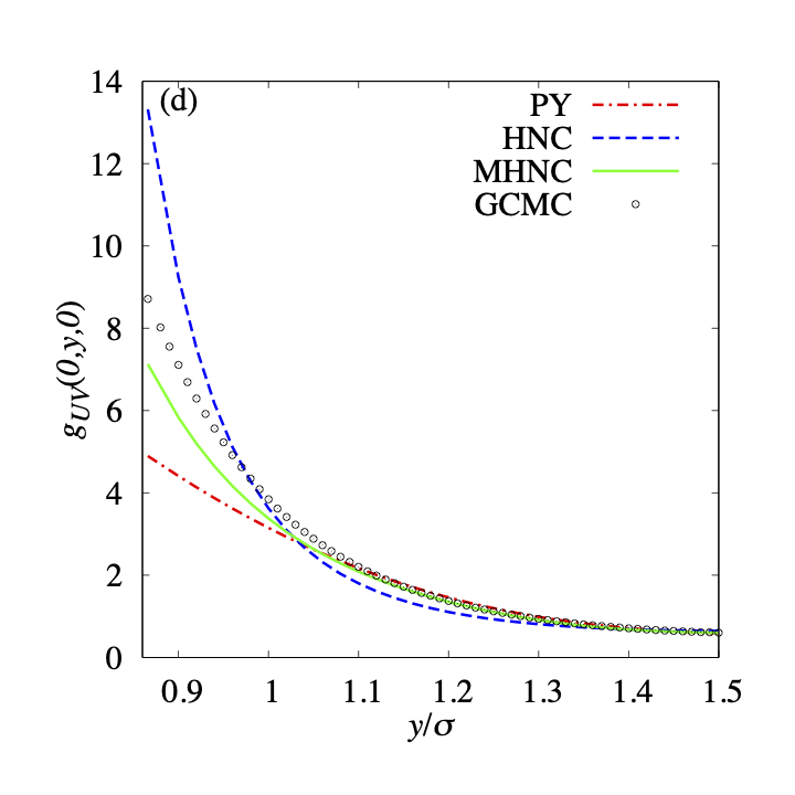
To quantitatively compare the results obtained by MC and closures we plot the spatial distribution along the $x$-axis $g_{UV}(x,0,0)$ and that along the $y$-axis $g_{UV}(0,y,0)$ in Fig.4. We chose two specific sections, namely most convex and concave sections, and plotted the distribution functions, namely $g_{UV}(x,0,0)$ and $g_{UV}(0,y,0)$.

Fig.4(a), (c) shows the solvent distribution around the most convex surface of the solute, namely $g_{UV}(x,0,0)$. The curvature of the solute particle is the same as that of the solvent particles. We can find the difference near the contact distance. The plot calculated by MHNC approximation almost agrees with that calculated by GCMC simulation.On the other hand, the HNC approximation overestimates, and the PY approximation underestimates the values near the solute surface. This agreement and these differences were also observed when the solute is a spherical one that has solvent particle size[5]. These results are reasonable because the curvature of the most convex surface of the solute is the same as that of the solvent particles.

On the other hand, the behaviors of $g(0,y,0)$ (Fig.4(b),(d)) deviate from those of $g(x,0,0)$. The differences from the GCMC simulation result become significant. At the contact distance, the value of the HNC approximation is about $1.5$ times, and the value of the PY approximation is about half of the GCMC result. Only the MHNC result keeps a small deviation from that for GCMC. The ratio of the contact value is about $0.85$. It indicates that MHNC closure gives a good approximation near the concave surface.

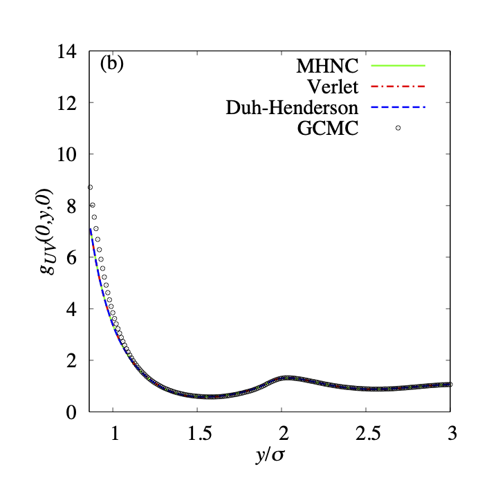
We also examine other bridge functions, namely, the Verlet bridge function and the Duh-Henderson bridge function. Fig.5 shows the results. We cannot distinguish the plots for the three bridge functions (Eqs.6, 7, 8). These bridge functions were also examined in the previous papers[57, 5]. When a spherical solute is immersed in the one-component hard sphere fluid, these bridge functions gave us adequate spatial distribution functions. Therefore, we discuss that the superiority of the MHNC closure is slight in the three closures. The superiority of the MHNC closure becomes significant when the value of $\gamma_{ij}(r)$ is negative and the absolute value $|\gamma_{ij}(r)|$ is large enough. As we mentioned in the previous paper [5], the function $\gamma_{ij}(r)$ does not have a large negative value in the case of a one-component solvent system. This is the reason for the small differences between the results calculated using three bridge functions. In the present study, this conclusion is maintained even when the surface of the solute is concave in the case of $g(0,y,0)$ (See Fig.5(b), (d)). The accuracies of the approximation with the bridge functions depend on the surface curvature of the solute. Fig.4 suggests that the accuracy near the convex surface of the solute is better than that near the concave surface. The spatial distribution functions $g(0,y,0)$ obtained using the approximation with the bridge functions are slightly smaller than that obtained using GCMC.

The validity of the closure can also be evaluated in terms of the three-body correlation. We discuss the triplet distribution functions. The triplet distribution functions $g^{(3)}(\mathbf{r_{1}},\mathbf{r_{2}},\mathbf{r_{3}})$ mean the reduced probability of finding three particles at positions $\mathbf{r_{1}}$, $\mathbf{r_{2}}$, and $\mathbf{r_{3}}$[73]. Then $g^{(3)}$ can be expressed by a triple product of the pair distribution functions $g^{(2)}$ which is called superposition approximation (SA)[74];

$$g^{(3)}_{\rm{SA}}(\mathbf{r_{1}},\mathbf{r_{2}},\mathbf{r_{3}})=g(\mathbf{r_{1}},\mathbf{r_{2}})g(\mathbf{r_{2}},\mathbf{r_{3}})g(\mathbf{r_{3}},\mathbf{r_{1}}).$$

(17)

When two particles are fixed at $\mathbf{r_{1}}$ and $\mathbf{r_{2}}$, reduced probability of finding a particle at position $\mathbf{r_{3}}$ is as follows using Eq.(17);

$$\begin{split}g_{\rm{SA}}(r_{12};\mathbf{r_{3}})&=g^{(3)}_{\rm{SA}}(\mathbf{r_{1}},\mathbf{r_{2}},\mathbf{r_{3}})/g(\mathbf{r_{1}},\mathbf{r_{2}})\\ &=g(\mathbf{r_{2}},\mathbf{r_{3}})g(\mathbf{r_{3}},\mathbf{r_{1}})\end{split}$$

(18)

where

$$r_{12}\equiv|\mathbf{r_{1}}-\mathbf{r_{2}}|.$$

(19)

Choosing the third Cartesian coordinate $\mathbf{r_{3}}=(x_{3},y_{3},z_{3})$ in Eq.(18) and setting $\mathbf{r_{1}}=(-0.5\sigma_{V},0,0)$ and $\mathbf{r_{2}}=(0.5\sigma_{V},0,0)$, we can calculate the spatial distribution function $g(x_{3},y_{3},z_{3})$ around contact dimer. Fig.6 shows the spatial distribution in $xy$ plane calculated from Eq.(18). Here, $g(\mathbf{r_{2}},\mathbf{r_{3}})$ and $g(\mathbf{r_{3}},\mathbf{r_{1}})$ are obtained using the radial distribution functions $g_{VV}(r)$ caluculated by GCMC simulation. Compared to Fig.3(a), the shape of density waves is in good agreement. This suggests that for simple solute models, the shape of the distribution of solvents can be estimated more or less accurately from the superposition approximation (SA).

Fig.7 shows the spatial distributions calculated using the MHNC approximation and the GCMC simulation with the results obtained using Eq.(18), namely SA. The features of functions$g_{UV}(x,0,0)$ are similar. The locations for the peaks and the minimums are almost the same. The numerical agreement between the GCMC and MHNC results is excellent (the contact value $g(1.5\sigma,0,0)=3.8935$(SA) and $3.5062$(GCMC), $3.3838$(MHNC) in Fig.4,7). On the other hand, the deviation of the SA results from the exact results is largest. However, the deviation is smaller than those obtained using PY or HNC ($g(1.5\sigma,0,0)=3.0473$(PY) and $4.3583$(HNC) in Fig.4).

We can find the same behavior as $g_{UV}(x,0,0)$ in $g_{UV}(0,y,0)$, and the differences become more significant. The first peaks of functions $g_{UV}(0,y,0)$ are higher than those of the $g_{UV}(x,0,0)$ because of the gain of the excluded volume at the contact position. Features of three functions$g_{UV}(0,y,0)$ for SA, MHNC, and GCMC are similar to each other again (the contact value $g(0,\sqrt{3}/2\sigma,0)=12.1041$(SA) and $8.7112$(GCMC), $7.1283$(MHNC) in Fig.4,7). The spatial distributions obtained by the SA with $g(r)$ obtained GCMC (or the MHNC approximation) are more accurate than those obtained using the HNC or the PY approximations ($g(0,\sqrt{3}/2\sigma,0)=4.8957$(PY) and $13.3187$(HNC) in Fig.4). It means that the SA using the accurate $g(r)$ is not bad despite the simplicity when we discuss the qualitative behavior of the distribution functions. On the other hand, the deviations from the SA results show the existence of multiple body correlations .

Here, we discuss the approximations based on the three-body effect. The SA includes only three independent pair correlations and ignores the effect of any of these pair correlations. Thus, the SA differs from the exact result when the third particle is in the neighborhood of the pair. To assess the actual three-body effect, we consider the ratio $g^{(3)}$ to the value of the SA(Eq.(18))[75, 76, 77]:

$$\Gamma(\mathbf{r_{1}},\mathbf{r_{2}},\mathbf{r_{3}})=\frac{g^{(3)}(\mathbf{r_{1}},\mathbf{r_{2}},\mathbf{r_{3}})}{g(\mathbf{r_{1}},\mathbf{r_{2}})g(\mathbf{r_{2}},\mathbf{r_{3}})g(\mathbf{r_{3}},\mathbf{r_{1}})}$$

(20)

which can be written as

$$\Gamma(r_{12};\mathbf{r_{3}})=\frac{g^{(3)}(r_{12};\mathbf{r_{3}})}{g(\mathbf{r_{2}},\mathbf{r_{3}})g(\mathbf{r_{3}},\mathbf{r_{1}})}.$$

(21)

If the SA were exact, the ratio $\Gamma$ should be unity. However, the calculated results are not unity except the SA.

Here we think of a contact dimer (particles 1 and 2) and a solvent particle 3. We define the ratio $\Gamma(\theta)=\Gamma(\mathbf{r_{3}})$ as a function of the angle $\theta$ enclosed by $\mathbf{r_{1}}-\mathbf{r_{2}}$ and $\mathbf{r_{3}}-\mathbf{r_{2}}$ (see Fig.8). The calculated results $\Gamma(\theta)$ at $|\mathbf{r_{3}}-\mathbf{r_{2}}|=\sigma$ for the HNC, PY, and MHNC closures are shown in Fig.9(a). The result of GCMC is also shown in the figure. First, we compare the SA and GCMC results. The exact result (GCMC) has two minimums around $60^{\circ}$ and $180^{\circ}$, and there is a peak around $120^{\circ}$. The first minimum at $60^{\circ}$ is caused by the overestimation of the SA. In other words, the numerator is smaller than the denominator in Eq.(21), which is the definition of $\Gamma$. Note the reference value, namely the denominator, is obtained by the SA in Eq.(21). Actually, particle 3 is stable at $60^{\circ}$ because of the reduction of excluded volume for the three particles. However, the SA does not contain the exclusion effect for particle 3 by particle 2. Thus, the peak of the solvent spatial distribution estimated by the SA becomes larger than the exact value at 60°. Therefore, the minimum at $60^{\circ}$ appears in the $\Gamma(\theta)$[78]. On the other hand, it seems that the second minimum at $180^{\circ}$ appears because of the reductions of the three-body effect at the configuration because the value smoothly approaches unity.

The peak for the GCMC result around $120^{\circ}$ appears because of the effect of the solvent located at $60^{\circ}$. The reduced spatial distribution has a high peak at $60^{\circ}$, and the peak value is much larger than the unity. As the probability of the existence of the solvent particle at $60^{\circ}$ becomes larger, the fourth particle at $120^{\circ}$ becomes stabler because of the reduction of the excluded volume caused by the adsorption. The SA does not include this three-body effect. Therefore, the probability of particle existence obtained using the GCMC at $120^{\circ}$ becomes larger than that of the estimation by the SA, and the peak around $120^{\circ}$ in Fig.9(a) appears.

Fig.9(a) also has the plots $\Gamma(\theta)$ for various closures, namely the PY, the HNC, and the MHNC closures. The functions $\Gamma(\theta)$ maintain the same features: two minimums at $60^{\circ}$ and $180^{\circ}$ and one peak at $120^{\circ}$. Quantitative deviations can be seen in contrast to the qualitative validity of these approximate three-body correlations. The deviation of the PY result from the exact result(the GCMC simulation) is the largest. Although the sign of deviation for the HNC result is opposite to that for the MHNC result, both differences are small. The exact result is also close to these two plots. The HNC result is very accurate in the plots $\Gamma(\theta)$. However, it does not mean that the HNC closure is very accurate in the calculation of the spatial distribution. It should be noted that the deviation of the spatial distribution function calculated by the HNC closure is larger than that calculated by the MHNC closure due to the large deviation of the two-body correlation from the exact solution.

Fig.9(b) shows the ratio $\Gamma(\mathbf{r_{3}})=\Gamma(x,y,z)$ as a function of the coordinate $(x,y,z)$. $\Gamma(0,y,0)$ at $y=\sqrt{3}/2$ is equivalent to $\Gamma(\theta)$ at $\theta=60^{\circ}$. The plots $\Gamma(0,y,0)$ oscillate, and the qualitative features of the plots in the Fig.9(b) are similar. Two deep minimums are located around $y=\sqrt{3}/2$ and $1.8$, and a clear peak is located at $1.3$. However, the deviation of the PY result from the exact results (GCMC) is the largest. The accuracies of the MHNC and the HNC approximations depend on the value $y$. Around $y=\sqrt{3}/2$ the HNC approximation is the most precise, while the MHNC becomes the most accurate around the first peak at $y=1.8$. However, the difference is not quantitively large.

Here, we discuss the detail of the differences of $\Gamma(0,y,0)$. The MHNC results evaluated well the value of $\Gamma(0,y,0)$ near the first and second peaks. These peak positions correspond to the bottoms (or minimums) of the distribution function $g(0,y,0)$, where SA underestimates. We calculated the $g(r)$ between two hard spheres immersed in a hard-sphere fluid using the MHNC approximation in the previous study[5]. The MHNC results showed very accurate first minimums in the $g(r)$. The accuracies were much better than that of HNC results. We can conclude that these share common features. Therefore, the evaluation of the distribution functions using the MHNC approximation is very accurate, even if we discuss the value around the minimum. On the other hand, the deviation of the HNC results for $\Gamma(0,y,0)$ around the first minimum is smaller than that of the MHNC result, although the deviations of the HNC results are much larger than those of the MHNC results in comparing the functions $g(r)$. In the case of the HNC results, both the numerator and the denominator of Eq.(21) are overestimated. In contrast, only the denominator for the MHNC result is very accurate in the calculation Eq.(21).

Fig.10 shows $\Gamma(\theta)$ and $\Gamma(0,y,0)$ of the GCMC result and three results for the various closures with bridge functions: the MHNC, the Verlet, and the Duh-Henderson bridge. The three closures have virtually the same results. We can find differences in $\Gamma(0,y,0)$ around $y=1.5\sigma_{V}$. The deviation of the Verlet bridge result from the exact result is the largest. However, the difference can be ignorable. Therefore, it is consistent with the agreement in the spatial distribution functions (see Fig.5).

It seems that the HNC approximation overestimates the pair correlation function due to the ignorance of the bridge function (see Eq. (5).) On the other hand, it has been shown that the pair correlation function given by the MHNC approximation is very accurate in the present system[5] . Furthermore, it is known that the pair correlation function also agrees well with MC if the bridge function was constructed to satisfy the thermodynamic consistency[79, 80]. The HNC approximation is also insufficient for thermodynamic consistency, but the results given by the MHNC approximation are automatically almost completely satisfied [81]. Therefore, we expected that the bridge function of the MHNC approximation is an adequate improvement and that the three-body correlation is also better than that calculated using the HNC approximation.

However, the superiority of some closures with a bridge function in the spatial distribution functions is not caused by the superiority of the three-body correlations. Here, the validity of the closure can also be evaluated in terms of the three-body correlation. Though the incorporation of the Verlet, Duh-Henderson, and Kinoshita bridge functions improves the pair correlation function, it does not necessarily lead to better results for the triplet distribution function. It is interesting to compare the results from the MC simulation and the OZ equations coupled with PY, HNC, and the three different closures in terms of the triplet distribution function. Under the present calculation conditions, the calculated results do not always mean that the MHNC approximation gives better results than the HNC approximation for the three-body correlation.

In the above calculation, configuration 1 (see Fig.11(a)) was adopted. We can also obtain the $\Gamma(\theta)$ by using configuration 2 (see Fig11(b)). In the method, a pair of two separate particles 1 and 3, fixed at ${\rm r}_{1}$ and ${\rm r}_{3}$ is immersed in the solvent particles. Thus, we calculate the spatial distribution function around them $g^{(3)}(r_{13};{\rm r}_{2})$ to obtain $\Gamma(\theta)$. In other word, $\Gamma(\theta)$ is calculated using the spatial distribution function at $\mathbf{r}_{2}$ when particle 1 and 3 is located at variable $\theta$. Then, $\Gamma(\theta)$ is written as

$$\Gamma(\theta)=\Gamma(r_{13};\mathbf{r_{2}})=\frac{g^{(3)}(r_{13};\mathbf{r_{2}})}{g(\mathbf{r_{1}},\mathbf{r_{2}})g(\mathbf{r_{2}},\mathbf{r_{3}})}.$$

(22)

Here, $g^{(3)}(r_{13};r_{2})$ is not the spatial distribution around a contact dimer solute. However, we can compare the $\Gamma(\theta)$ for configuration 2 with that for configuration 1. In Fig.12, we show the $\Gamma(\theta)$ results when the configuration 2 are adopted. The discrepancies between the exact GCMC result and the results for the various closures are much larger than those obtained using configuration 1 (Fig.9).

Here, we focus on the difference between the calculated results using the integral theories and the exact result using GCMC in Fig.12. In the case of exact results, the plot for configuration 2 is the same as that for configuration 1. In the case of configuration 1, we can also find the closure dependence (See Fig.9(a)). However, the dependence is much smaller than that for configuration 2 (See Fig.12). In the case of configuration 2, the value calculated using the MHNC is about $0.65$ when $\theta=180^{\circ}$. At $\theta=180^{\circ}$, since the three particles are aligned on a straight line, we expect that the three-body correlation effect is less apparent. It is because particle 3 is not strongly affected by particle 1 since particle 3 is located just behind particle 2 (See Fig.11). In fact, in the case of configuration 1, all plots converge to a value of about $0.9$ at $\theta=180^{\circ}$ (See Fig.9(a)). That is, in the case of configuration 1, especially when $\theta=180^{\circ}$, any approximation is close to the exact result. These results contrast with that of configuration 2. The poor approximation for the three-body correlation by closures is emphasized using configuration 2.

We discuss the reason for the difference between configurations 1 and 2. In a dilute system, the three-body correlation becomes weak, and $\Gamma$ goes to 1[41]. Conversely, the multi-body correlation becomes important in a dense fluid. Then, the value $\Gamma$ is expected to worsen as the local density becomes larger. As the overlap of the excluded volume increase, the configuration of the three particles becomes stable in the present packing fraction, and the local density of the third particle becomes high at the location. Therefore, the amount of the excluded volume overlap for the third particle, namely particle 2 for configuration 2, should correlate with the accuracy of the multi-body correlation.

For example, in the case of configuration 2, particle 2 contacts particles 1 and 3. Then, particle 2 has two excluded volume overlaps with particles 1 and 3 at any angle. Because of the large overlap amount, the local density of the third particle for configuration 2 is high, and the three-body correlation value deviates from the exact value in the entire range of $\theta=60^{\circ}$ to $180^{\circ}$ except the cross point near $\theta=130^{\circ}$ for HNC closure.

Let us discuss the validity of the above argument regarding the relationship between local density and three-body correlations based on the results for configuration 1. In the configuration, the excluded volume of particle 3 overlaps with both those of particles 1 and 2 near $\theta=60^{\circ}$. Therefore, at $60^{\circ}<\theta<120^{\circ}$, we can find differences between the exact calculation results and those calculated using the integral equation theories. On the other hand, when $120^{\circ}<\theta<180^{\circ}$, the excluded volume for particle 3 overlaps only that of particle 2. Since the overlap is less than that for $60^{\circ}<\theta<120^{\circ}$, the results of the integral equation theory roughly agree with the exact results. The above results coincide with the argument that the three-body correlation tends to be inaccurate in configurations where the local density of particles is high.

References

- [1] S. Asakura and F. Oosawa: J. Chem. Phys. 22,1255 (1954).
- [2] S. Asakura and F. Oosawa: J. Polym. Sci. 33,183 (1958).
- [3] A. Vrij: Pure and applied chemistry 48,471 (1976).
- [4] This effective interaction becomes purely enthalpic under isobaric condition. However, it does not mean that the effective interaction is driven by energy. The translational motion of depletants is the origin, even under the isobaric condition.
- [5] Y. Nakamura, S. Arai, M. Kinoshita, A. Yoshimori, and R. Akiyama: J. Chem. Phys. 151,044506 (2019).
- [6] R. Roth, B. Götzelmann, and S. Dietrich: Phys. Rev. Lett. 83,448 (1999).
- [7] R. Roth, R. Evans, A. Lang, and G. Kahl: J. Phys: Condens. Matter 14,12063 (2002).
- [8] Y. Rosenfeld: Phys. Rev. Lett. 63,980 (1989).
- [9] A. P. Minton: Curr. Opin. Biotechnol. 8,65 (1997).
- [10] A. B. Fulton: Cell 30,345 (1982).
- [11] D. S. Goodsell: Trends Biochem. Sci. 16,203 (1991).
- [12] A. R. Kinjo and S. Takada: Phys. Rev. E 66,031911 (2002).
- [13] A. R. Kinjo and S. Takada: Phys. Rev. E 66,051902 (2002).
- [14] R. J. Ellis and A. P. Minton: Nature 425,27 (2003).
- [15] D. Hall and A. P. Minton: Biochim. Biophys. Acta 1649,127 (2003).
- [16] R. Akiyama, Y. Karino, Y. Hakiwara, and M. Kinoshita: J. Phys. Soc. Jpn. 75,064804 (2006).
- [17] M. Kinoshita: Front. Biosci. 14,3419 (2009).
- [18] Y. Harano and M. Kinoshita: Chem. Phys. Lett. 399,342 (2004).
- [19] R. Roth, Y. Harano, and M. Kinoshita: Phys. Rev. Lett. 97,078101 (2006).
- [20] T. Yoshidome, M. Kinoshita, S. Hirota, N. Baden, and M. Terazima: J. Chem. Phys. 128,06B606 (2008).
- [21] A. Chiba, A. Oshima, and R.Akiyama: Langmuir 35,17177 (2019).
- [22] H. N. W. Lekkerkerker and R. Tuinier: Depletion interaction (Springer, 2011).
- [23] H. N. W. Lekkerkerker, W. C. K. Poon, P. N. Pusey, A. Stroobants, and P. B. Warren: Europhys. Lett. 20,559 (1992).
- [24] D. Frenkel and A. A. Louis: Phys. Rev. Lett. 68,3363 (1992).
- [25] M. Dijkstra, D. Frankel, and J. P. Hansen: J. Chem. Phys. 101,3179 (1994).
- [26] M. Dijkstra and D. Frankel: Phys. Rev. Lett. 72,298 (1994).
- [27] M. Dijkstra, R. van Roij, and R. Evans: Phys. Rev. Lett. 81,2268 (1998).
- [28] M. Dijkstra, R. van Roij, and R. Evans: Phys. Rev. Lett. 82,117 (1999).
- [29] M. Dijkstra, R. van Roij, and R. Evans: Phys. Rev. E 59,5744 (1999).
- [30] M. Dijkstra, J. M. Brader, and R.Evans: J. Phys.: Condens. Matter 11,10079 (1999).
- [31] M. Dijkstra, R. van Roji, R. Roth, and A. Fortini: Phys. Rev. E 73,041404 (2006).
- [32] G. Cinacchi, Y. Martínez-Ratón, L. Mederos, G. Navascués, A. Tani, and E. Velasco: J. Chem. Phys. 127,214501 (2007).
- [33] E. López-Sánchez, C. D. Estrada-Álvarez, G. Pérez-Ángel, J. M. Méndez-Alcaraz, P. González-Mozuelos, and R. Castañeda-Priego: J. Chem. Phys. 139,104908 (2013).
- [34] E. Velasco, G. Navascués, and L. Mederos: Phys. Rev. E 60,3158 (1999).
- [35] A. Suematsu, A. Yoshimori, and R. Akiyama: Europhys. Lett. 116,38004 (2016).
- [36] M. Kinoshita and F. Lado: Mol. Phys. 83,351 (1994).
- [37] R. Castañeda-Priego, A. Rodríguez-López, and J. M. Méndez-Alcaraz: J. Phys: Condens. Matter 15,S3393 (2003).
- [38] R. Roth and P. M. König: Pramana 64,971 (2005).
- [39] H. N. W. Lekkerkerker and B. Widom: Phys. A 285,483 (2000).
- [40] J. T. Lee and M. Robert: Phys. Rev. E 60,7198 (1999).
- [41] Y. Kubota and R. Akiyama: J. Phys. Soc. Jpn. 81,SA017 (2012).
- [42] M. Kinoshita: Biophys. Rev. 5,283 (2013).
- [43] Y. Harano and M. Kinoshita: Biophys. J 89,2701 (2005).
- [44] T. Yoshidome, Y. Harano, and M. Kinoshita: Phys. Rev. E 79,011912 (2009).
- [45] H. Oshima and M. Kinoshita: J. Chem. Phys. 138,245101 (2013).
- [46] H. Oshima and M. Kinoshita: J. Chem. Phys. 142,145103 (2015).
- [47] S. Murakami and M. Kinoshita: J. Chem. Phys. 144,125105 (2016).
- [48] S. Murakami, T. Hayashi, and M. Kinoshita: J.Chem. Phys. 146,055102 (2017).
- [49] M. Kinoshita: J. Chem. Phys. 116,3493 (2002).
- [50] R. Akiyama, Y. Karino, H. Obama, and A. Yoshifuku: PCCP 12,3096 (2010).
- [51] Y. Nakamura, A. Yoshimori, and R. Akiyama: J. Chem. Phys. 154,084501 (2021).
- [52] T. Yamada, T. Hayashi, S. Hikiri, N. Kobayashi, H. Yanagawa, M. Ikeguchi, M. Katahira, T. Nagata, and M. Kinoshita: J. Chem. Inf. Model. 59,3533 (2019).
- [53] M. Inoue, T. Hayashi, S. Hikiri, M. Ikeguchi, and M. Kinoshita: J. Mol. Liq. 317,114129 (2020).
- [54] N. Baden, S. Hirota, T. Takabe, N. Funasaki, and M. Terazima: J. Chem. Phys. 127,175103 (2007).
- [55] Y. Karino and R. Akiyama: Chem. Phys. Lett. 478,180 (2009).
- [56] M. Kinoshita: Chem. Phys. Lett. 353,259 (2002).
- [57] M. Kinoshita: J. Chem. Phys. 118,8969 (2003).
- [58] D. Chandler and J. D. Week: Phys. Rev. Lett. 25,149 (1970).
- [59] J. D. Week, D. Chandler, and H. C. Andersen: J. Chem. Phys. 54,5237 (1971).
- [60] D. Chandler, J. D. Week, and H. C. Andersen: Science 220,787 (1983).
- [61] Y. Yang-Xin and W. Jianzhong: J. Chem. Phys. 117,10156 (2002).
- [62] J.-P. Hansen and I. R. McDonald: Theory of simple liquids (Academic Press, Lodon, 1986).
- [63] P. Attard and G. N. Patey: J. Chem. Phys. 92,4970 (1990).
- [64] M. Kinoshita, S. Iba, K. Kuwamoto, and M. Harada: J. Chem. Phys. 105,7177 (1996).
- [65] M. Kinoshita and T. Hayashi: J. Molec. Liq. 247,403 (2017).
- [66] D. J. Adams: Mol. Phys. 28,1241 (1974).
- [67] D. J. Adams: Mol. Phys. 29,307 (1975).
- [68] L. Verlet: Mol. Phys. 41,183 (1980).
- [69] D. M. Duh and D. Henderson: J. Chem. Phys. 104,6742 (1996).
- [70] J. R. Schmidt and J. L. Skinner: J. Chem. Phys. 119,8062 (2003).
- [71] R. O. Sokolovskii, M. Thachuk, and G. N. Patey: J. Chem. Phys. 125,204502 (2006).
- [72] I. Nezbeda and J. Kolafa: Mol. Simulat. 5,391 (1991).
- [73] B. J. Alder: Phys. Rev. Lett. 12,317 (1964).
- [74] J. G. Kirkwood: J. Chem. Phys. 3,300 (1935).
- [75] Y. Uehara, Y. T. Lee, T. Ree, and T. H. Ree: J. Chem. Phys. 70,1884 (1979).
- [76] P. Attard and G. Stell: Chem. Phys. Lett. 189,128 (1992).
- [77] B. Bildstein and G. Kahl: J. Chem. Phys. 100,5882 (1994).
- [78] This minimum can also be explained in terms of the triplet overlap of the excluded volume. In the SA, the overlap of the excluded volume is double-counted.
- [79] F. J. Rogers and D. A. Young: Phys. Prev. A 30,999 (1984).
- [80] J. P. Hansen and G. Zerah: Phys. Lett. A 108,277 (1985).
- [81] T. Hayashi, H.Oshima, Y.Harano, and M.Kinoshita: J. Phys: Condens. Matter 28,344003 (2016).