Spatial Curvature and Thermodynamics
Abstract
Reasonable parametrizations of the current Hubble data set of the expansion rate of our homogeneous and isotropic universe, after suitable smoothing of these data, strongly suggest that the area of the apparent horizon increases irrespective of whether the spatial curvature of the metric is open, flat or closed. Put in another way, any sign of the spatial curvature appears consistent with the second law of thermodynamics.
keywords:
methods: data analysis – cosmological parameters – cosmology: observations – cosmology: theory1 Introduction
Homogeneous and isotropic cosmological models are most aptly described by the Friedmann-Lemaître-Robertson-Walker (FLRW) space-time metric,
| (1) |
The spatial curvature index, , indicates whether
the spatial part of the metric is open (negatively curved, i.e., hyperbolic),
flat, or closed (positively curved).
This constant index, like the scale factor , is
not a directly observable quantity. In principle, however, it can
be determined through the knowledge of the spatial curvature
density parameter, , which is
accessible to observation, albeit indirectly. Recent estimates of
the latter, assuming the universe correctly described by the
CDM model only suggests that its present absolute value
is small ( or less
(Komatsu
et al., 2011; Ade et al., 2014; Aghanim
et al., 2020; Vagnozzi et al., 2021a; Vagnozzi
et al., 2021b; Dhawan
et al., 2021; Park &
Ratra, 2019; Handley, 2021; Mukherjee &
Banerjee, 2022; Bel et al., 2022; Akarsu et al., 2023)). More recent measurements, not
based in the aforesaid model, hint that the universe may not be
flat (i.e., ) (Park &
Ratra, 2019; Handley, 2021; Mukherjee &
Banerjee, 2022; Bel et al., 2022). So, the sign of is rather uncertain.
Based on the history of the Hubble factor , (where
) it has been recently argued (Gonzalez-Espinoza & Pavón, 2019) that the
universe is a thermodynamic system in the sense that it satisfies the second
law of thermodynamics (the first law is guaranteed by Einstein
equations while the third law may not apply). As we shall see
soon, the possibilities and are consistent with
the second law while this is not so obvious for the third
possibility; in principle may or may not be compatible
with the second law. The aim of our study is to resolve this
uncertainty. To this end we shall resort to the 60 data
currently available alongside their confidence
intervals, the parametrized graph of this history after smoothing
the data set by a Gaussian Process (Rasmussen &
Williams, 2005), the FLRW
metric and the expression of the area of the apparent horizon (Eq.
(2) below). As it turns out, the possibility
(open spatial sections) appears also compatible with the second
law of thermodynamics. The paper is organized as follows: In
section 2 we write the second law at cosmic scales in terms of
the deceleration parameter and . In section 3 we
present the data set and the smoothing process. In section 4
we introduce four parametrizations of the Hubble factor and study
whether they are compatible with the second law. In section 5 we
consider the impact of the Hubble constant priors on our results.
Finally, in section 6 we summarize our findings.
As usual, a subindex zero attached at any given quantity indicates that the quantity is to be evaluated at the present epoch. Likewise, we recall, for future convenience, that after fixing , the redshift, , of any given luminous source is related to the corresponding scale factor by . In our units .
2 The second law
| [km Mpc-1 s-1] | Ref. | |
|---|---|---|
| 0.09 | 69 12 | Stern et al. (2010) |
| 0.17 | 83 8 | |
| 0.27 | 77 14 | |
| 0.4 | 95 17 | |
| 0.48 | 97 62 | |
| 0.88 | 90 40 | |
| 0.9 | 117 23 | |
| 1.3 | 168 17 | |
| 1.43 | 177 18 | |
| 1.53 | 140 14 | |
| 1.75 | 202 40 | |
| 0.1797 | 75 4 | Moresco et al. (2012) |
| 0.1993 | 75 5 | |
| 0.3519 | 83 14 | |
| 0.5929 | 104 13 | |
| 0.6797 | 92 8 | |
| 0.7812 | 105 12 | |
| 0.8754 | 125 17 | |
| 1.037 | 154 20 | |
| 0.07 | 69.0 19.6 | Zhang et al. (2014) |
| 0.12 | 68.6 26.2 | |
| 0.2 | 72.9 29.6 | |
| 0.28 | 88.8 36.6 | |
| 1.363 | 160.0 33.6 | Moresco (2015) |
| 1.965 | 186.5 50.4 | |
| 0.3802 | 83.0 13.5 | Moresco et al. (2016) |
| 0.4004 | 77.0 10.2 | |
| 0.4247 | 87.1 11.2 | |
| 0.4497 | 92.8 12.9 | |
| 0.4783 | 80.9 9 | |
| 0.47 | 89 49.6 | Ratsimbazafy et al. (2017) |
| 0.75 | 98.8 33.6 | Borghi et al. (2022) |
Given the strong connection between gravity and
thermodynamics (Bekenstein, 1974, 1975; Hawking, 1974; Jacobson, 1995; Padmanabhan, 2005), it is natural
to expect that the universe behaves as a normal thermodynamic
system (Gonzalez-Espinoza & Pavón, 2019) whereby it must tend to a state of
maximum entropy in the long run (Radicella &
Pavon, 2012; Pavon &
Radicella, 2013).
A basic standpoint is that the entropy of the universe
is dominated by entropy of the cosmic horizon. In fact its
entropy () exceeds by far the combined entropies
of super-massive black holes, the cosmic
microwave background radiation, the neutrino sea, etc (Egan &
Lineweaver, 2010). As
cosmic horizon, we take the apparent horizon rather than other
possible choices, since the laws of thermodynamics are fulfilled on
it (Wang
et al., 2006). Its entropy (proportional to its area) is given by
(Bak & Rey, 2000; Cai, 2008), with as the radius of the horizon.
Obviously, the area of the apparent horizon,
| (2) |
depends on the Hubble factor and spatial curvature.
By the second law of thermodynamics , thus
| (3) |
where the prime indicates .
The above inequality tells us: if is or has
been positive at any stage of cosmic expansion (excluding,
possibly, the pre-Planckian era), then ,
may, in principle, be compatible with any sign of , and
the possibilities and are consistent with the
second law. In particular the data analysis carried out by the 2018
Planck mission produced the 99 probability region
on the spatial curvature parameter
(Aghanim
et al., 2020). Note that this bound on is fully
compatible with the second law because it corresponds
to the possibility . However, the third possibility, ,
may or may not be compatible.
| [km Mpc-1 s-1] | [Mpc] | Ref. | |
| 0.24 | 79.69 2.99 | 153.3 | Gaztanaga et al. (2009) |
| 0.34 | 83.8 3.66 | ||
| 0.43 | 86.45 3.97 | ||
| 0.44 | 82.6 7.8 | Blake et al. (2012) | |
| 0.6 | 87.9 6.1 | ||
| 0.73 | 97.3 7 | ||
| 0.3 | 81.7 6.22 | 152.76 | Oka et al. (2014) |
| 0.35 | 82.7 9.1 | 152.76 | Chuang & Wang (2013) |
| 0.57 | 96.8 3.4 | 147.28 | Anderson et al. (2014) |
| 0.31 | 78.17 4.74 | 147.74 | Wang et al. (2017) |
| 0.36 | 79.93 3.39 | ||
| 0.40 | 82.04 2.03 | ||
| 0.44 | 84.81 1.83 | ||
| 0.48 | 87.79 2.03 | ||
| 0.52 | 94.35 2.65 | ||
| 0.56 | 93.33 2.32 | ||
| 0.59 | 98.48 3.19 | ||
| 0.64 | 98.82 2.99 | ||
| 0.38 | 81.5 1.9 | 147.78 | Alam et al. (2017) |
| 0.51 | 90.4 1.9 | ||
| 0.61 | 97.3 2.1 | ||
| 0.978 | 113.72 14.63 | 147.78 | Zhao et al. (2019) |
| 1.23 | 131.44 12.42 | ||
| 1.526 | 148.11 12.71 | ||
| 1.944 | 172.63 14.79 | ||
| 2.33 | 224 8 | 147.33 | Bautista et al. (2017) |
| 2.34 | 222 7 | 147.7 | Delubac et al. (2015) |
| 2.36 | 226 8 | 147.49 | Font-Ribera et al. (2014) |
The inequality can be recast as
| (4) |
where is the
deceleration parameter.
Equation (4) expresses the second law
of thermodynamics at cosmic scales (Gonzalez-Espinoza & Pavón, 2019).

To see that it is perfectly reasonable, let us assume the universe dominated by a perfect fluid of energy density and hydrostatic pressure . The corresponding Einstein equations can be written as,
| (5) |
If the fluid is dust (), one has ,
and these equations lead to .
If the second law holds, i.e., ,
it follows that which is consistent with the fact that
a pressureless matter dominated universe decelerates ().
By contrast, should the second law not hold, , the absurd result (namely, zero less than a
negative quantity), would follow.
Likewise, if the equation of state of the fluid filling
the universe were with the expression
also proves to be consistent with the
corresponding sign of the deceleration parameter and not so, if . Values of lower that correspond to
phantom fields. As is well known these fields are unstable both
classically (Dabrowski, 2015) and quantum
mechanically111Should be positive, the FLRW universe
could neither be flat nor open, just closed () which
would be puzzling in view of the current data that clearly allow
for . (Cline
et al., 2004).
Further, by combining the Friedmann equation in the case of a universe dominated by pressureless matter, the cosmological constant and spatial curvature with the acceleration equation (5.b), we obtain
| (6) |
The latter can be rewritten as
| (7) |
which makes apparent the reasonableness of the expression . Moreover, the above shows the compatibility of the said expression with general relativity.

(a) M1

(c) M3

(b) M2
3 Hubble data set and smoothing process
Our data set consists of: recent 32 cosmic
chronometer (CC) measurements, presented in Table
1, which do not assume any particular
cosmological model, and the 28 measurements from
baryon acoustic oscillations (BAO) from different galaxy surveys,
listed in Table 2. In both cases, the datasets are given
with their confidence interval. Because the BAO measurements are not
entirely model-independent, particularly due to the assumption of
a fiducial radius of the comoving sound horizon,
, we adopted a full marginalization over the
GP hyperparameter space (see below) with the comoving sound
horizon at drag epoch for the BAO data set as free
parameter. This results in a model-independent Hubble data set
from CC and the calibrated BAO.
| Sq.Exp | |||||
|---|---|---|---|---|---|
| Mat.7/2 | |||||
| Cauchy | |||||
| R.Quad |
| Sq.Exp | ||||||
|---|---|---|---|---|---|---|
| Mat.7/2 | ||||||
| Cauchy | ||||||
| R.Quad |
| Sq.Exp | |||||
|---|---|---|---|---|---|
| Mat.7/2 | |||||
| Cauchy | |||||
| R.Quad |


As is apparent, a handful of data are afflicted by
a rather large confidence intervals whence some statistically
founded smoothing process must be applied to the full data set to
arrive to sensible results. This is why we resort to the
machine-learning model Gaussian Process (GP) which infers a
function from labelled training data
(Rasmussen &
Williams, 2005; Seikel
et al., 2012), and reconstruct the Hubble
diagram as a function of the scale factor. The said process is
able to reproduce an ample range of behaviors with just a few
parameters and allows a Bayesian interpretation (Zhao
et al., 2008).
Then, after smoothing the Hubble data set, we constrain the free
parameters that enter the proposed parametric expressions (Eqs.
(10), (13) and
(15), below) of the history of the Hubble
factor and check whether the corresponding curves, , are
consistent with the second law. That is to say, whether they
comply with the inequality .
To undertake the GP, we consider the squared exponential (SqExp hereafter), Matérn 7/2 (Mat72 hereafter), Cauchy and rational quadratic (R.Quad hereafter) covariance functions,
| (8) |
(also called “kernels") where , and are the hyperparameters. Throughout this work, we assume a zero mean
function to characterize the GP. We investigate if the different covariance functions lead to significant differences
in the results222For details on GP, visit http://www.gaussianprocess.org.
We adopt a python implementation of the ensemble sampler for MCMC, the emcee333https://github.com/dfm/emcee, introduced by Foreman-Mackey et al. (2013). The two dimensional confidence contours showing the uncertainties along with the one dimensional marginalized posterior probability distributions, are shown in Fig. 1 with the help of the GetDist444https://github.com/cmbant/getdist module of python, developed by Lewis (2019).


4 Parametrizations
In this section we study whether hyperbolic, i.e., open,
spatial sections (which correspond to ) are compatible
with the second law of thermodynamics as expressed by Eq,
(4). To this end we consider three
parametrizations (equations (10), (13)
and (15), below) of the history of the Hubble
factor and use the corresponding parameter values obtained after
the smoothing of the Hubble data (tables 3,
4 and 5 for the first, second
and third parametrizations, respectively555In these tables
is the scale factor at which the transition from
deceleration to acceleration occurs.). Figure 2 shows
the contour plots of the different parameters occurring the three
parametrizations. Then we check whether the corresponding curves,
, comply with the inequality (4). These curves
are shown in Fig. 3.
We express as
| (9) |
with the upper bound on the likely
present value of the spatial curvature parameter assuming ,
see
Komatsu
et al. (2011); Ade et al. (2014); Park &
Ratra (2019); Handley (2021); Mukherjee &
Banerjee (2022); Bel et al. (2022).
In the cases considered below . The analysis of the fourth parametrization does not call for a
numerical study.
Before going any further, it is worthwhile to note that since and that () when the universe is decelerating (accelerating), the said inequality cannot be violated when the universe is decelerating.
4.1 First parametrization
A reasonable and simple parametrization of the Hubble factor in an ever-expanding FLRW universe, regardless of the spatial curvature (M1 hereafter), is
| (10) |
where and are free parameters to be fitted to the data
by means of the GP method.
Since there is deceleration when and acceleration when . On the other hand, recalling that is given by (9), and after setting , Eq. (4) boils down to
| (11) |
which can be rewritten as
| (12) |
Using the best fit values of and , shown in Table 3 corresponding to each kernel, we find that stays above in the full range, , of the scale factor covered by the data as shown in Fig. 4. Thus Eq. (12) is satisfied, i.e., the curve of the first parametrization respects, by a comfortable margin, the second law of thermodynamics also if .
4.2 Second parametrization
A somewhat less simple parametrization (M2 hereafter) is
| (13) |
This one contains three free parameters, namely, , and , to be fitted to the data. Proceeding as before we can write,
| (14) |
4.3 Third parametrization
Similarly, consider the expression (M3 hereafter) for the Hubble rate
| (15) |
where and are free parameter to be fit to the data.
As before, resorting to the best fit values of the free parameters as given in table 5 it is seen, that the above equation is satisfied (and consequently Eq. (4) as well) by a generous margin in the whole interval of the scale factor observationally accessible, as shown in Fig. 4. Once again, the second law is respected even if .

(a) M1

(c) M3
(b) M2
| Prior | |||||
|---|---|---|---|---|---|
| P | |||||
| F | |||||
| R |
| Prior | ||||||
|---|---|---|---|---|---|---|
| P | ||||||
| F | ||||||
| R |
| Prior | |||||
|---|---|---|---|---|---|
| P | |||||
| F | |||||
| R |


4.4 Fourth parametrization
Consider the expression for the Hubble factor inspired in the CDM model
| (17) |
where , and are free parameters. Following parallel steps to the previous cases, we write , that is to say
| (18) |
It is immediately seen that Eq. (4) is satisfied for whatever value of the scale factor and consequently the second law as well.
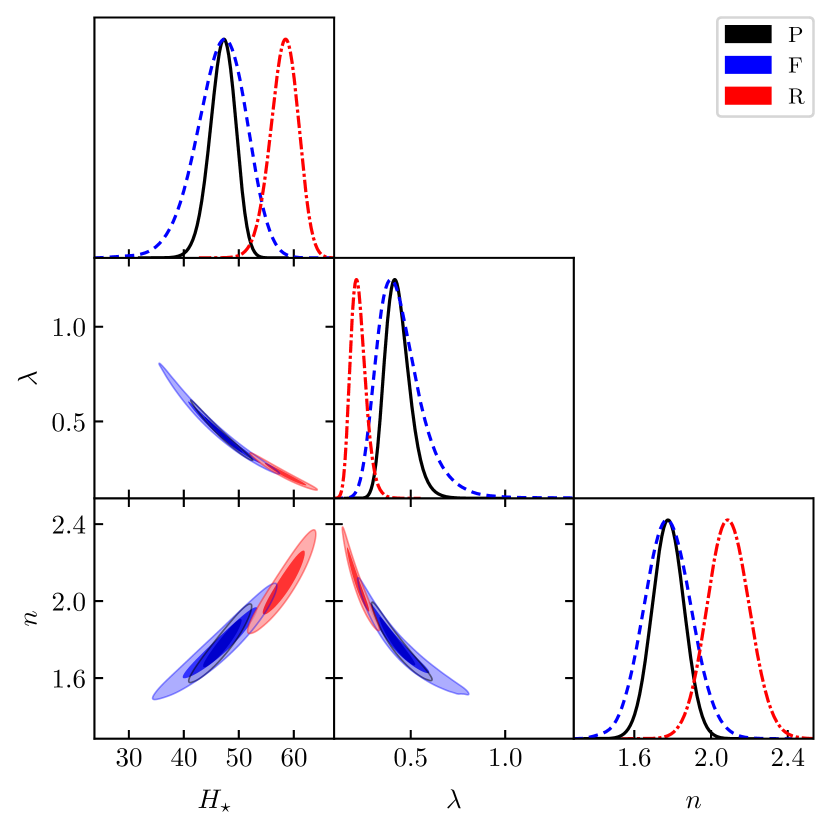
5 Effect of priors
We further examine to what extent (if at all) the rising
tension between the local measurements of the Hubble constant
(Riess et al., 2022; Freedman, 2021), and its inferred values via an
extrapolation of data on the early universe (Aghanim
et al., 2020)
affects our results.
To this end we consider the local measurements by
the SH0ES team [ = km Mpc-1
s-1 (R hereafter)], the updated TRGB calibration from
the Carnegie Supernova Project [ = km Mpc-1 s-1 (F hereafter)], and the
inferred value via an extrapolation of data on the early universe
by the Planck survey [ = km
Mpc-1 s-1 (P hereafter)], respectively. We assume
Gaussian prior distributions with the mean and variances
corresponding to the best-fit and confidence interval
reported about values.
Fig. 5 shows the contour plots of the different parameters
occurring in the three parametrizations, on assuming these values. The
constraints on the parameter values are given in Tables 6,
7, and 8, for the first, second and third
parametrizations. The corresponding and curves are shown in
Figs. 6 and 7, respectively.
We can conclude this section by saying that our overall result, that the constrain is satisfied even if , is not affected whether we take the value from the local measurements or the one obtained from extrapolating the precise data drawn from the cosmic microwave background radiation.
6 Concluding remarks
The second law of thermodynamics applied to our
expanding FLRW universe implies that the area of its apparent
horizon cannot decrease, i.e., . This, in its
turn, dictates . Since in absence of phantom
fields, which are unstable, leads to two possibilities, namely,
and , result immediately compatible with the second
law. The third possibility, , may or may not be
compatible with it. Here we resorted to the set of observational
data regarding the evolution of the Hubble factor to discern
whether the said law is satisfied when . So, with the
help of the non-parametric Gaussian Process we smoothed the set of
currently available data of the Hubble factor and introduced
four different parametrizations of the ensuing curve, .
After using the latter to constrain the free parameters entering
the first three parametrizations (the fourth one was not in need
of a numerical study), we examined whether the resulting
expressions, with the curvature index fixed to , satisfy
Eq. (4). As it turned out, all of them did (Fig.
4 and Eq. (18)). Further, a
quick inspection of the said expressions shows that they also
comply with Eq. (4) in the limit .
Therefore, we are led to conclude that the evolution of FLRW
universes with open spatial sections does not appear to conflict
with the second law of thermodynamics. Regrettably, a final
verdict cannot be attained at this stage since currently we have
no cosmological model that deserves our unreserved confidence. In
fact, the most reliable model, the so-called “concordance model",
is afflicted by some drawbacks whose relevance may not be small
(Perivolaropoulos &
Skara, 2022; Di Valentino, 2022). This is why we did resort to
parametrize the Hubble factor rather than taking it from any
given model.
One may argue that this conclusion could be reached from Eq.(7) straightaway. However this is not so because that equation only concerns the adiabatic evolution of the fluid that sources the gravitational field. Further, the second law does not enter its derivation whereby it cannot be ascertained whether it is respected or violated.
Acknowledgments
PM thanks ISI Kolkata for financial support through Research Associateship.
Data Availability
Authors can confirm that all relevant source data are included in the article. The data sets generated during and/or analysed during this study are available from the corresponding author on reasonable request.
References
- Ade et al. (2014) Ade P. A. R., et al., 2014, Astron. Astrophys., 571, A16
- Aghanim et al. (2020) Aghanim N., et al., 2020, Astron. Astrophys., 641, A6
- Akarsu et al. (2023) Akarsu O., Di Valentino E., Kumar S., Ozyigit M., Sharma S., 2023, Phys. Dark Univ., 39, 101162
- Alam et al. (2017) Alam S., et al., 2017, Mon. Not. Roy. Astron. Soc., 470, 2617
- Anderson et al. (2014) Anderson L., et al., 2014, Mon. Not. Roy. Astron. Soc., 441, 24
- Bak & Rey (2000) Bak D., Rey S.-J., 2000, Class. Quant. Grav., 17, L83
- Bautista et al. (2017) Bautista J. E., et al., 2017, Astron. Astrophys., 603, A12
- Bekenstein (1974) Bekenstein J. D., 1974, Phys. Rev. D, 9, 3292
- Bekenstein (1975) Bekenstein J. D., 1975, Phys. Rev. D, 12, 3077
- Bel et al. (2022) Bel J., Larena J., Maartens R., Marinoni C., Perenon L., 2022, JCAP, 09, 076
- Blake et al. (2012) Blake C., et al., 2012, Mon. Not. Roy. Astron. Soc., 425, 405
- Borghi et al. (2022) Borghi N., Moresco M., Cimatti A., 2022, Astrophys. J. Lett., 928, L4
- Cai (2008) Cai R.-G., 2008, Progress of Theoretical Physics Supplement, 172, 100
- Chuang & Wang (2013) Chuang C.-H., Wang Y., 2013, Mon. Not. Roy. Astron. Soc., 435, 255
- Cline et al. (2004) Cline J. M., Jeon S., Moore G. D., 2004, Phys. Rev. D, 70, 043543
- Dabrowski (2015) Dabrowski M. P., 2015, Eur. J. Phys., 36, 065017
- Delubac et al. (2015) Delubac T., et al., 2015, Astron. Astrophys., 574, A59
- Dhawan et al. (2021) Dhawan S., Alsing J., Vagnozzi S., 2021, Mon. Not. Roy. Astron. Soc., 506, L1
- Di Valentino (2022) Di Valentino E., 2022, Universe, 8, 399
- Egan & Lineweaver (2010) Egan C. A., Lineweaver C., 2010, Astrophys. J., 710, 1825
- Font-Ribera et al. (2014) Font-Ribera A., et al., 2014, JCAP, 05, 027
- Foreman-Mackey et al. (2013) Foreman-Mackey D., Hogg D. W., Lang D., Goodman J., 2013, Publ. Astron. Soc. Pac., 125, 306
- Freedman (2021) Freedman W. L., 2021, Astrophys. J., 919, 16
- Gaztanaga et al. (2009) Gaztanaga E., Cabre A., Hui L., 2009, Mon. Not. Roy. Astron. Soc., 399, 1663
- Gonzalez-Espinoza & Pavón (2019) Gonzalez-Espinoza M., Pavón D., 2019, Mon. Not. Roy. Astron. Soc., 484, 2924
- Handley (2021) Handley W., 2021, Phys. Rev. D, 103, L041301
- Hawking (1974) Hawking S. W., 1974, Nature, 248, 30
- Jacobson (1995) Jacobson T., 1995, Phys. Rev. Lett., 75, 1260
- Komatsu et al. (2011) Komatsu E., et al., 2011, Astrophys. J. Suppl., 192, 18
- Lewis (2019) Lewis A., 2019, arXiv.1910.13970
- Moresco et al. (2012) Moresco M., Cimatti A., Jimenez R., Pozzetti L., et al., 2012, JCAP, 2012, 006
- Moresco (2015) Moresco M., 2015, Mon. Not. Roy. Astron. Soc., 450, L16
- Moresco et al. (2016) Moresco M., et al., 2016, JCAP, 05, 014
- Mukherjee & Banerjee (2022) Mukherjee P., Banerjee N., 2022, Phys. Rev. D, 105, 063516
- Oka et al. (2014) Oka A., Saito S., Nishimichi T., Taruya A., Yamamoto K., 2014, Mon. Not. Roy. Astron. Soc., 439, 2515
- Padmanabhan (2005) Padmanabhan T., 2005, Phys. Rept., 406, 49
- Park & Ratra (2019) Park C.-G., Ratra B., 2019, Astrophys. Space Sci., 364, 134
- Pavon & Radicella (2013) Pavon D., Radicella N., 2013, Gen. Rel. Grav., 45, 63
- Perivolaropoulos & Skara (2022) Perivolaropoulos L., Skara F., 2022, New Astron. Rev., 95, 101659
- Radicella & Pavon (2012) Radicella N., Pavon D., 2012, Gen. Rel. Grav., 44, 685
- Rasmussen & Williams (2005) Rasmussen C. E., Williams C. K. I., 2005, Gaussian Processes for Machine Learning. The MIT Press, doi:10.7551/mitpress/3206.001.0001, https://doi.org/10.7551/mitpress/3206.001.0001
- Ratsimbazafy et al. (2017) Ratsimbazafy A. L., Loubser S. I., Crawford S. M., Cress C. M., Bassett B. A., Nichol R. C., Väisänen P., 2017, Mon. Not. Roy. Astron. Soc., 467, 3239
- Riess et al. (2022) Riess A. G., et al., 2022, Astrophys. J. Lett., 934, L7
- Seikel et al. (2012) Seikel M., Clarkson C., Smith M., 2012, JCAP, 06, 036
- Stern et al. (2010) Stern D., Jimenez R., Verde L., Kamionkowski M., Stanford S. A., 2010, JCAP, 02, 008
- Vagnozzi et al. (2021a) Vagnozzi S., Di Valentino E., Gariazzo S., Melchiorri A., Mena O., Silk J., 2021a, Phys. Dark Univ., 33, 100851
- Vagnozzi et al. (2021b) Vagnozzi S., Loeb A., Moresco M., 2021b, Astrophys. J., 908, 84
- Wang et al. (2006) Wang B., Gong Y., Abdalla E., 2006, Phys. Rev. D, 74, 083520
- Wang et al. (2017) Wang Y., et al., 2017, Mon. Not. Roy. Astron. Soc., 469, 3762
- Zhang et al. (2014) Zhang C., Zhang H., Yuan S., Zhang T.-J., Sun Y.-C., 2014, Res. Astron. Astrophys., 14, 1221
- Zhao et al. (2019) Zhao G.-B., et al., 2019, Mon. Not. Roy. Astron. Soc., 482, 3497
- Zhao et al. (2008) Zhao K., Popescu S., Zhang X., 2008, Photogrammetric Engineering & Remote Sensing, 74, 1223