Sparsity-Exploiting Distributed Projections onto a Simplex
Abstract
Projecting a vector onto a simplex is a well-studied problem that arises in a wide range of optimization problems. Numerous algorithms have been proposed for determining the projection; however, the primary focus of the literature has been on serial algorithms. We present a parallel method that decomposes the input vector and distributes it across multiple processors for local projection. Our method is especially effective when the resulting projection is highly sparse; which is the case, for instance, in large-scale problems with i.i.d. entries. Moreover, the method can be adapted to parallelize a broad range of serial algorithms from the literature. We fill in theoretical gaps in serial algorithm analysis, and develop similar results for our parallel analogues. Numerical experiments conducted on a wide range of large-scale instances, both real-world and simulated, demonstrate the practical effectiveness of the method.
1 Introduction
Given a vector , we consider the following projection of :
| (1) |
where is a scaled standard simplex parameterized by some scaling factor ,
1.1 Applications
Projection onto a simplex can be leveraged as a subroutine to determine projections onto more complex polyhedra. Such projections arise in numerous settings such as: image processing, e.g. labeling (Lellmann et al. 2009), or multispectral unmixing (Bioucas-Dias et al. 2012); portfolio optimization (Brodie et al. 2009); and machine learning (Blondel et al. 2014). As a particular example, projection onto a simplex can be used to project onto the parity polytope (Wasson et al. 2019):
| (2) |
where is a -dimensional parity polytope:
Projection onto the parity polytope arises in linear programming (LP) decoding (Liu and Draper 2016, Barman et al. 2013, Zhang and Siegel 2013, Zhang et al. 2013, Wei et al. 2015), which is used for signal processing.
Another example is projection onto a ball:
| (3) |
Duchi et al. (2008) demonstrate that the solution to this problem can be easily recovered from projection onto a simplex. Furthermore, projection onto a ball can, in turn, be used as a subroutine in gradient-projection methods (see e.g. van den Berg (2020)) for a variety of machine learning problems that use penalty, such as: Lasso (Tibshirani 1996); basis-pursuit denoising (Chen et al. 1998, van den Berg and Friedlander 2009, van den Berg 2020); sparse representation in dictionaries (Donoho and Elad 2003); variable selection (Tibshirani 1997); and classification (Barlaud et al. 2017).
Finally, we note that methods for projection onto the scaled standard simplex and ball can be extended to projection onto the weighted simplex and weighted ball (Perez et al. 2020a) (see Section B.2). Projection onto the weighted simplex can, in turn, be used to solve the continuous quadratic knapsack problem (Robinson et al. 1992). Moreover, regularization can be handled by iteratively solving weighted projections (Candès et al. 2008, Chartrand and Yin 2008, Chen and Zhou 2014).
1.2 Contributions
This paper presents a method to decompose the projection problem and distribute work across (up to ) processors. The key insight to our approach is captured by Proposition 3.4: the projection of any subvector of onto a simplex (in the corresponding space with scale factor ) will have zero-valued entries only if the full-dimension projection has corresponding zero-valued entries. The method can be interpreted as a sparsity-exploiting distributed preprocessing method, and thus it can be adapted to parallelize a broad range of serial projection algorithms. We furthermore provide extensive theoretical and empirical analyses of several such adaptations. We also fill in gaps in the literature on serial algorithm complexity. Our computational results demonstrate significant speedups from our distributed method compared to the state-of-the-art over a wide range of large-scale problems involving both real-world and simulated data.
Our paper contributes to the limited literature on parallel computation for large-scale projection onto a simplex. Most of the algorithms for projection onto a simplex are for serial computing. Indeed, to our knowledge, there is only one published parallel method, and one distributed method for projection problem (1). Wasson et al. (2019) parallelize a basic sort and scan (specifically prefix sum) approach–a method that we use as a benchmark in our experiments. We also develop a modest but practically significant enhancement to their approach. Iutzeler and Condat (2018) propose a gossip-based distributed ADMM algorithm for projection onto a Simplex. In this gossip-based setup, one entry of is given to each agent (e.g. processor), and communication is restricted according to a particular network topology. This differs fundamentally from our approach both in context and intended use, as we aim to solve large-scale problems and moreover our method can accommodate any number of processors up to .
The remainder of the paper is organized as follows. Section 2 describes serial algorithms from the literature and develops new complexity results to fill in gaps in the literature. Section 3 develops parallel analogues of the aforementioned algorithms using our novel distributed method. Section 4 extends these parallelized algorithms to various applications of projection onto a simplex. Section 5 describes computational experiments. Section 6 concludes. Note that all appendices, mathematical proofs, as well as our code and data can be found in the online supplement.
2 Background and Serial Algorithms
This section begins with a presentation of some fundamental results regarding projection onto a simplex, followed by analysis of serial algorithms for the problem, filling in various gaps in the literature. The final subsection, Section 2.5, provides a summary. Note that, for the purposes of average case analysis, we assume uniformly distributed inputs, are )—a typical choice of distribution in the literature (e.g. Condat (2016)).
2.1 Properties of Simplex Projection
KKT conditions characterize the unique optimal solution to problem (1):
Proposition 2.1 (Held et al. (1974)).
For a vector and a scaled standard simplex , there exists a unique such that
| (4) |
where .
Hence, (1) can be reduced to a univariate search problem for the optimal pivot . Note that the nonzero (positive) entries of correspond to entries where . So for a given value and the index set , we denote the active index set
as the set containing all indices of active elements where . Now consider the following function, which will be used to provide an alternate characterization of :
| (5) |
Corollary 2.2.
For any such that , we have
The sign of only changes once, and is its unique root. These results can be leveraged to develop search algorithms for , which are presented next. This corollary and the use of is our own contribution, as we have found it a convenient organizing principle for the sake of exposition We note, however, that the root finding framework has been in use in the more general constrained quadratic programming literature (see (Cominetti et al. 2014, Equation 5) and (Dai et al. 2006, Section 2, Paragraph 2)).
2.2 Sort and Scan
Observe that only the greatest terms of are indexed in . Now suppose we sort in non-increasing order:
We can sequentially test these values in descending order, etc. to determine . In particular, from Corollary 2.2 we know there exists some such that . Thus the projection must have active elements, and since , we have . We also note that, rather than recalculating at each iteration, one can keep a running cumulative/prefix sum or scan of as increments.
The bottleneck is sorting, as all other operations are linear time; for instance, QuickSort executes the sort with average complexity and worst-case , while MergeSort has worst-case (see, e.g. (Bentley and McIlroy 1993)). Moreover, non-comparison sorting methods can achieve (see, e.g. (Mahmoud 2000)), albeit typically with a high constant factor as well as dependence on the bit-size of .
2.3 Pivot and Partition
Sort and Scan begins by sorting all elements of , but only the greatest terms are actually needed to calculate . Pivot and Partition, proposed by Duchi et al. (2008), can be interpreted as a hybrid sort-and-scan that attempts to avoid sorting all elements. We present as Algorithm 2 a variant of this method approach given by Condat (2016).
The algorithm selects a pivot , which is intended as a candidate value for ; the corresponding value is calculated. From Corollary 2.2, if , then and so ; consequently, a new pivot is chosen in the (tighter) interval , which is known to contain . Otherwise, if , then , and so we can find a new pivot , where is the complement set. Repeatedly selecting new pivots and creating partitions in this manner results in a binary search to determine the correct active set , and consequently .
Several strategies have been proposed for selecting a pivot within a given interval. Duchi et al. (2008) choose a random value in the interval, while Kiwiel (2008) uses the median value. The classical approach of Michelot (1986) can be interpreted as a special case that sets the initial pivot as , and subsequently . This ensures that which avoids extraneous re-evaluation of sums in the if condition. Note that generates an increasing sequence converging to (Condat 2016, Page 579, Paragraph 2). Michelot’s algorithm is presented separately as Algorithm 3.
Condat (2016) provided worst-case runtimes for each of the aforementioned pivot rules, as well as average case complexity (over the uniform distribution) for the random pivot rule (see Table 2). We fill in the gaps here and establish runtimes for the median rule as well as Michelot’s method. We note that the median pivot method is a linear-time algorithm, but relies on a median-of-medians subroutine (Blum et al. 1973), which has a high constant factor. For Michelot’s method, we assume uniformly distributed inputs, are , and we have
Proposition 2.3.
Michelot’s method has an average runtime of .
The same argument holds for the median pivot rule, as half the elements are guaranteed to be removed each iteration, and the operations per iteration are within a constant factor of Michelot’s; we omit a formal proof of its average runtime for brevity.
2.4 Condat’s Method
Condat’s method (Condat 2016), presented as Algorithm 5, can be seen as a modification of Michelot’s method in two ways. First, Condat replaces the initial scan with a Filter to find an initial pivot, presented as Algorithm 4. Lemma 2 (see Appendix. A) establishes that the Filter provides a greater (or equal) initial starting pivot compared to Michelot’s initialization; furthermore, since Michelot approaches from below, this results in fewer iterations (see proof of Proposition 2.4). Second, Condat’s method dynamically updates the pivot value whenever an inactive entry is removed from , whereas Michelot’s method updates the pivot every iteration by summing over all entries.
Condat (2016) supplies a worst-case complexity of . We supplement this with average-case analysis under uniformly distributed inputs, e.g. are .
Proposition 2.4.
Condat’s method has an average runtime of .
2.5 Summary of Results
| Pivot Rule | Worst Case | Average Case |
|---|---|---|
| (Quick)Sort and Scan | ||
| Michelot’s method | ||
| Pivot and Partition (Median) | ||
| Pivot and Partition (Random) | ||
| Condat’s method | ||
| Bucket method |
Table 1 shows that all presented algorithms attain performance on average given uniformly i.i.d. inputs. The methods are ordered by publication date, starting from the oldest result. As described in Section 2.2, Sort and Scan can be implemented with non-comparison sorting to achieve worst-case performance. However, as with the linear-time median pivot rule, there are tradeoffs: increased memory, overhead, dependence on factors such as input bit-size, etc.
Both sorting and scanning are (separately) well-studied in parallel algorithm design, so the Sort and Scan idea lends itself to a natural decomposition for parallelism (discussed in Section 3.1). The other methods integrate sorting and scanning in each iterate, and it is no longer clear how best to exploit parallelism directly. We develop in the next section a distributed preprocessing scheme that works around this issue in the case of sparse projections. Note that the table includes the Bucket Method; details on the algorithm are provided in Appendix B.1.
3 Parallel Algorithms
In Section 3.1 we consider the parallel method proposed by Wasson et al. (2019) and propose a modification. In Section 3.2 we develop a novel distributed scheme that can be used to preprocess and reduce the input vector . The remainder of this section analyzes how our method can be used to enhance Pivot and Partition, as well as Condat’s method via parallelization of the Filter method. Results are summarized in Section 3.5. We note that the parallel time complexities presented are all unaffected by the underlying PRAM model (e.g. EREW vs CRCW, see (Xavier and Iyengar 1998, Chapter 1.4) for further exposition). This is well-known for parallel mergesort and parallel scan; moreover, our distributed scheme (see Section 3.2) distributes work for the projection such that memory read/writes of each core are exclusive to that core’s partition of .
3.1 Parallel Sort and Parallel Scan
Wasson et al. (2019) parallelize Sort and Scan in a natural way: first applying a parallel merge sort (see e.g. (Cormen et al. 2009, p. 797)) and then a parallel scan (Ladner and Fischer 1980) on the input vector. However, their scan calculates for all , but only is needed to calculate . We modify the algorithm accordingly, presented as Algorithm 6: checks are added (lines 7 and 14) in the for-loops to allow for possible early termination of scans. As we are adding constant operations per loop, Algorithm 6 has the same complexity as the original Parallel Sort and Scan. We combine this with parallel mergesort in Algorithm 7 and empirically benchmark this method with the original (parallel) version in Section 5.
3.2 Sparsity-Exploiting Distributed Projections
Our main idea is motivated by the following two theorems that establish that projections with i.i.d. inputs and fixed right-hand-side become increasingly sparse as the problem size increases.
Theorem 3.1.
.
Theorem 3.1 establishes that, for i.i.d. uniformly distributed inputs, the projection has active entries in expectation and thus has considerable sparsity as grows; we also show this in the computational experiments of Appendix E.1.
Theorem 3.2.
Suppose are from an arbitrary distribution , with PDF and CDF . Then, for any , as .
Theorem 3.2 establishes arbitrarily sparse projections over arbitrary i.i.d. distributions given fixed . Note that if is sufficiently large with respect to (rather than fixed), then the resulting projection could be too dense to attain the theorem result. However, sparsity can be assured provided does not grow too quickly with respect to , namely:
Corollary 3.3.
Theorem 3.2 holds true if .
We apply Theorem 3.2 to example distributions in Appendix C, and test the bounds empirically in Appendix E.1.
Proposition 3.4.
Let be a subvector of with entries; moreover, without loss of generality suppose the subvector contains the first entries. Let be the projection of onto the simplex , and be the corresponding pivot value. Then, . Consequently, for we have that .
Proposition 3.4 tells us that if we project a subvector of some length onto the same -scaled simplex in the corresponding space, the zero entries in the projected subvector must also be zero entries in the projected full vector.
Our idea is to partition and distribute the vector across cores (broadcast); have each core find the projection of its subvector (local projection); and combine the nonzero entries from all local projections to form a vector (reduce), and apply a final (global) projection to . The method is outlined in Figure 1. Provided the projection is sufficiently sparse, which (for instance) we have established is the case for i.i.d. distributed large-scale problems, we can expect to have been far less than entries. We demonstrate the practical advantages of this procedure with various computational experiments in Section 5.

3.3 Parallel Pivot and Partition
The distributed method outlined in Figure 1 can be applied directly to Pivot and Partition, as described in Algorithm 8. Note that, as presented, is a sparse vector: entries not processed in the final Pivot and Project iteration are set to zero (recall Proposition 3.4).
We assume uniformly distributed inputs, are , and we have
Proposition 3.5.
Parallel Pivot and Partition with either the median, random, or Michelot’s pivot rule, has an average runtime of .
In the worst case we may assume the distributed projections are ineffective, , and so the final projection is bounded above by with random pivots and Michelot’s method, and with the median pivot rule.
3.4 Parallel Condat’s Method
We could apply the distributed sparsity idea as a preprocessing step for Condat’s method. However, due to Proposition 3.6 (and confirmed via computational experiments) we have found that Filter tends to discard many non-active elements. Therefore, we propose instead to apply our distributed method to parallelize the Filter itself. Our Distributed Filter is presented in Algorithm 9: we partition and broadcast it to the cores, and in each core we apply (serial) Filter on its subvector. Condat’s method with the distributed Filter is presented as Algorithm 10.
We assume uniformly distributed inputs, are , and we have
Proposition 3.6.
Let be the output of . Then .
Under the same assumption (uniformly distributed inputs) to Proposition 3.6, we have
Proposition 3.7.
Parallel Condat’s method has an average complexity .
In the worst-case we can assume Distributed Filter is ineffective (), and so the complexity of Parallel Condat’s method is , same as the serial method.
3.5 Summary of Results
| Method | Worst case complexity | Average complexity |
|---|---|---|
| Quicksort + Scan | ||
| (P)Mergesort + Scan | ||
| (P)Mergesort + Partial Scan | ||
| Michelot | ||
| (P)Michelot | ||
| Condat | ||
| (P)Condat |
Complexity results for parallel algorithms developed throughout this section, as well as their serial counterparts, are presented in Table 2. Parallelized Sort and Scan has a dependence on ; indeed, sorting (and scanning) are very well-studied problems from the perspective of parallel computing. Parallel (Bitonic) Merge Sort has an average-case (and worst case) complexity in (Greb and Zachmann 2006), and Parallel Scan has an average-case (and worst case) complexity in (Wang et al. 2020); thus, running parallel sort followed by parallel scan is . Now, Michelot’s and Condat’s serial methods are observed to have favorable practical performance in our computational experiments; this is expected as these more modern approaches were explicitly developed to gain practical advantages in e.g. the constant runtime factor. Conversely, our distributed method does not improve upon the worst-case complexity of Michelot’s and Condat’s methods, but is able to attain a factor for average complexity for , which is the case on large-scale instances, i.e. for all practical purposes. The average case analyses were conducted under the admittedly limited (typical) assumption of uniform i.i.d. entries, but our computational experiments over other distributions and real-world data confirm favorable practical speedups from our parallel algorithms.
4 Parallelization for Extensions of Projection onto a Simplex
This section develops extensions involving projection onto a simplex, to be used for experiments in Section 5.
4.1 Projection onto the Ball
Consider projection onto an ball:
| (6) |
where is given by Equation (3). Duchi et al. (2008) show Problem (6) is linear-time reducible to projection onto simplex (see (Duchi et al. 2008, Section 4)). Hence, any parallel method for projection onto a simplex can be applied to Problem (6).
As mentioned in Section 1, Problem (6) can itself be used as a subroutine in solving the Lasso problem, via (e.g.) Projected Gradient Descent (PGD) (see e.g. (Boyd and Vandenberghe 2004, Exercise 10.2)). To handle large-scale datasets, we instead use the mini-batch gradient descent method (Zhang et al. 2023, Sec. 12.5) in PGD in Sec 5.
4.2 Centered Parity Polytope Projection
Leveraging the solution to Problem (1), Wasson et al. (Wasson et al. 2019, Algorithm 2) develop a method to project a vector onto the centered parity polytope, (recall Problem 2); we present a slightly modified version as Algorithm 2 in Appendix D. The modification is on line , where we determine whether a simplex projection is required to avoid unnecessary operations; the original method executes line before line .
5 Numerical Experiments
All algorithms were implemented in Julia 1.5.3 and run on a single node from the Ohio Supercomputer Center (Center 1987). This node includes 4 sockets, with each socket containing a 20 Intel Xeon Gold 6148 CPUs; thus there are 80 cores at this node. The node has 3 TB of memory and runs 64-bit Red Hat Enterprise Linux 3.10.0. The code and data are available at All code and data can be found at: Github111https://github.com/foreverdyz/Parallel_Projection or the IJOC repository (Dai and Chen 2023)
5.1 Testing Algorithms
In this subsection, we compare runtime results for serial methods and their parallel versions with two measures: absolute speedup and relative speedup. Absolute speedup is the parallel method’s runtime vs the fastest serial method’s runtime, e.g. serial Condat time divided by parallel Sort and Scan time; relative speedup is the parallel method’s runtime vs its serial equivalent’s runtime, e.g. serial Sort and Scan time divided by parallel Sort and Scan time. We test parallel implementations using cores. Note that we have verified that each parallel algorithm run on a single core is slower than its serial equivalent (see Appendix E.4).
5.1.1 Projection onto Simplex
Instances in Figures 2 and 3 are generated with a size of and scaling factor . Inputs are drawn i.i.d. from three benchmark distributions: , , and . This is a common benchmark used in previous works e.g. (Duchi et al. 2008, Condat 2016). Serial Condat is the benchmark serial algorithm (i.e. with the fastest performance), with the dotted line representing a speedup of 1. Our parallel Condat algorithm achieves up to 25x absolute speedup over this state-of-the-art serial method. Parallel Sort and Scan ran slower than the serial Condat’s method, due to the dramatic relative slowdown in the serial version. In terms of relative speedup, our method offers superior performance compared to the Sort and Scan approach. Although not visible on the absolute speedup graph, we note that in relative speedup it can be seen that our partial Scan technique offers some modest improvements over the standard parallel Sort and Scan.
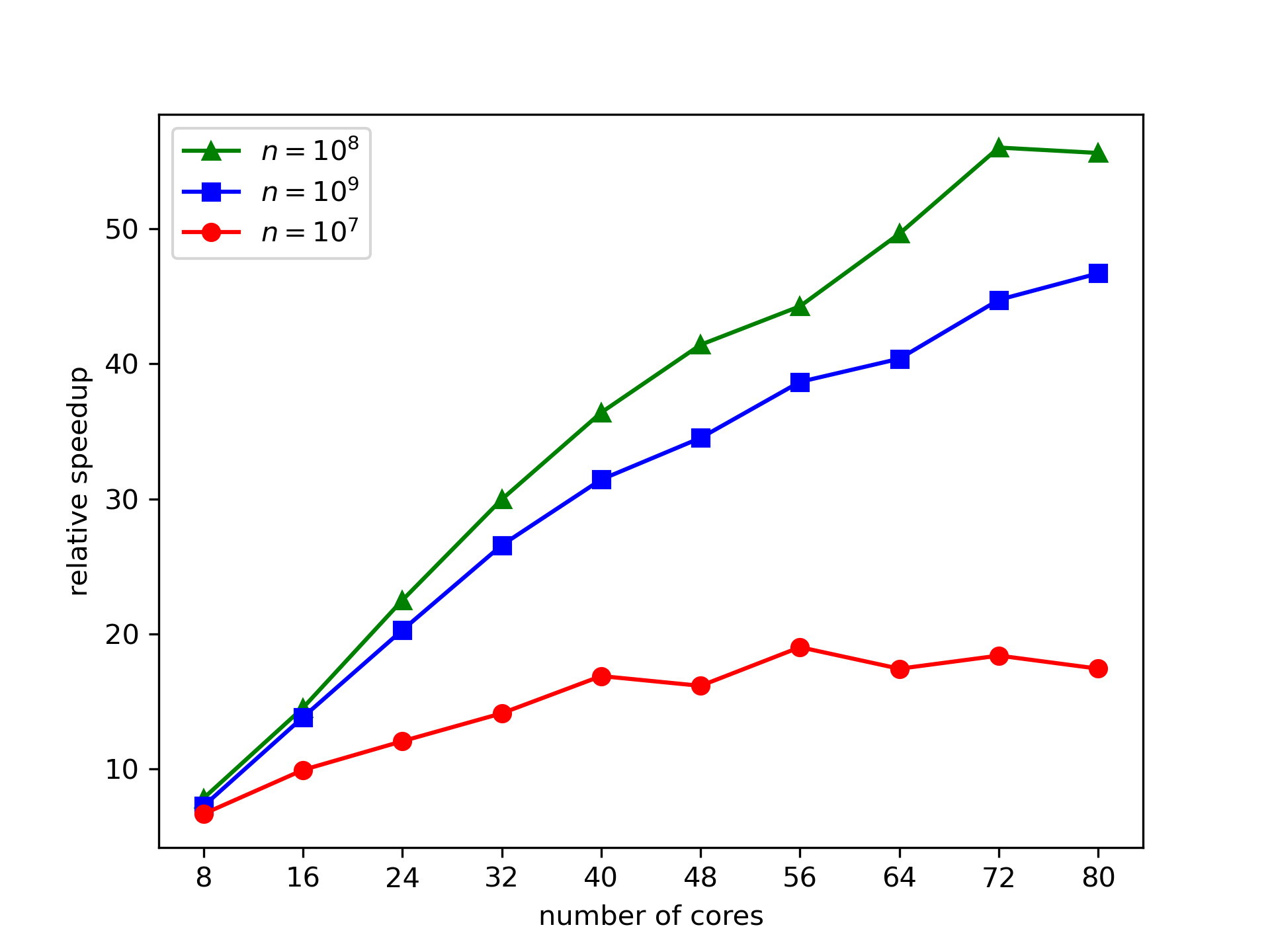
Instances in Figures 4 and 5 have varying input sizes of , with are drawn i.i.d. from . This demonstrates that the speedup per cores is a function of problem size. At , parallel Condat tails off in absolute speedup around 40 cores (where communication costs become marginally higher than overall gains), while consistently increasing speedups are observed up to 80 cores on the -sized instances. Similar patterns are observed for all algorithms in the relative speedups. For a fixed number of cores, larger instances yield larger partition sizes; hence the subvector projection problem given to each core tends to reduce more of the original vector, producing the observed effect for our parallel methods. More severe tailoff effects are observed in the Scan and Sort algorithms, which use an entirely different parallelization scheme.
For additional experiments varying , please see Appendix E.2.


5.1.2 ball
We conduct ball projection experiments with problem size . Inputs are drawn i.i.d. from . Algorithms were implemented as described in Sec 4.1. Results are shown in Figure 6. Similar to the standard projection onto Simplex problems, our parallel Condat implementation attains considerably superior results over the benchmark, with nearly 50X speedup.


5.1.3 Weighted Simplex and Weighted ball
We have conducted additional experiments using the weighted versions of simplex and ball projections. These have been placed in the online supplement, as results are similar. A description of the algorithms are given in Appendix B.2; pseudocode in Appendix D; and experimental results in Appendix E.3.
5.1.4 Parity Polytope
We conduct parity polytope projection experiments with a problem size setting of . Inputs are drawn i.i.d. from . Algorithms were implemented as described in Sec 4.2. Results are shown in Figure 7. Our parallel Condat has worse relative speedup on projections compared to parallel Michelot, but overall this still results in higher absolute speedups since the baseline serial Condat runs quickly. With up to around 20x absolute speedup in simplex projection subroutines from parallel Condat’s, we report an overall absolute speedup of up to around 2.75x for parity polytope projections. We note that the overall absolute speedup tails off more quickly; this is an expected effect from Amdahl’s law Amdahl (1967): diminishing returns due to partial parallelization of the algorithm.


5.1.5 Lasso on Real-World Data
We selected a dataset from a paper implementing a Lasso method (Wang et al. 2022): kdd2010 (named as kdda in the cited paper), and its updated version kdd2012; both of them can be found in LIBSVM data sets (Chang and Lin 2011). There are features in kdd2010 and features in kdd2012.
We implemented PGD with Mini-batch (Zhang et al. 2023, Sec. 12.5), and measure the runtime for subroutine of projecting onto ball, which is
where the initial point is drawn i.i.d. from sparse with sparse rate, with sample size and features, and includes labels for samples; moreover, . Moreover, we set samples in each iteration. We measure the runtime for ball projections for the first iterations. In later iterations the projected vector will be dense, at which point it is better to use serial projection methods (see Appendix E.5). Runtimes are measured by time_ns() Function), and the absolute speedup and relative speedup are reported in Figure 8 (for kdd2010) and Figure 9 (for kdd2012). Considerably more speedup is obtained for kdd2012, which may be due to problem size since the projection input vectors are more than twice the size of inputs from kdd2010.


5.1.6 Discussion
We observed consistent patterns of performance across a wide range of test instances, varying in size, distributions, and underlying projections. In terms of relative speedups, our parallelization scheme was surprisingly at least as effective as that of Sort and Scan. Parallel sort and parallel scan are well-studied problems in parallel computing, so we expected a priori for such speedups to be a strict upper bound on what our method could achieve. Thus our method is not simply benefiting from its compatibility with more advanced serial projection algorithms—the distributed method itself appears to be highly effective in practice.
6 Conclusion
We proposed a distributed preprocessing method for projection onto a simplex. Our method distributes subvector projection problems across processors in order to reduce the candidate index set on large-scale instances. One advantage of our method is that it is compatible with all major serial projection algorithms. Empirical results demonstrate, across a wide range of simulated distributions and real-world instances, that our parallelization of well-known serial algorithms are comparable and at times superior in relative speedups to highly developed and well-studied parallelization schemes for sorting and scanning. Moreover, the sort-and-scan serial approach involves substantially more work than e.g. Condat’s method; hence our parallelization scheme provides considerable absolute speedups in our experiments versus the state of the art.
The effectiveness depends on the sparsity of the projection; in the case of large-scale problems with i.i.d. inputs and , we can expect high levels of sparsity. A wide range of large-scale computational experiments demonstrates the consistent benefits of our method, which can be combined with any serial projection algorithms. Our experiments on real-world data suggest that significant sparsity can be exploited even when such distributional assumptions could be violated. We also note that, due to Proposition 2.1 and Corollary 2.2, highly dense projections occur when has a low value relative to the entries of . Now, iterative (serial) methods as Michelot’s and Condat’s can be interpreted as starting with a pivot value that is a lower bound on and increasing the pivot iteratively until the true value is attained. Hence, when our distributed method performs poorly due to density of the projection, the problem can simply be solved in serial using a small number of iterations, and vice-versa. This might be expected, for instance, when the input vector itself is sparse (see Appendix E.5).
7 Acknowledgements
This work was funded in part by the Office of Naval Research under grant N00014-23-1-2632. We also thank an anonymous reviewer for various code optimization suggestions.
References
- Amdahl (1967) Amdahl GM (1967) Validity of the single processor approach to achieving large scale computing capabilities. Proceedings of the April 18-20, 1967, spring joint computer conference, 483–485.
- Barlaud et al. (2017) Barlaud M, Belhajali W, Combettes PL, Fillatre L (2017) Classification and regression using an outer approximation projection-gradient method. IEEE Transactions on Signal Processing 65(17):4635–4644.
- Barman et al. (2013) Barman S, Liu X, Draper SC, Recht B (2013) Decomposition methods for large scale lp decoding. IEEE Transactions on Information Theory 59(12):7870–7886.
- Bentley and McIlroy (1993) Bentley JL, McIlroy MD (1993) Engineering a sort function. Software: Practice and Experience 23(11):1249–1256.
- Bioucas-Dias et al. (2012) Bioucas-Dias JM, Plaza A, Dobigeon N, Parente M, Du Q, Gader P, Chanussot J (2012) Hyperspectral unmixing overview: Geometrical, statistical, and sparse regression-based approaches. IEEE Journal of Selected Topics in Applied Earth Observations and Remote Sensing 5(2):354–379.
- Blondel et al. (2014) Blondel M, Fujino A, Ueda N (2014) Large-scale multiclass support vector machine training via euclidean projection onto the simplex. 2014 22nd International Conference on Pattern Recognition, 1289–1294.
- Blum et al. (1973) Blum M, Floyd RW, Pratt VR, Rivest RL, Tarjan RE, et al. (1973) Time bounds for selection. J. Comput. Syst. Sci. 7(4):448–461.
- Boyd and Vandenberghe (2004) Boyd S, Vandenberghe L (2004) Convex optimization (Cambridge University Press).
- Brodie et al. (2009) Brodie J, Daubechies I, De Mol C, Giannone D, Loris I (2009) Sparse and stable markowitz portfolios. Proceedings of the National Academy of Sciences 106(30):12267–12272.
- Candès et al. (2008) Candès EJ, Wakin MB, Boyd SP (2008) Enhancing sparsity by reweighted minimization. Journal of Fourier Analysis and Applications 14:877–905.
- Center (1987) Center OS (1987) Ohio supercomputer center. URL http://osc.edu/ark:/19495/f5s1ph73.
- Chang and Lin (2011) Chang CC, Lin CJ (2011) LIBSVM: A library for support vector machines. ACM Transactions on Intelligent Systems and Technology 2:27:1–27:27.
- Charles and J. Laurie (2006) Charles MG, J Laurie S (2006) Introduction to probability (American Mathematical Society).
- Chartrand and Yin (2008) Chartrand R, Yin W (2008) Iteratively reweighted algorithms for compressive sensing. 2008 IEEE International Conference on Acoustics, Speech and Signal Processing, 3869–3872.
- Chen et al. (1998) Chen SS, Donoho DL, Saunders MA (1998) Atomic decomposition by basis pursuit. SIAM Journal on Scientific Computing 20(1):33–61.
- Chen and Zhou (2014) Chen X, Zhou W (2014) Convergence of the reweighted minimization algorithm for - minimization. Computational Optimization and Applications 59:47–61.
- Cominetti et al. (2014) Cominetti, R M, WF S, PJS (2014) A newton’s method for the continuous quadratic knapsack problem. Math. Prog. Comp. 6:151––196.
- Condat (2016) Condat L (2016) Fast projection onto the simplex and the ball. Math. Program. Ser. A 158(1):575–585.
- Cormen et al. (2009) Cormen TH, Leiserson CE, Rivest RL, Stein C (2009) Introduction to Algorithms (The MIT Press), 3rd edition.
- Dai et al. (2006) Dai, YH F, R (2006) New algorithms for singly linearly constrained quadratic programs subject to lower and upper bounds. Math. Program. 106:403––421.
- Dai and Chen (2023) Dai Y, Chen C (2023) Sparsity-Exploiting Distributed Projections onto a Simplex. URL http://dx.doi.org/10.1287/ijoc.2022.0328.cd, https://github.com/INFORMSJoC/2022.0328.
- Donoho and Elad (2003) Donoho DL, Elad M (2003) Optimally sparse representation in general (nonorthogonal) dictionaries via l1 minimization. Proceedings of the National Academy of Sciences 100(5):2197–2202.
- Duchi et al. (2008) Duchi J, Shalev-Shwartz S, Singer Y, Chandra T (2008) Efficient projections onto the -ball for learning in high dimensions. Proceedings of the 25th International Conference on Machine learning (ICML), 272–279.
- Fischer (2011) Fischer H (2011) A history of the central limit theorem. From classical to modern probability theory (Springer).
- Gentle (2009) Gentle J (2009) Computational Statistics (Springer).
- Greb and Zachmann (2006) Greb A, Zachmann G (2006) Gpu-abisort: optimal parallel sorting on stream architectures. Proceedings 20th IEEE International Parallel & Distributed Processing Symposium, 10 pp.–.
- Held et al. (1974) Held M, Wolfe P, Crowder HP (1974) Validation of subgradient optimization. Math. Program. 6:62–88.
- Iutzeler and Condat (2018) Iutzeler F, Condat L (2018) Distributed projection on the simplex and ball via admm and gossip. IEEE Signal Processing Letters 25(11):1650–1654.
- Kiwiel (2008) Kiwiel KC (2008) Breakpoint searching algorithms for the continuous quadratic knapsack problem. Math. Program. 112:473–491.
- Knuth (1998) Knuth D (1998) The Art of Computer Programming, volume 1 (Addison-Wesley), 3rd edition.
- Ladner and Fischer (1980) Ladner RE, Fischer MJ (1980) Parallel prefix computation. J. ACM 27(4):831–838.
- Lagarias (2013) Lagarias JC (2013) Euler’s constant: Euler’s work and modern developments. Bull. Amer. Math. Soc. 50:527–628.
- Lellmann et al. (2009) Lellmann J, Kappes J, Yuan J, Becker F, Schnörr C (2009) Convex multi-class image labeling by simplex-constrained total variation. Scale Space and Variational Methods in Computer Vision, 150–162 (Springer Berlin Heidelberg).
- Liu and Draper (2016) Liu X, Draper SC (2016) The admm penalized decoder for ldpc codes. IEEE Transactions on Information Theory 62(6):2966–2984.
- Mahmoud (2000) Mahmoud HM (2000) Sorting: A distribution theory, volume 54 (John Wiley & Sons).
- Michelot (1986) Michelot C (1986) A finite algorithm for finding the projection of a point onto the canonical simplex of . Journal of Optimization Theory and Applications 50:195–200.
- Perez et al. (2020a) Perez G, Ament S, Gomes CP, Barlaud M (2020a) Efficient projection algorithms onto the weighted ball. CoRR abs/2009.02980.
- Perez et al. (2020b) Perez G, Michel Barlaud LF, Régin JC (2020b) A filtered bucket-clustering method for projection onto the simplex and the ball. Math. Program. Ser. A 182:445–464.
- Robinson et al. (1992) Robinson AG, Jiang N, Lerme CS (1992) On the continuous quadratic knapsack problem. Mathematical Programming 55:99–108.
- Tibshirani (1996) Tibshirani R (1996) Regression shrinkage and selection via the lasso. Journal of the Royal Statistical Society. Series B (Methodological) 58(1):267–288.
- Tibshirani (1997) Tibshirani R (1997) The lasso method for variable selection in the cox model. Statistic in Medicine 16:385–395.
- van den Berg (2020) van den Berg E (2020) A hybrid quasi-newton projected-gradient method with application to lasso and basis-pursuit denoising. Math. Program. Comp. 12:1–38.
- van den Berg and Friedlander (2009) van den Berg E, Friedlander MP (2009) Probing the pareto frontier for basis pursuit solutions. SIAM Journal on Scientific Computing 31(2):890–912.
- Wang et al. (2022) Wang G, Yu W, Liang X, Wu Y, Yu B (2022) An iterative reduction fista algorithm for large-scale lasso. SIAM Journal on Scientific Computing 44(4):A1989–A2017.
- Wang et al. (2020) Wang S, Bai Y, Pekhimenko G (2020) Bppsa: Scaling back-propagation by parallel scan algorithm.
- Wasson et al. (2019) Wasson M, Milicevic M, Draper SC, Gulak G (2019) Hardware-based linear program decoding with the alternating direction method of multipliers. IEEE Transactions on Signal Processing 67(19):4976–4991.
- Wei et al. (2015) Wei H, Jiao X, Mu J (2015) Reduced-complexity linear programming decoding based on admm for ldpc codes. IEEE Communications Letters 19(6):909–912.
- Xavier and Iyengar (1998) Xavier C, Iyengar SS (1998) Introduction to parallel algorithms, volume 1 (John Wiley & Sons).
- Zhang et al. (2023) Zhang A, Lipton ZC, Li M, Smola AJ (2023) Dive into deep learning.
- Zhang et al. (2013) Zhang G, Heusdens R, Kleijn WB (2013) Large scale lp decoding with low complexity. IEEE Communications Letters 17(11):2152–2155.
- Zhang and Siegel (2013) Zhang X, Siegel PH (2013) Efficient iterative lp decoding of ldpc codes with alternating direction method of multipliers. 2013 IEEE International Symposium on Information Theory, 1501–1505.
Appendix A Mathematical Proofs
Corollary 1 For any such that , we have
Proof.
By definition,
Observe that is a strictly decreasing function for , and for . Furthermore, from Proposition 1, we have that is the unique value such that ; moreover, since then . Thus , which implies , and . ∎
We assume uniformly distributed inputs, are , and we have
Lemma 1
with a sublinear convergence rate, where .
Proof.
Observe that . Since are i.i.d, then we have
| (7) |
Thus converges to sublinearly at the rate of
∎
Let denote the conditional variable such that .
We assume uniformly distributed inputs, are , and then
Proposition 2 Michelot’s method has an average runtime of .
Proof.
Let be the number of elements that Algorithm 3 (from the main body) removes from the (candidate) active set in iteration of the do-while loop, and let be the total number of iterations.
| (8) |
where is the active index set of the projection. Let be the th pivot (line 3 in Algorithm 3 of the main body) with
and define .
Now, from Proposition 9 we have that all with are i.i.d.. Thus , and so
| (9) |
In iteration , all elements in the range are removed, and again the i.i.d. uniform property is preserved by Proposition 9, so
by Law of Total Expectation,
Replacing the right-hand side expectation using Equation (9),
Using the Law of Total Expectation again,
| (10) |
Let . We will now consider cases. Observe that , i.e. the active set is a subset of the ground set. The following two cases exhaust the possibilities of where lies: either (Case 1); otherwise, either or (Case 2).
Case 1:
Let be an iteration such that satisfies:
Then,
| (11) |
Since , then from Michelot’s Method will stop within at most iterations since at least one element is removed in each iteration; thus . Since for ,
| (12) |
From Equation (10),
Then, from the Law of Total Expectation,
| (13) | ||||
Michelot’s method always maintains a nonempty active index set (decreasing per iteration), and so . Then, continuing from (13),
| (14) |
Claim.
.
Proof:
| (15) | ||||
Since and are ,
So for , since ,
| (16) |
Substituting into Inequality (15),
using Law of Total Expectation,
| (17) |
So then it remains to show . From Equation (9), for any iteration
thus, using the Law of Total Expectation,
| (18) |
Applying Equation (18) recursively, starting with the base case ,
Using the Law of Total Expectation,
From Inequality (16), ; thus
Since , ; thus ; as a result,
Thus . Substituting into Inequality (17)
The Claim, together with Inequality (14) establish that
Altogether with Inequalities (11) and (12), we have in Case 1.
Case 2: , or
If , let . Since
the Claim from Case 1 and Equation (14) hold for ; thus
If , then , which implies . However, are given independently of and so is fixed. Thus for asymptotic analysis, does not hold for sufficiently large .
Together with Case 1 and Case 2, . Hence operations are used for scanning/prefix-sum. All other operations, i.e. assigning and , are within a constant factor of the scanning operations. ∎
We assume uniformly distributed inputs, are , and we have
Lemma 2
Filter provides a pivot such that .
Proof.
The upper bound is given by construction of (see (Condat 2016, Section 3, Paragraph 2)).
We can establish the lower bound on by considering the sequence , which represents the initial as well as subsequent (intermediate) values of from the first outer for-loop on line 2 of presented as Algorithm 4 (from the main body), and their corresponding index sets . Filter initializes with and . For , if ,
otherwise , and . Then it can be shown that (see (Condat 2016, Section 3, Paragraph 2)), and (see (Condat 2016, Section 3, Paragraph 5)). Now in terms of we may write
For any , since then . By construction of and , we have . Thus, , and . So . ∎
Now we introduce some notation in order to compare subsequent iterations of Condat’s method with iterations of Michelot’s method. Let and be the total number of iterations taken by Condat’s method and Michelot’s method (respectively) on a given instance. Let be the active index sets per iteration for Condat’s method with corresponding pivots . Likewise, we denote the index sets and pivots of Michelot’s method as and , respectively. If then we set and ; likewise for Michelot’s algorithm.
Lemma 3
, and for .
Proof.
We will prove this by induction. For the base case, is obtained by Filter. So . Moreover, from Lemma 2, .
Now for any iteration , suppose , and . From line 5 in Algorithm 3 (from the main body), . From Condat (Condat 2016, Section 3, Paragraph 3), Condat’s method uses a dynamic pivot between to to remove inactive entries that would otherwise remain in Michelot’s method. Therefore, , and moreover for any , we have that . Now observe that
and so . ∎
Corollary 2 .
Proof.
Observe that both algorithms remove elements (without replacement) from their candidate active sets at every iteration; moreover, they terminate with the pivot value and so . So, together with Lemma 3, we have for that . So implies , and so . Therefore . ∎
Lemma 4 The worst-case runtime of Filter is .
Proof.
Since at any iteration, Filter will scan at most entries; including operations to update . ∎
We assume uniformly distributed inputs, are , and we have
Proposition 3
Condat’s method has an average runtime of .
Proof.
Filter takes operations from Lemma 4. From Corollary 2, the total operations spent on scanning in Condat’s method is less than (or equal to) the average operations for Michelot’s method (established in Proposition 2); hence Condat’s average runtime is . ∎
We assume uniformly distributed inputs, are , and we have
Theorem 1
.
Proof.
Lemma 5 Suppose are from an arbitrary distribution , with PDF and CDF . Let such that be some positive number, and be such that . Then i) as and ii) .
Proof.
Since is a density function, the CDF is absolutely continuous (see e.g. (Charles and J. Laurie 2006, Page 59, Definition 2.1)); thus for any , there exists such that .
For , define the indicator variable
and let . So , and we can show that it is binomially distributed.
Claim.
.
Proof: Observe that , and ; thus . Moreover, are independent, and so are i.i.d. ; consequently, .
So, as , we can apply the Central Limit Theorem (see e.g. Fischer (2011)):
| (21) |
Denote to be the CDF of the standard normal distribution. Consider (for any ) the right-tail probability
| (22) |
| (23) |
where is the floor function.
Setting yields
Consider the right-hand side, . Since is a CDF, it is monotonically increasing, continuous, and converges to ; thus . So as approaches infinity,
| (24) |
which establishes condition (i).
Now consider the left-tail probability,
Again setting , we have that . So as approaches infinity,
which establishes condition (ii). ∎
Theorem 2 Suppose are from an arbitrary distribution , with PDF and CDF . Then, for any , as .
Proof.
Case 1:
Since and , . Hence, .
Case 2:
Since is a density function, is absolutely continuous. So there exists be such that . We shall first establish that as .
From Corollary 1, , and so
| (25) |
Now observe that, for any , can be treated as a conditional variable: . Since all such are i.i.d, we may denote the (shared) expected value and variance as . Moreover, by definition of we have
| (26) |
Together with condition (i) of Lemma 5, this implies that the right-hand side of the probability in (25) is negative as :
| (27) |
It follows, continuing from Equation (25), that
Thus we have the desired result:
| (28) |
Now observe that implies , and subsequently . Together with condition (ii) from Lemma 5 we have
∎
Corollary 2 For projection of onto a simplex , if , the conclusion from Theorem 2 keeps true.
Proof.
Proposition 4 Let be a subvector of with entries; moreover, without loss of generality suppose the subvector contains the first entries. Let be the projection of onto the simplex , and be the corresponding pivot value. Then, . Consequently, for we have that .
Proof.
Define two index sets,
As is a subvector of , we have ; thus,
From Corollary 1, ; from Proposition 1 it thus follows that . ∎
We assume uniformly distributed inputs, are , and we have
Proposition 5
Parallel Pivot and Partition with either the median, random, or Michelot’s pivot rule, has an average runtime of .
Proof.
The algorithm starts by distributing projections. Pivot and Partition has linear runtime on average with any of the stated pivot rules, and so for the th core with input , whose size is , we have an average runtime of . Now from Theorem 1, each core returns in expectation at most active terms. So the reduced input (line 3 of Algorithm 8 from the main body) will have at most entries on average; thus the final projection will incur an expected number of operations in . ∎
We assume uniformly distributed inputs, are , and we have
Proposition 6
Let be the output of . Then .
Proof.
We assume that the if in line 5 from Algorithm 4 (from the main body) does not trigger; this is a conservative assumption as otherwise more elements would be removed from , reducing the number of iterations.
Let be the th pivot with (from line 1 in Algorithm 4 from the main body), and subsequent pivots corresponding to the for-loop iterations of line 2. Whenever Filter finds , it updates as follows:
| (29) |
Moreover, when is found, ; thus, from the Law of Total Expectation, . Together with (29),
Using the initial value , we can obtain a closed-form representation for the recursive formula:
| (30) |
Now let denote the number of terms Filter scans after calculating and before finding some . Since Filter scans terms in total (from initialize and calls to line 4), then
| (31) |
We can show has a geometric distribution as follows.
Claim.
.
Proof: For each term , we have
So can be interpreted as a Bernoulli trial. Hence is distributed with .
Now, applying Jensen’s Inequality to ,
and together with (30) we have
| (32) | ||||
Now observe that
where the first equality is from L’Hôpital’s rule. Thus . Furthermore, we have the classical bound on the harmonic series:
where is the Euler-Mascheroni constant, see e.g. Lagarias (2013); thus,
which implies . Moreover (see e.g. (Knuth 1998, Section 1.2.7)),
which implies . From (31) it follows that . ∎
We assume uniformly distributed inputs, are , and we have
Proposition 7
Parallel Condat’s method has an average complexity .
Proof.
In Distributed Filter (Algorithm 9 from the main body), each core is given input with . (serial) Filter has linear runtime from Lemma 4, and the for loop in line 5 of Algorithm 9 (from the main body) will scan at most terms. Thus distributed Filter runtime is in .
From Proposition 6, . Since the output of Distributed Filter is , we have that (given is i.i.d.) .
Parallel Condat’s method takes the input from Distributed Filter and applies serial Condat’s method (Algorithm 10 from the main body, lines 2-7), excluding the serial Filter. From Proposition 3, Condat’s method has average linear runtime, so this application of serial Condat’s method has average complexity . ∎
Lemma 6 If and , then .
Proof.
The CDF of is . Then,
which implies . ∎
Lemma 7 If are independent random variables, then are independent.
Proof.
are independent and so for any . So considering the joint conditional probability,
∎
Proposition 9 If i.i.d. and , then i.i.d. .
Proof.
From Lemma 6, for any , . From Lemma 7, for any , , are conditionally independent. So, i.i.d. . ∎
Appendix B Algorithm Descriptions
B.1 Bucket Method
Pivot and Partition selects one pivot in each iteration to partition and applies this recursively in order to create sub-partitions in the manner of a binary search. The Bucket Method, developed by Perez et al. (2020b), can be interpreted as a modification that uses multiple pivots and partitions (buckets) per iteration.
The algorithm, presented as Algorithm 11 is initialized with tuning parameters , the maximum number of iterations, and , the number of buckets with which to subdivide the data. In each iteration the algorithm partitions the problem into the buckets with the inner for loop of line 4, and then calculates corresponding pivot values in the inner for loop of line 10.
The tuning parameters can be determined as follows. Suppose we want the algorithm to find a (final) pivot within some absolute numerical tolerance of the true pivot , i.e. such that . This can be ensured (see Perez et al. (2020b)) by setting
where denotes the range of . Perez et al. Perez et al. (2020b) prove the worst-case complexity is .
We assume uniformly distributed inputs, are , and we have
Proposition 8
The Bucket method has an average runtime of .
Proof.
Let denote the index set at the start of iteration in the outer for loop (line 2), and denote the index set of the th bucket, , at the end of the first inner for loop (line 4).
For a given outer for loop iteration (line 2), the first inner for loop (line 4) uses operations. Note that the and on line 5 can be reused in each iteration, and the nested for loop on line 6 has iterations. The second inner for loop (line 10) also uses operations. In line 11, the first sum can be updated dynamically (in the manner of a scan) as a cumulative sum as is updated in line 16 or 19, thus requiring a constant number of operations per iteration . The second sum is bounded above by since . Thus each iteration of the outer for loop uses operations.
Since are i.i.d , then from Proposition 9, the terms from each sub-partition are also i.i.d uniform. So for any and , . From line 13, . Since then ; thus
Therefore, . ∎
B.2 Projection onto a Weighted Simplex and a Weighted Ball
The weighted simplex and the weighted ball are
where is a weight vector, and is a scaling factor. Perez et al. (2020a) show there is a unique such that , where . Thus pivot-based methods for the unweighted simplex extend to the weighted simplex in a straightforward manner. We present weighted Michelot’s method as Algorithm 3 (Appendix D), and weighted Filter as Algorithm 4 (Appendix D).
Our parallelization depends on the choice of serial method for projection onto simplex, since projection onto the weighted simplex requires direct modification rather than oracle calls to methods for the unweighted case. Sort and Scan for weighted simplex projection can be implemented with a parallel merge sort algorithm in Algorithm 5 (Appendix D). Our distributed structure can be applied to Michelot and Condat methods in a similar manner as with the unweighted case; these are presented respectively as Algorithms 6 and 7 (Appendix D). We note that projection onto is linear-time reducible to projection onto (Perez et al. 2020a, Equation (4)).
Appendix C Distribution Examples
Here we apply Theorem 2 to three examples:
(A) Let , , , .
(B) Let , , , .
(C) Let , , , .
Observe that
| (33a) | ||||
| (33b) | ||||
| (33c) | ||||
(33b) can be calculated by (28), and (33c) can be calculated by (23).
For (A), . From and , we have and . So,
Now, since , we have and . Applying Theorem 2 yields:
which implies the number of active elements in the projection should be less than of or with high probability.
For (B), ; similar to the first example,
Together with
we can calculate and :
Applying Theorem 2,
which imply of terms are active after projection with probability .
For (C), . Similar to the previous examples,
Together with
we can calculate and as follows,
Applying Theorem 2,
and so of terms are active after projection with probability .
Appendix D Algorithm Pseudocode
Appendix E Additional Experiments
All code and data can be found at: Github222https://github.com/foreverdyz/Parallel_Projection or the IJOC repository Dai and Chen (2023)
E.1 Testing Theoretical Bounds
For Theorem 1, we calculate the average number of active elements in projecting a vector , drawn i.i.d. from , onto the simplex , with between and and 10 trials per size. This empirical result is compared against the corresponding asymptotic bound of given by Theorem 1. Results are shown in Figure 10, and demonstrate that our asymptotic bound is rather accurate for small .
Similarly, for Proposition 6, we conduct the same experiments and compare the results against the function in Figure 11, where the constant was found empirically.
For Lemma 1, we run Algorithm 3 (in the main paper) on i.i.d. distributed inputs with scaling factor , size , and 100 trials. We compare the (average) remaining number of elements after each iteration of Michelot’s method and against the geometric series with a ratio as . We find the average number of remaining terms after each loop of Michelot’s method is close to the corresponding value of the geometric series with a ratio as from . So, the conclusion from Lemma 1, which claims that the Michelot method approximately discards half of the vector in each loop when the size is big, is accurate.


E.2 Robustness Test
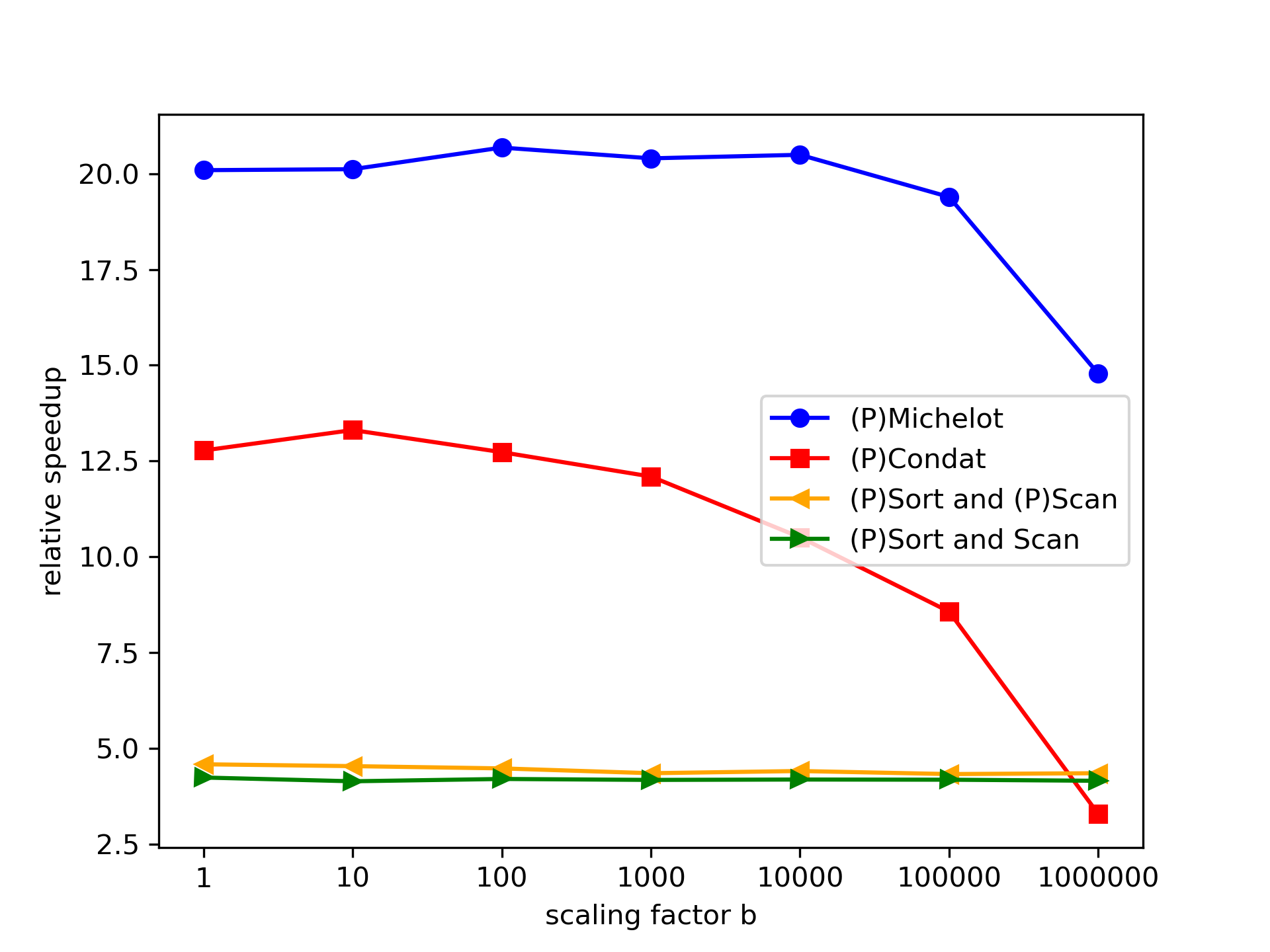
We created examples with a wide range of scaling factors , and drawing and with a size of for serial methods and parallel methods with cores. Results are given in Figure 13 () and Figure 14 ().


E.3 Weighted simplex, weighted ball
We conduct weighted simplex and weighted ball projection experiments with various methods to solve a problem with a problem size of . Inputs are drawn i.i.d. from and weights are drawn i.i.d. from . Algorithms were implemented as described in Sec B.2. Results for weighted simplex are shown in Figure 15 and results for weighted ball projection are shown in Fig. 16. Slightly more modest speedups across all algorithms are observed in the weighted simplex compared to the unweighted experiments; nonetheless, the general pattern still holds, with parallel Condat attaining superior performance with up to 14x absolute speedup. In the weighted ball projection, we observe that sort and scan has similar relative speedups to our parallel Condat’s method. However, the underlying serial Condat’s method is considerably faster.


E.4 Runtime Fairness Test
We provide a runtime fairness test for serial methods (e.g. Sort and Scan method, Michelot’s method, Condat’s method) and their respective parallel implements. We restrict both serail and parallel methods to use only one core to solve a problem with a size of and a scaling factor . Inputs drawn i.i.d. from , and . Results are provided in Table 3.
| Method | Runtime |
|---|---|
| Sort + Scan | |
| (P)Sort + Scan | |
| (P)Sort + Partial Scan | |
| Michelot | |
| (P) Michelot | |
| Condat | |
| (P) Condat |
E.5 Discussion on dense projections
To project a vector onto the ball, we first check if . If this condition holds, then is already within the ball. However, if , we project onto the simplex with a scaling factor of . As noted earlier, we have , which means that all zero terms in are inactive in the projection of onto the simplex. Therefore, we only need to project a subvector onto the simplex. This is why when is sparse, it is probably better to use serial projection methods instead of their parallel counterparts.