SparseBEV: High-Performance Sparse 3D Object Detection
from Multi-Camera Videos
Abstract
Camera-based 3D object detection in BEV (Bird’s Eye View) space has drawn great attention over the past few years. Dense detectors typically follow a two-stage pipeline by first constructing a dense BEV feature and then performing object detection in BEV space, which suffers from complex view transformations and high computation cost. On the other side, sparse detectors follow a query-based paradigm without explicit dense BEV feature construction, but achieve worse performance than the dense counterparts. In this paper, we find that the key to mitigate this performance gap is the adaptability of the detector in both BEV and image space. To achieve this goal, we propose SparseBEV, a fully sparse 3D object detector that outperforms the dense counterparts. SparseBEV contains three key designs, which are (1) scale-adaptive self attention to aggregate features with adaptive receptive field in BEV space, (2) adaptive spatio-temporal sampling to generate sampling locations under the guidance of queries, and (3) adaptive mixing to decode the sampled features with dynamic weights from the queries. On the test split of nuScenes, SparseBEV achieves the state-of-the-art performance of 67.5 NDS. On the val split, SparseBEV achieves 55.8 NDS while maintaining a real-time inference speed of 23.5 FPS. Code is available at https://github.com/MCG-NJU/SparseBEV.
1 Introduction
Camera-based 3D Object Detection [13, 54, 31, 11, 24, 25, 40] has witnessed great progress over the past few years. Compared with the LiDAR-based counterparts [19, 56, 4, 36], camera-based approaches have lower deployment cost and can detect long-range objects.

Previous methods can be divided into two paradigms. BEV (Bird’s Eye View)-based methods [13, 11, 25, 24, 40] follow a two-stage pipeline by first constructing an explicit dense BEV feature from multi-view features and then performing object detection in BEV space. Although achieving remarkable progress, they suffer from high computation cost and rely on complex view transformation operators. Another line of work [54, 31, 32] explores the sparse query-based paradigm by initializing a set of sparse reference points in 3D space. Specifically, DETR3D [54] links the queries to image features using 3D-to-2D projection. It has simpler structure and faster speed, but its performance still lags far behind the dense ones. PETR series [31, 32] uses dense global attention for the interaction between query and image feature, which is computationally expensive and buries the advantage of the sparse paradigm. Thus, a natural question arises whether fully sparse detectors achieve similar accuracy to the dense ones?
In this paper, we find that the key to obtain high performance in sparse 3D object detection is the adaptability of the detector in both BEV and image space. In BEV space, the detector should be able to aggregate multi-scale features adaptively. Dense BEV-based detectors typically use a BEV encoder to encode multi-scale BEV features. It can be a stack of residual blocks with FPN [26] (e.g. BEVDet [26]), or a transformer encoder with multi-scale deformable attention [60] (e.g. BEVFormer [25]). For sparse detectors such as DETR3D, we argue that the multi-head self attention (MHSA) [49] among queries can play the role of the BEV encoder, as queries are defined in BEV space. However, the vanilla MHSA has a global receptive field, lacking an explicit multi-scale design. In image space, the detector should be adaptive to different objects with different sizes and categories. This is because although the objects have similar sizes in 3D space, they might vary greatly in images. However, the single-point sampling in DETR3D has a fixed local receptive field and the sampled feature is processed by static linear layers, hindering its performance.
To this end, we present SparseBEV, a fully sparse 3D object detector that matches or even outperforms the dense counterparts. Our SparseBEV detector contains three key designs, which are (1) scale-adaptive self attention to aggregate features with adaptive receptive field in BEV space, (2) adaptive spatio-temporal sampling to generate sampling locations under the guidance of queries, and (3) adaptive mixing to decode the sampled features with dynamic weights from the queries. We also propose to use pillars instead of reference points as the formulation of query, since pillars introduce better spatial priors.
We conduct comprehensive experiments on the nuScenes dataset. As shown in Fig. 1, our SparseBEV achieves the performance of 55.8 NDS and the speed of 23.5 FPS on the val split, surpassing all previous methods in both speed and accuracy. Besides, we can flexibly adjust of the inference speed by reducing the number of decoder layers without re-training. On test split, SparseBEV with V2-99 [20] backbone achieves 63.6 NDS without using future frames or test-time augmentation. By further utilizing future frames, SparseBEV achieves 67.5 NDS, outperforming the previous state-of-the-art BEVFormerV2 [55] by 2.7 NDS.
2 Related Work
2.1 Query-based 2D Object Detection
Recently, Transformer [49] with its attention blocks has been widely applied in the computer vision tasks [5, 8, 2]. In object detection, DETR [2] was the first model to predict objects based on learnable queries and treat the detection as a set prediction problem. A lot of works [60, 45, 30, 37, 7, 21, 57] were then proposed to accelerate the convergence of DETR by using the sampled features instead of using the global ones. For example, Deformable-DETR [60] samples image features based on sparse reference points, and then applies the deformable attention on the features. Sparse R-CNN [45] uses the ROIAlign [9] to obtain local features and then performs the dynamic convolution. AdaMixer [7] combines the advantages of the sampling points and the dynamic convolution to further boost the convergence. DN-DETR [21] devises a denoising mechanism that feeds ground-truth bounding boxes with noises into decoder and trains the model to reconstruct the original boxes. DINO [57] furtherly optimizes DN-DETR [21] and DAB-DETR [30] by proposing a contrastive denoising training strategy and a mixed query selection method. There are also several methods [3, 14, 46] designed to tackle the instability of the training procedure. Our work follows the query-based detection paradigm and extends it to 3D space with temporal information.
2.2 Monocular 3D Object Detection
Monocular 3D object detection takes one single image as input and outputs predicted 3D bounding boxes of objects. A significant challenge in monocular 3D object detection is how to transfer 2D features to 3D space. Several works [53, 43, 51, 39] incorporates depth information to deal with this problem. Pseudo LiDAR [53] first estimates the depth of input images and constructs pseudo point clouds. The pseudo point clouds are then sent to a LiDAR-based detection module to predict the 3D boxes of interested objects. CaDDN [43] further proposes a fully differentiable end-to-end network which learns pixel-wise categorical depth distributions to predict appropriate depth intervals in 3D space. Inspired by FCOS [47], FCOS3D [51] projects 3D coordinates onto 2D images and decouples them as 2D attributes (centerness and classification) and 3D attributes (depths, sizes, and orientations).
2.3 3D Object Detection in BEV

Bird’s-eye-view (BEV) object detection [38, 42, 13, 54, 31, 58, 25, 55, 40] aims at detecting objects in BEV space given either single-view or multi-view 2D images. Early works [44, 53, 43] typically transformed 2D features to BEV space based on single-view images and conducted monocular 3D object detection. LSS [42] takes six 2D images of different views as input and transforms them into 3D space based on depth estimation. Based on LSS, BEVDet [13] lifts 2D feature to BEV space and uses a BEV encoder with residual blocks and FPN to further encode the BEV features. BEVFormer [25] proposes a spatio-temporal transformer encoder that projects multi-view and multi-timestamp input to BEV representations. To ease the optimization, BEVFormerV2 [55] introduces perspective view supervision and supervises monocular 3D object detection parallel with BEV object detection. SOLOFusion [40] defines the localization potential for depth estimation and fuses short-term, high-resolution and long-term, low-resolution temporal stereo.
Inspired by DETR, another line of works [54, 31, 32] explore the sparse query-based paradigm. DETR3D [54] proposes a top-down framework starting from a learnable sparse set of reference points and refining them iteratively via 3D-to-2D queries. However, such 3D-to-2D projection hinders the receptive field of the query. To handle this, PETR series [31, 32] use global attention for the interaction betweeen queries and image features, and introduce 3D positional embeddings to encode 2D features into 3D representation without explicit projection. Although achieving notable improvements, the expensive dense global attention buries the advantages of the sparse paradigm and makes it difficult to utilize long-term temporal information efficiently. In contrast, we keep the fully sparse design of DETR3D and boost the performance by enhancing the adaptability of the detector.
3 SparseBEV
As shown in Fig. 2, SparseBEV is a query-based one-stage detector with decoder layers. The input multi-camera videos are processed frame-by-frame using image backbone and FPN. Next, a set of sparse pillar queries are initialized in BEV space and aggregated by scale-adaptive self attention. These queries then interact with the image features via adaptive spatio-temporal sampling and adaptive mixing to make 3D object predictions. We also propose a dual-branch version of SparseBEV to further enhance the temporal modeling.
3.1 Query Formulation
We first define a set of learnable queries, where each of them is represented by its translation , dimension , rotation and velocity . The queries are initialized to be pillars in BEV space where is set to 0 and is set to 4m. The initial velocity is set to . Other parameters () are drawn from random gaussian distributions. Following Sparse R-CNN[45], we attach a -dim query feature to each query box to encode the rich instance characteristics.
3.2 Scale-adaptive Self Attention
As mentioned above, dense BEV-based methods typically use a BEV encoder to encode multi-scale BEV features. However, in our method, since we do not explicitly build a BEV feature, how to aggregate multi-scale features in BEV space is a challenge.
In this work, we argue that the self attention can play the role of BEV encoder, since queries are defined in BEV space. The vanilla multi-head self attention has global receptive field and lacks the ability of local multi-scale aggregation. Thus, we propose scale-adaptive self attention (SASA), which learns appropriate receptive fields under the guidance of queries. First, we compute the all-pair distances ( is the number of queries) between the query centers in BEV space:
| (1) |
where and denotes the center of the -th query. The attention considers not only the similarity between query features, but the distance between them as well. A toy example below shows how it works:
| (2) |
where is the query itself and is the channel dimension. is a scalar to control the receptive field for each query. When , it degrades to the vanilla self attention with global receptive field. As grows, the attention weights for distant queries becomes smaller and the receptive field narrows.
In practice, the receptive field controller is adaptive to each query and specific to each head. Supposing there are heads, we use a linear transformation to generate head-specific from the give query :
| (3) |
where the weights are shared across different queries.


In our experiments, we surprisingly find that the for each head is learnt to uniformly distribute in a certain range regardless of the initialization. In Fig. 3, we sort the heads according to and visualize the attention weights for the distance part. As we can see, each head learns a different receptive field from each other, enabling the network to aggregate features in a multi-scale manner like FPN.
Scale-adaptive self attention (SASA) demonstrates the necessity of FPN, while being more flexible as it learns the scales adaptively from the query. We also find an interesting phenomenon that different categories of queries have different sizes of receptive field. For example, queries representing the bus have larger receptive field than those representing the pedestrians. More details can be found in the ablation studies.
3.3 Adaptive Spatio-temporal Sampling
For each frame, we use a linear layer to generate a set of sampling offsets adaptively from the query feature. These offsets are transformed to 3D sampling points based on the query pillar:
| (16) |
Compared with the deformable attention in BEVFormer, our sampling points are adaptive to both query pillar and query feature, thus better covering objects with varying sizes. Besides, these points are not restricted to the query, since we do not limit the range of the sampling offsets.
Next, we perform temporal alignment by warping the sampling points according to motions. In autonomous driving, there are two types of motion: one is ego-motion and the other is object motion. Ego-motion describes the motion of the car from its own perspective as it navigates through the environment, while object motion refers to the movement of other objects in the environment as they move around the self-driving car.
Dealing with Object Motion.
As mentioned above, instantaneous velocity can be equal to average velocity for a short time window in self-driving. Thus, we adaptively warp the sampling points to previous timestamps using the velocity vector from the query:
| (17) | ||||
| (18) |
where denotes the timestamp of previous frame ( denotes the current timestamp). Note that is identical to because the velocity vector is defined in BEV plane.
Dealing with Ego Motion.
Next, we warp the sampling points based on the ego pose provided by the dataset. Points are first transformed to the global coordinate system and then to the local coordinate system of frame :
| (19) |
where is the ego pose of frame .
| Method | Backbone | Input Size | Epochs | NDS | mAP | mATE | mASE | mAOE | mAVE | mAAE |
|---|---|---|---|---|---|---|---|---|---|---|
| PETRv2 [32] | ResNet50 | 704 256 | 60 | 45.6 | 34.9 | 0.700 | 0.275 | 0.580 | 0.437 | 0.187 |
| BEVStereo [22] | ResNet50 | 704 256 | 90 | 50.0 | 37.2 | 0.598 | 0.270 | 0.438 | 0.367 | 0.190 |
| BEVPoolv2 [12] | ResNet50 | 704 256 | 90 | 52.6 | 40.6 | 0.572 | 0.275 | 0.463 | 0.275 | 0.188 |
| SOLOFusion [40] | ResNet50 | 704 256 | 90 | 53.4 | 42.7 | 0.567 | 0.274 | 0.511 | 0.252 | 0.181 |
| Sparse4Dv2 [29] | ResNet50 | 704 256 | 100 | 53.9 | 43.9 | 0.598 | 0.270 | 0.475 | 0.282 | 0.179 |
| StreamPETR [50] | ResNet50 | 704 256 | 60 | 55.0 | 45.0 | 0.613 | 0.267 | 0.413 | 0.265 | 0.196 |
| SparseBEV | ResNet50 | 704 256 | 36 | 54.5 | 43.2 | 0.606 | 0.274 | 0.387 | 0.251 | 0.186 |
| SparseBEV | ResNet50 | 704 256 | 36 | 55.8 | 44.8 | 0.581 | 0.271 | 0.373 | 0.247 | 0.190 |
| DETR3D [54] | ResNet101-DCN | 1600 900 | 24 | 43.4 | 34.9 | 0.716 | 0.268 | 0.379 | 0.842 | 0.200 |
| BEVFormer [25] | ResNet101-DCN | 1600 900 | 24 | 51.7 | 41.6 | 0.673 | 0.274 | 0.372 | 0.394 | 0.198 |
| BEVDepth [24] | ResNet101 | 1408 512 | 90 | 53.5 | 41.2 | 0.565 | 0.266 | 0.358 | 0.331 | 0.190 |
| Sparse4D [28] | ResNet101-DCN | 1600 900 | 48 | 55.0 | 44.4 | 0.603 | 0.276 | 0.360 | 0.309 | 0.178 |
| SOLOFusion [40] | ResNet101 | 1408 512 | 90 | 58.2 | 48.3 | 0.503 | 0.264 | 0.381 | 0.246 | 0.207 |
| SparseBEV | ResNet101 | 1408 512 | 24 | 59.2 | 50.1 | 0.562 | 0.265 | 0.321 | 0.243 | 0.195 |
Sampling.
For each timestamp, we project the warped sampling points to each view using the provided camera intrinsics and extrinsics. Since there are overlaps between adjacent views, the projected point may hit one or more views, which are termed as . For each hit view , we have multi-scale feature maps from the image backbone. Features are first sampled by bilinear interpolation in the image plane and then weighted over the scale axis:
| (20) |
where is the number of the multi-scale feature maps and is the projection function for view . is the weight for the -th point on the -th feature map and is generated from the query feature by linear transformation.
3.4 Adaptive Mixing
Given the sampled features from different timestamps and locations, the key is how to adaptively decode it under the guidance of queries. Inspired by AdaMixer [7], we introduce a simple but effective approach to decode and aggregate the spatio-temporal features with dynamic convolutions [15] and MLP-Mixer [48]. Supposing there are frames in total and sampling points per frame, we first stack them to a total of points. Thus, the sampled features are organized to .
Channel Mixing.
We first perform channel mixing on to enhance object semantics. The dynamic weights are generated from the query feature :
| (21) | ||||
| (22) |
where is the dynamic weights and is shared across different frames and different sampling points.
Point Mixing.
Next, we then transpose the feature and apply the dynamic weights to the point dimension of it:
| (23) | ||||
| (24) |
where is the dynamic weights and is shared across different channels.
After channel mixing and point mixing, the spatio-temporal features are flattened and aggregated by a linear layer. The final regression and classification predictions are computed by two MLPs respectively.
| Method | Backbone | Epochs | NDS | mAP | mATE | mASE | mAOE | mAVE | mAAE |
| DETR3D [54] | V2-99 | 24 | 47.9 | 41.2 | 0.641 | 0.255 | 0.394 | 0.845 | 0.133 |
| PETR [31] | V2-99 | 24 | 50.4 | 44.1 | 0.593 | 0.249 | 0.383 | 0.808 | 0.132 |
| UVTR [23] | V2-99 | 24 | 55.1 | 47.2 | 0.577 | 0.253 | 0.391 | 0.508 | 0.123 |
| BEVFormer [25] | V2-99 | 24 | 56.9 | 48.1 | 0.582 | 0.256 | 0.375 | 0.378 | 0.126 |
| BEVDet4D [11] | Swin-B [33] | 90‡ | 56.9 | 45.1 | 0.511 | 0.241 | 0.386 | 0.301 | 0.121 |
| PolarFormer [16] | V2-99 | 24 | 57.2 | 49.3 | 0.556 | 0.256 | 0.364 | 0.440 | 0.127 |
| PETRv2 [32] | V2-99 | 24 | 59.1 | 50.8 | 0.543 | 0.241 | 0.360 | 0.367 | 0.118 |
| Sparse4D [28] | V2-99 | 48 | 59.5 | 51.1 | 0.533 | 0.263 | 0.369 | 0.317 | 0.124 |
| BEVDepth [24] | V2-99 | 90‡ | 60.0 | 50.3 | 0.445 | 0.245 | 0.378 | 0.320 | 0.126 |
| BEVStereo [22] | V2-99 | 90‡ | 61.0 | 52.5 | 0.431 | 0.246 | 0.358 | 0.357 | 0.138 |
| SOLOFusion [40] | ConvNeXt-B [34] | 90‡ | 61.9 | 54.0 | 0.453 | 0.257 | 0.376 | 0.276 | 0.148 |
| SparseBEV | V2-99 | 24 | 62.7 | 54.3 | 0.502 | 0.244 | 0.324 | 0.251 | 0.126 |
| SparseBEV (dual-branch) | V2-99 | 24 | 63.6 | 55.6 | 0.485 | 0.244 | 0.332 | 0.246 | 0.117 |
| BEVFormerV2 [55] | InternImage-XL [52] | 24 | 64.8 | 58.0 | 0.448 | 0.262 | 0.342 | 0.238 | 0.128 |
| BEVDet-Gamma [12] | Swin-B | 90‡ | 66.4 | 58.6 | 0.375 | 0.243 | 0.377 | 0.174 | 0.123 |
| SparseBEV | V2-99 | 24 | 67.5 | 60.3 | 0.425 | 0.239 | 0.311 | 0.172 | 0.116 |
3.5 Dual-branch SparseBEV
Inspired by SlowFast [6], we further enhance the long-term temporal modeling by dividing the input video into a slow stream and a fast stream, resulting in a dual-branch SparseBEV. The slow stream is designed to capture fine-grained appearance details and it operates at low frame rates and high resolutions. The fast stream is responsible for capturing long-term temporal stereo and it operates at high frame rates and low resolutions. Sampling points are projected to the two streams respectively and the sampled features are stacked before adaptive mixing.
In this way, we decouple the learning of static appearance and temporal motion, leading to better performance. Besides, the computation cost is significantly reduced since only a small fraction of frames needs to be processed at high resolution. However, since this dual-branch design makes the framework a little complex, we do not use it unless otherwise stated. The ablations of this part can be found in the supplementary material.
4 Experiments
4.1 Implementation Details
We implement our model using PyTorch [41]. Following previous methods [54, 25, 32, 40], we adopt common image backbones including ResNet [10] and V2-99 [20]. The decoder consists of 6 layers and weights are shared across different layers. By default, we use frames in total and the interval between adjacent frames is about 0.5s.
During training, we adopt the Hungarian algorithm [18] for label assignment between ground-truth objects and predictions. Focal loss [27] is used for classification and L1 loss is used for 3D bounding box regression. We use the AdamW [35] optimizer with a global batch size of 8. The initial learning rate is set to and is decayed with cosine annealing policy.
Recently, we follow the training setting of the very recent work StreamPETR [50] and refresh our results for fair comparison. For the regression loss, we change the loss weight of and to 2.0 and leave the others to 1.0. Query denoising [21] is also introduced to stablize training and speedup convergence.
4.2 Datasets and Metrics
We evaluate our model on the nuScenes dataset [1], which consists of large-scale multimodal data collected from 6 surround-view cameras, 1 lidar and 5 radars. The dataset has 1000 videos and is split into 700/150/150 videos for training/validation/testing. Each video has roughly 20s duration and the key samples are annotated every 0.5s.
For 3D object detection, there are up to 1.4M annotated 3D bounding boxes of 10 classes. The official evaluation metrics include the well-known mean Average Precision (mAP) and five true positive (TP) metrics, including ATE, ASE, AOE, AVE, and AAE for measuring translation, scale, orientation, velocity, and attribute errors respectively. The overall performance is measured by the nuScenes Detection Score (NDS), which is the composite of the above metrics.
4.3 Comparison with the State-of-the-art Methods
nuScenes val split.
In Tab. 1, we compare SparseBEV with previous state-of-the-art methods on the validation split of nuScenes. Unless otherwise stated, the image backbone is pretrained on ImageNet-1k [17] and the number of queries is set to 900. To keep the simplicity of our approach, the dual-branch design is not used here. When adopting ResNet50 as the backbone and 704 256 as the input size, SparseBEV outperforms the previous state-of-the-art method SOLOFusion by 1.1 NDS and 0.5 mAP. By further adopting nuImages [1] pretraining and reducing the number queries to 400, SparseBEV sets a new record of 55.8 NDS while maintaining a real-time inference speed of 23.5 FPS (corresponding to Fig. 1). Next, we upgrade the backbone to ResNet101 and scale the input size up to 1408 512. Under this setting, SparseBEV still surpasses SOLOFusion by 1.8 mAP and 1.0 NDS, demonstrating the scalability of our method.
nuScenes test split.
We submit our method to the website of nuScenes and report the leaderboard in Tab. 2. Using the V2-99 [20] backbone pretrained by DD3D [39], SparseBEV achieves 62.7 NDS and 54.3 mAP without bells and whistles. Built on top of this, the dual-branch design gives us extra bonus on the performance, hitting 63.6 NDS and 55.6 mAP. We also follow the offline setting of BEVFormerV2 [55] which leverages both past and future frames to assist the detection. Remarkably, our method (single branch only) surpasses BEVFormerV2 by 2.8 mAP and 2.2 NDS. In addition, BEVFormerV2 uses InternImage-XL [52] with over 300M parameters as the image backbone, while our V2-99 backbone is much more lightweight with only 70M parameters.
4.4 Ablation Studies
In this section, we conduct ablations on the validation split of nuScenes. For all experiments, we use ResNet50 pretrained on nuImages [1] as the image backbone. The input contains 8 frames with 704 256 resolution. We use 900 queries in the decoder and the model is trained for 24 epochs without CBGS [59].
| Query Formulation | NDS | mAP |
|---|---|---|
| 3D Reference Points | 55.1 | 44.0 |
| BEV Pillars | 55.6 | 45.4 |
Query Formulation.
In Tab. 3, we ablate different formulations of the query. The top row uses a set of reference points distributing uniformly in 3D space (e.g. DETR3D and PETR). By replacing the reference points with pillars in BEV space, we observe performance improvements (+0.5 NDS) over the baseline. This is because pillars introduce better spatial priors than reference points.
| Self Attention | Distance Function | NDS | mAP |
|---|---|---|---|
| MHSA | - | 53.4 | 41.4 |
| SASA | 54.3 | 43.8 | |
| 55.6 | 45.4 | ||
| 55.1 | 44.3 |

Scale-adaptive Self Attention.
We study the effect of scale-adaptive self attention (SASA) in Tab. 4. Compared with the vanilla multi-head self attention, SASA achieves +4.0 mAP and +2.2 NDS improvements over the baseline. We further ablate different distance functions and find that distance works best. Besides, we also observe two interesting phenomena in SASA. First, different heads learn a different receptive field (see Fig. 3), enabling the model to aggregate multi-scale features in BEV space. Second, queries representing larger objects tend to have larger receptive field. In Fig. 4, we average the receptive field coefficient over all queries and all heads for each class. As we can see, the receptive field of large objects (such as bus and truck) is larger than small objects (such as pedestrian and traffic cone), demonstrating the effectiveness of our adaptive design.


Adaptive Spatio-temporal Sampling.
In Fig. 5, we ablate the number of frames and sampling points. The performance continues to improve as the number of frames increases, proving that SparseBEV can benefit from the long-term history. Here, we use 8 frames for fair comparison with previous methods. As for the number of sampling points, we observe that dispatching 16 points for each frame leads to the best performance. We also provide the visualization of the sampling points from the last stage of the decoder in Fig. 6. Our sampling scheme has adaptive regions of interest and achieves good temporal alignments for both static and moving objects across different frames.
| Ego Align | Obj. Align | NDS | mAP | mAVE |
|---|---|---|---|---|
| - | - | 44.4 | 34.1 | 0.510 |
| - | 54.2 | 43.5 | 0.281 | |
| 55.6 | 45.4 | 0.243 |
Temporal Alignment.
In Tab. 5, we validate the necessity of temporal alignment in spatio-temporal sampling. In our method, ego motion is aligned with the provided ego pose, while object motion is aligned with a simple constant velocity motion model. As we can see from the table, both of them contribute to the performance.
Adaptive Mixing.
In Tab. 6, we validate the design of the adaptive mixing. The top row is a baseline that uses attention weights to aggregate sampled features (as done in DETR3D). Static mixing and adaptive mixing improve the baseline by 2.7 NDS and 6.5 NDS respectively, demonstrating the necessity of the adaptive design. Next, we explore different combinations of channel and point mixing. Channel mixing followed by point mixing leads to better performance, proving that the object semantics should be enhanced before point mixing.
4.5 Limitations and Future Work
One limitation of SparseBEV is the heavy reliance on ego pose. As we can see from Tab. 5, the performance drops about 10 NDS without ego-based temporal alignment. However, in the real world, the ego pose provided by IMU may be unreliable and inaccurate, seriously affecting the robustness. Another limitation is that the inference latency increases linearly with the number of frames, since we stack the sampled features along the temporal dimension.
In the future, we will explore a more elegant and concise way of decoupling spatial appearance and temporal motion. We will also try to extend SparseBEV to other 3D perception tasks such as BEV segmentation, occupancy prediction and lane detection.
| Method | Details | NDS | mAP |
|---|---|---|---|
| W/o Mixing | - | 49.1 | 38.6 |
| Static Mixing | Channel Point | 51.8 | 41.9 |
| Adaptive Mixing | Channel Only | 53.1 | 42.7 |
| Point Only | 53.6 | 43.3 | |
| Point Channel | 55.4 | 44.6 | |
| Channel Point | 55.6 | 45.4 |
5 Conclusion
In this paper, we have proposed a query-based one-stage 3D object detector, named SparseBEV, which can enjoy the benefits of the BEV space without explicitly constructing a dense BEV feature. SparseBEV improves the adaptability of the decoder by three key modules: scale-adaptive self attention, adaptive spatio-temporal sampling and adaptive mixing. We further introduce a dual-branch design to enhance the long-term temporal modeling. Experiments show that SparseBEV achieves the state-of-the-art performance on the dataset of nuScenes for both speed and accuracy. We hope this exciting result will attract more attention to the fully sparse BEV detection paradigm.
Acknowledgements.
This work is supported by National Key RD Program of China (No. 2022ZD0160900), National Natural Science Foundation of China (No. 62076119, No. 61921006), Fundamental Research Funds for the Central Universities (No. 020214380091, No. 020214380099), and Collaborative Innovation Center of Novel Software Technology and Industrialization. Besides, the authors would like to thank Ziteng Gao, Zhiqi Li and Ruopeng Gao for their help.
References
- [1] Holger Caesar, Varun Bankiti, Alex H Lang, Sourabh Vora, Venice Erin Liong, Qiang Xu, Anush Krishnan, Yu Pan, Giancarlo Baldan, and Oscar Beijbom. nuscenes: A multimodal dataset for autonomous driving. In Proceedings of the IEEE/CVF conference on computer vision and pattern recognition, pages 11621–11631, 2020.
- [2] Nicolas Carion, Francisco Massa, Gabriel Synnaeve, Nicolas Usunier, Alexander Kirillov, and Sergey Zagoruyko. End-to-end object detection with transformers. In Proceedings of the European conference on computer vision, pages 213–229, 2020.
- [3] Qiang Chen, Xiaokang Chen, Gang Zeng, and Jingdong Wang. Group detr: Fast training convergence with decoupled one-to-many label assignment. arXiv preprint arXiv:2207.13085, 2022.
- [4] Yukang Chen, Jianhui Liu, Xiaojuan Qi, Xiangyu Zhang, Jian Sun, and Jiaya Jia. Scaling up kernels in 3d cnns. arXiv preprint arXiv:2206.10555, 2022.
- [5] Alexey Dosovitskiy, Lucas Beyer, Alexander Kolesnikov, Dirk Weissenborn, Xiaohua Zhai, Thomas Unterthiner, Mostafa Dehghani, Matthias Minderer, Georg Heigold, Sylvain Gelly, et al. An image is worth 16x16 words: Transformers for image recognition at scale. arXiv preprint arXiv:2010.11929, 2020.
- [6] Christoph Feichtenhofer, Haoqi Fan, Jitendra Malik, and Kaiming He. Slowfast networks for video recognition. In Proceedings of the IEEE/CVF international conference on computer vision, pages 6202–6211, 2019.
- [7] Ziteng Gao, Limin Wang, Bing Han, and Sheng Guo. Adamixer: A fast-converging query-based object detector. In Proceedings of the IEEE/CVF Conference on Computer Vision and Pattern Recognition, pages 5364–5373, 2022.
- [8] Meng-Hao Guo, Cheng-Ze Lu, Qibin Hou, Zhengning Liu, Ming-Ming Cheng, and Shi-Min Hu. Segnext: Rethinking convolutional attention design for semantic segmentation. arXiv preprint arXiv:2209.08575, 2022.
- [9] Kaiming He, Georgia Gkioxari, Piotr Dollár, and Ross Girshick. Mask r-cnn. In Proceedings of the IEEE international conference on computer vision, pages 2961–2969, 2017.
- [10] Kaiming He, Xiangyu Zhang, Shaoqing Ren, and Jian Sun. Deep residual learning for image recognition. In Proceedings of the IEEE conference on computer vision and pattern recognition, pages 770–778, 2016.
- [11] Junjie Huang and Guan Huang. Bevdet4d: Exploit temporal cues in multi-camera 3d object detection. arXiv preprint arXiv:2203.17054, 2022.
- [12] Junjie Huang and Guan Huang. Bevpoolv2: A cutting-edge implementation of bevdet toward deployment. arXiv preprint arXiv:2211.17111, 2022.
- [13] Junjie Huang, Guan Huang, Zheng Zhu, and Dalong Du. Bevdet: High-performance multi-camera 3d object detection in bird-eye-view. arXiv preprint arXiv:2112.11790, 2021.
- [14] Ding Jia, Yuhui Yuan, Haodi He, Xiaopei Wu, Haojun Yu, Weihong Lin, Lei Sun, Chao Zhang, and Han Hu. Detrs with hybrid matching. arXiv preprint arXiv:2207.13080, 2022.
- [15] Xu Jia, Bert De Brabandere, Tinne Tuytelaars, and Luc V Gool. Dynamic filter networks. Advances in neural information processing systems, 29, 2016.
- [16] Yanqin Jiang, Li Zhang, Zhenwei Miao, Xiatian Zhu, Jin Gao, Weiming Hu, and Yu-Gang Jiang. Polarformer: Multi-camera 3d object detection with polar transformers. arXiv preprint arXiv:2206.15398, 2022.
- [17] Alex Krizhevsky, Ilya Sutskever, and Geoffrey E Hinton. Imagenet classification with deep convolutional neural networks. Advances in neural information processing systems, 25, 2012.
- [18] Harold W Kuhn. The hungarian method for the assignment problem. Naval research logistics quarterly, 2(1-2):83–97, 1955.
- [19] Alex H Lang, Sourabh Vora, Holger Caesar, Lubing Zhou, Jiong Yang, and Oscar Beijbom. Pointpillars: Fast encoders for object detection from point clouds. In Proceedings of the IEEE/CVF conference on computer vision and pattern recognition, pages 12697–12705, 2019.
- [20] Youngwan Lee and Jongyoul Park. Centermask: Real-time anchor-free instance segmentation. In Proceedings of the IEEE/CVF conference on computer vision and pattern recognition (CVPR), pages 13906–13915, 2020.
- [21] Feng Li, Hao Zhang, Shilong Liu, Jian Guo, Lionel M Ni, and Lei Zhang. Dn-detr: Accelerate detr training by introducing query denoising. In Proceedings of the IEEE/CVF Conference on Computer Vision and Pattern Recognition, pages 13619–13627, 2022.
- [22] Yinhao Li, Han Bao, Zheng Ge, Jinrong Yang, Jianjian Sun, and Zeming Li. Bevstereo: Enhancing depth estimation in multi-view 3d object detection with dynamic temporal stereo. arXiv preprint arXiv:2209.10248, 2022.
- [23] Yanwei Li, Yilun Chen, Xiaojuan Qi, Zeming Li, Jian Sun, and Jiaya Jia. Unifying voxel-based representation with transformer for 3d object detection. In Advances in Neural Information Processing Systems, 2022.
- [24] Yinhao Li, Zheng Ge, Guanyi Yu, Jinrong Yang, Zengran Wang, Yukang Shi, Jianjian Sun, and Zeming Li. Bevdepth: Acquisition of reliable depth for multi-view 3d object detection. arXiv preprint arXiv:2206.10092, 2022.
- [25] Zhiqi Li, Wenhai Wang, Hongyang Li, Enze Xie, Chonghao Sima, Tong Lu, Yu Qiao, and Jifeng Dai. Bevformer: Learning bird’s-eye-view representation from multi-camera images via spatiotemporal transformers. In European Conference on Computer Vision (ECCV), pages 1–18. Springer, 2022.
- [26] Tsung-Yi Lin, Piotr Dollár, Ross Girshick, Kaiming He, Bharath Hariharan, and Serge Belongie. Feature pyramid networks for object detection. In Proceedings of the IEEE conference on computer vision and pattern recognition, pages 2117–2125, 2017.
- [27] Tsung-Yi Lin, Priya Goyal, Ross Girshick, Kaiming He, and Piotr Dollár. Focal loss for dense object detection. In Proceedings of the IEEE international conference on computer vision, pages 2980–2988, 2017.
- [28] Xuewu Lin, Tianwei Lin, Zixiang Pei, Lichao Huang, and Zhizhong Su. Sparse4d: Multi-view 3d object detection with sparse spatial-temporal fusion. arXiv preprint arXiv:2211.10581, 2022.
- [29] Xuewu Lin, Tianwei Lin, Zixiang Pei, Lichao Huang, and Zhizhong Su. Sparse4d v2: Recurrent temporal fusion with sparse model. arXiv preprint arXiv:2305.14018, 2023.
- [30] Shilong Liu, Feng Li, Hao Zhang, Xiao Yang, Xianbiao Qi, Hang Su, Jun Zhu, and Lei Zhang. Dab-detr: Dynamic anchor boxes are better queries for detr. arXiv preprint arXiv:2201.12329, 2022.
- [31] Yingfei Liu, Tiancai Wang, Xiangyu Zhang, and Jian Sun. PETR: position embedding transformation for multi-view 3d object detection. In European Conference on Computer Vision (ECCV), pages 531–548. Springer, 2022.
- [32] Yingfei Liu, Junjie Yan, Fan Jia, Shuailin Li, Qi Gao, Tiancai Wang, Xiangyu Zhang, and Jian Sun. Petrv2: A unified framework for 3d perception from multi-camera images. arXiv preprint arXiv:2206.01256, 2022.
- [33] Ze Liu, Yutong Lin, Yue Cao, Han Hu, Yixuan Wei, Zheng Zhang, Stephen Lin, and Baining Guo. Swin transformer: Hierarchical vision transformer using shifted windows. In Proceedings of the IEEE/CVF International Conference on Computer Vision, pages 10012–10022, 2021.
- [34] Zhuang Liu, Hanzi Mao, Chao-Yuan Wu, Christoph Feichtenhofer, Trevor Darrell, and Saining Xie. A convnet for the 2020s. In Proceedings of the IEEE/CVF conference on computer vision and pattern recognition, pages 11976–11986, 2022.
- [35] Ilya Loshchilov and Frank Hutter. Decoupled weight decay regularization. In International Conference on Learning Representations (ICLR), 2019.
- [36] Tao Lu, Xiang Ding, Haisong Liu, Gangshan Wu, and Limin Wang. Link: Linear kernel for lidar-based 3d perception. In Proceedings of the IEEE/CVF Conference on Computer Vision and Pattern Recognition, pages 1105–1115, 2023.
- [37] Depu Meng, Xiaokang Chen, Zejia Fan, Gang Zeng, Houqiang Li, Yuhui Yuan, Lei Sun, and Jingdong Wang. Conditional detr for fast training convergence. In Proceedings of the IEEE/CVF International Conference on Computer Vision, pages 3651–3660, 2021.
- [38] Bowen Pan, Jiankai Sun, Ho Yin Tiga Leung, Alex Andonian, and Bolei Zhou. Cross-view semantic segmentation for sensing surroundings. IEEE Robotics and Automation Letters, 5(3):4867–4873, 2020.
- [39] Dennis Park, Rares Ambrus, Vitor Guizilini, Jie Li, and Adrien Gaidon. Is pseudo-lidar needed for monocular 3d object detection? In Proceedings of the IEEE/CVF International Conference on Computer Vision (ICCV), pages 3142–3152, 2021.
- [40] Jinhyung Park, Chenfeng Xu, Shijia Yang, Kurt Keutzer, Kris Kitani, Masayoshi Tomizuka, and Wei Zhan. Time will tell: New outlooks and a baseline for temporal multi-view 3d object detection. arXiv preprint arXiv:2210.02443, 2022.
- [41] Adam Paszke, Sam Gross, Francisco Massa, Adam Lerer, James Bradbury, Gregory Chanan, Trevor Killeen, Zeming Lin, Natalia Gimelshein, Luca Antiga, et al. Pytorch: An imperative style, high-performance deep learning library. Advances in neural information processing systems, 32:8026–8037, 2019.
- [42] Jonah Philion and Sanja Fidler. Lift, splat, shoot: Encoding images from arbitrary camera rigs by implicitly unprojecting to 3d. In Computer Vision–ECCV 2020: 16th European Conference, Glasgow, UK, August 23–28, 2020, Proceedings, Part XIV 16, pages 194–210. Springer, 2020.
- [43] Cody Reading, Ali Harakeh, Julia Chae, and Steven L Waslander. Categorical depth distribution network for monocular 3d object detection. In Proceedings of the IEEE/CVF Conference on Computer Vision and Pattern Recognition, pages 8555–8564, 2021.
- [44] Thomas Roddick, Alex Kendall, and Roberto Cipolla. Orthographic feature transform for monocular 3d object detection. arXiv preprint arXiv:1811.08188, 2018.
- [45] Peize Sun, Rufeng Zhang, Yi Jiang, Tao Kong, Chenfeng Xu, Wei Zhan, Masayoshi Tomizuka, Lei Li, Zehuan Yuan, Changhu Wang, et al. Sparse r-cnn: End-to-end object detection with learnable proposals. In Proceedings of the IEEE/CVF conference on computer vision and pattern recognition, pages 14454–14463, 2021.
- [46] Yao Teng, Haisong Liu, Sheng Guo, and Limin Wang. Stageinteractor: Query-based object detector with cross-stage interaction. arXiv preprint arXiv:2304.04978, 2023.
- [47] Zhi Tian, Chunhua Shen, Hao Chen, and Tong He. Fcos: Fully convolutional one-stage object detection. In Proceedings of the IEEE/CVF international conference on computer vision, pages 9627–9636, 2019.
- [48] Ilya O Tolstikhin, Neil Houlsby, Alexander Kolesnikov, Lucas Beyer, Xiaohua Zhai, Thomas Unterthiner, Jessica Yung, Andreas Steiner, Daniel Keysers, Jakob Uszkoreit, et al. Mlp-mixer: An all-mlp architecture for vision. Advances in Neural Information Processing Systems, 34:24261–24272, 2021.
- [49] Ashish Vaswani, Noam Shazeer, Niki Parmar, Jakob Uszkoreit, Llion Jones, Aidan N Gomez, Łukasz Kaiser, and Illia Polosukhin. Attention is all you need. Advances in neural information processing systems, 30, 2017.
- [50] Shihao Wang, Yingfei Liu, Tiancai Wang, Ying Li, and Xiangyu Zhang. Exploring object-centric temporal modeling for efficient multi-view 3d object detection. arXiv preprint arXiv:2303.11926, 2023.
- [51] Tai Wang, Xinge Zhu, Jiangmiao Pang, and Dahua Lin. Fcos3d: Fully convolutional one-stage monocular 3d object detection. In Proceedings of the IEEE/CVF International Conference on Computer Vision (ICCV), pages 913–922, 2021.
- [52] Wenhai Wang, Jifeng Dai, Zhe Chen, Zhenhang Huang, Zhiqi Li, Xizhou Zhu, Xiaowei Hu, Tong Lu, Lewei Lu, Hongsheng Li, Xiaogang Wang, and Yu Qiao. Internimage: Exploring large-scale vision foundation models with deformable convolutions. arXiv preprint arXiv:2211.05778, 2022.
- [53] Yan Wang, Wei-Lun Chao, Divyansh Garg, Bharath Hariharan, Mark Campbell, and Kilian Q Weinberger. Pseudo-lidar from visual depth estimation: Bridging the gap in 3d object detection for autonomous driving. In Proceedings of the IEEE/CVF Conference on Computer Vision and Pattern Recognition, pages 8445–8453, 2019.
- [54] Yue Wang, Vitor Campagnolo Guizilini, Tianyuan Zhang, Yilun Wang, Hang Zhao, and Justin Solomon. Detr3d: 3d object detection from multi-view images via 3d-to-2d queries. In Conference on Robot Learning, pages 180–191. PMLR, 2022.
- [55] Chenyu Yang, Yuntao Chen, Hao Tian, Chenxin Tao, Xizhou Zhu, Zhaoxiang Zhang, Gao Huang, Hongyang Li, Yu Qiao, Lewei Lu, et al. Bevformer v2: Adapting modern image backbones to bird’s-eye-view recognition via perspective supervision. arXiv preprint arXiv:2211.10439, 2022.
- [56] Tianwei Yin, Xingyi Zhou, and Philipp Krahenbuhl. Center-based 3d object detection and tracking. In Proceedings of the IEEE/CVF conference on computer vision and pattern recognition, pages 11784–11793, 2021.
- [57] Hao Zhang, Feng Li, Shilong Liu, Lei Zhang, Hang Su, Jun Zhu, Lionel M Ni, and Heung-Yeung Shum. Dino: Detr with improved denoising anchor boxes for end-to-end object detection. arXiv preprint arXiv:2203.03605, 2022.
- [58] Yunpeng Zhang, Wenzhao Zheng, Zheng Zhu, Guan Huang, Jie Zhou, and Jiwen Lu. A simple baseline for multi-camera 3d object detection. arXiv preprint arXiv:2208.10035, 2022.
- [59] Benjin Zhu, Zhengkai Jiang, Xiangxin Zhou, Zeming Li, and Gang Yu. Class-balanced grouping and sampling for point cloud 3d object detection. arXiv preprint arXiv:1908.09492, 2019.
- [60] Xizhou Zhu, Weijie Su, Lewei Lu, Bin Li, Xiaogang Wang, and Jifeng Dai. Deformable detr: Deformable transformers for end-to-end object detection. arXiv preprint arXiv:2010.04159, 2020.

Appendix A Details of Dual-branch SparseBEV
In this section, we provide detailed explanations and ablations on the dual branch design. As shown in Fig. 7, the input multi-camera videos are divided into a high-resolution “slow” stream and a low-resolution “fast” stream. Sampling points are projected to the two streams respectively and the sampled features are stacked before adaptive mixing. Experiments are conducted with a V2-99 backbone pretrained by FCOS3D [51] on the training split of nuScenes. 111Note that the experiment setting used here is different from that in the main paper, since the experiments are conducted before the submission of ICCV 2023. After submission, we further improve our implementation to refesh our results. The conclusion is consistent between these different implmentations.
In Fig. 8, we compare our dual branch design with single branch baselines. If we use a single branch of 1600 640 (orange curve) resolution, adding more frames does not provide as much benefit as it does at 800 320 resolution (green curve). By using dual branch of 1600 640 and 640 256 resolution with 1:2 ratio, we decouple spatial appearance and temporal motion, unlocking better performance. As we can see from the blue curve, the longer the frame sequence, the more gain the dual branch design brings.
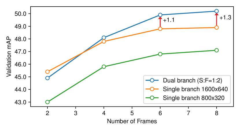
In Tab. 7, we provide detailed quanlitative results. Under the setting of 8 frames ( 4 seconds), our dual branch design with only two high resolution (HR) frames surpasses the baseline with eight HR frames. By increasing the number of HR frames to 4, we further improve the performance by 0.8 mAP and 0.5 NDS. Moreover, increasing the resolution of the LR frames does not bring any improvement, which clearly demonstrates that appearance detail and temporal motion are decoupled to different branches.
| Method | Setting | mAP | NDS |
|---|---|---|---|
| Single branch | 8f 1600 | 48.9 | 57.3 |
| Dual branch | 2f 1600 + 8f 640 | 49.4 | 57.9 |
| Dual branch | 4f 1600 + 8f 640 | 50.2 | 58.4 |
| Dual branch | 4f 1600 + 8f 800 | 50.1 | 58.0 |
Since the dual-branch design also enlarges the receptive field (smaller resolution provides larger receptive field) which may improve performance, we further analyse where the improvement comes from in Tab. 8. The first row is our baseline which takes 8 frames with a single branch of as input. We first try to increase the receptive field by adding an extra feature map (Row 2), and observe that the performance is slightly improved. This demonstrates that a larger receptive field is required for high-resolution and long-term inputs. However, the spatial appearance and temporal motion is still coupling, limiting the performance. By using dual branches of 1600 640 and 640 256 with 1:2 ratio (Row 3), we decouple spatial appearance and temporal motion, leading to better performance. Moreover, the training cost is also reduced by 1/3. This experiment demonstrates that we not only need larger receptive fields, but also decouple spatial appearance and temporal motion.
| Method | Feature Maps | Train. Cost | mAP |
|---|---|---|---|
| Single branch | 2d 17h | 48.9 | |
| Single branch | 2d 18h | 49.3 | |
| Dual branch | 1d 19h | 50.2 |
Appendix B Study on Scale-adaptive Self Attention
| Self Attention | Distance Function | NDS | mAP |
|---|---|---|---|
| SASA-beta | 55.2 | 44.8 | |
| SASA | 55.6 | 45.4 |
In this section, we’ll talk about how we came up with scale-adaptive self attention (SASA). In the main paper, the receptive field coefficient is specific to each head and adaptive to each query. In the development of SASA, there is an intermediate version (dubbed SASA-beta for convenience): the for each head is simply a learnable parameter shared by all queries.
In Fig. 9, we take a closer look at how changes with training. We surprisingly find that regardless of the initialization, each head learns a different from the others and all of them are distributed in range , enabling the network to aggregate local and multi-scale features from multiple heads.
Next, we improve SASA-beta by generating the adaptively from the query, which corresponds to the version in the main paper. Compared with SASA-beta, SASA not only has the ability of multi-scale feature aggregation, but generates adaptive receptive field for each query as well. The quanlitative comparison between SASA-beta and SASA is shown in Tab. 9.


Appendix C More Visualizations
In Fig. 10, we provide more visualizations of the sampling points from different stages. In the initial stage, the sampling points have the shape of pillars. In later stages, they are refined to cover objects with different sizes.


