Sparse Symmetric Linear Arrays with Low Redundancy and a Contiguous Sum Co-Array

Robin Rajamäki, and Visa Koivunen The authors are with the Department of Signal Processing and Acoustics, Aalto University, Espoo, Finland (e-mail: [email protected], [email protected]).This work was supported by the Academy of Finland project Massive and Sparse Antenna Array Processing for Millimeter-Wave Communications.

Abstract

Sparse arrays can resolve significantly more scatterers or sources than sensor by utilizing the co-array — a virtual array structure consisting of pairwise differences or sums of sensor positions. Although several sparse array configurations have been developed for passive sensing applications, far fewer active array designs exist. In active sensing, the sum co-array is typically more relevant than the difference co-array, especially when the scatterers are fully coherent. This paper proposes a general symmetric array configuration suitable for both active and passive sensing. We first derive necessary and sufficient conditions for the sum and difference co-array of this array to be contiguous. We then study two specific instances based on the Nested array and the Kløve-Mossige basis, respectively. In particular, we establish the relationship between the minimum-redundancy solutions of the two resulting symmetric array configurations, and the previously proposed Concatenated Nested Array (CNA) and Kløve Array (KA). Both the CNA and KA have closed-form expressions for the sensor positions, which means that they can be easily generated for any desired array size. The two array structures also achieve low redundancy, and a contiguous sum and difference co-array, which allows resolving vastly more scatterers or sources than sensors.

Index Terms:

Active sensing, sparse array configuration, symmetry, sum co-array, difference co-array, minimum redundancy.

I Introduction

Sensor arrays are a key technology in for example, radar, wireless communication, medical imaging, radio astronomy, sonar, and seismology [1]. The key advantages of arrays include spatial selectivity and the capability to mitigate interference. However, conventional uniform array configurations may become prohibitively expensive, when a high spatial resolution facilitated by a large electrical aperture, and consequently a large number of sensors is required.

Sparse arrays allow for significantly reducing the number of sensors and costly RF-IF chains, whilst resolving vastly more scatterers or signal sources than sensors. This is facilitated by a virtual array model called the co-array [2, 3], which is commonly defined in terms of the pairwise differences or sums of the physical sensor positions [3]. Uniform arrays have a co-array with redundant virtual sensors, which allows the number of physical sensors to be reduced without affecting the number of unique co-array elements. This enables sparse arrays to identify up to $\mathcal{O}(N^{2})$ signal sources using only $N$ sensors [4, 5, 6]. A contiguous co-array is often desired, since it maximizes the number of virtual sensors for a given array aperture. The properties of the resulting uniform virtual array model, such as the Vandermonde structure of the virtual steering matrix, can also be leveraged in array processing [7, 8].

Typical sparse array designs, such as the Minimum-Redundancy Array (MRA) [9, 10], seek to maximize the number of contiguous co-array elements for a given number of physical sensors $N$ . The minimum-redundancy property means that no physical array configuration can achieve a larger contiguous co-array. Although optimal, the MRA lacks a closed-form expression for its sensor positions, and quickly becomes impractical to compute, as the search space of the combinatorial optimization problem that needs to be solved grows exponentially with $N$ . Consequently, large sparse arrays have to be constructed by sub-optimal means, yielding low-redundancy, rather than provably minimum-redundancy, array configurations. For instance, smaller (but computable) MRAs can be extended to larger apertures by repeating regular substructures in the array [10], or by recursively nesting them in a fractal manner [11]. Recent research into such recursive or fractal arrays [12, 13, 14, 15] has also revived interest in symmetric array configurations. Symmetry in either the physical or co-array domain can further simplify array design [16] and calibration [17], or be leveraged in detection [18], source localization [19, 20, 21, 22], and adaptive beamforming [1, p. 721]. Parametric arrays are also of great interest, as their sensor positions can be expressed in closed form. This facilitates the simple design and optimization of the array geometry. For example, the redundancy of the array may be minimized to utilize the co-array as efficiently as possible. Notable parametric arrays include the Wichmann [23, 24, 25], Co-prime [26], Nested [7], and Super Nested Array [27, 28].

Sparse array configurations have been developed mainly for passive sensing, where the difference co-array can be exploited if the source signals are incoherent or weakly correlated. Far fewer works consider the sum co-array, which is more relevant in active sensing applications, such as radar or microwave and ultrasound imaging, where scatterers may (but need not) be fully coherent [3, 29, 30]. In particular, the design of low-redundancy sparse arrays with overlapping transmitting and receiving elements has not been extensively studied. Some of our recent works have addressed this sum co-array based array design problem by proposing symmetric extensions to existing parametric array configurations that were originally designed to only have a contiguous difference co-array [31, 32, 33]. Symmetry can thus provide a simple means of achieving a contiguous sum co-array. However, a unifying analysis and understanding of such symmetric sparse arrays is yet lacking from the literature. The current work attempts to fill this gap.

I-A Contributions and organization

This paper focuses on the design of sparse linear active arrays with a contiguous sum co-array. The main contributions of the paper are twofold. Firstly, we propose a general symmetric sparse linear array design. We establish necessary and sufficient conditions under which the sum and difference co-array of this array are contiguous. We also determine sufficient conditions that greatly simplify array design by allowing for array configurations with a contiguous difference co-array to be leveraged, thanks to the symmetry of the proposed array design. This connects our work to the abundant literature on mostly asymmetric sparse arrays with a contiguous difference co-array [25, 7, 34, 35]. Moreover, it provides a unifying framework for symmetric configurations relevant to both active and passive sensing [31, 32, 33].

The second main contribution is a detailed study of two specific instances of this symmetric array — one based on the Nested Array (NA) [7], and the other on the Kløve-Mossige basis from additive combinatorics [36]. In particular, we clarify the connection between these symmetric arrays and the recently studied Concatenated Nested Array (CNA) [37, 31] and Kløve Array (KA) [38, 33]. We also derive the minimum redundancy parameters for both the CNA and KA. Additionally, we show that the minimum-redundancy symmetric NA reduces to the CNA. Both the CNA and KA can be generated for practically any number of sensors, as their positions have closed-form expressions.

The paper is organized as follows. Section II introduces the signal model and the considered array figures of merit. Section III briefly reviews the MRA and some of its characteristics. Section IV then presents the general definition of the proposed symmetric array, and outlines both necessary and sufficient conditions for its sum co-array to be contiguous. In Section V, we study two special cases of this array, and derive their minimum-redundancy parameters. Finally, we compare the discussed array configurations numerically in Section VI, before concluding the paper and discussing future work in Section VII.

I-B Notation

We denote matrices by bold uppercase, vectors by bold lowercase, and scalars by unbolded letters. Sets are denoted by calligraphic letters. The set of integers from $a\in\mathbb{Z}$ to $c\in\mathbb{Z}$ in steps of $b\in\mathbb{N}_{+}$ is denoted $\{a:b:c\}=\{a,a+b,a+2b,\ldots,c\}$ . Shorthand $\{a:c\}$ denotes $\{a:1:c\}$ . The sum of two sets is defined as the set of pairwise sums of elements, i.e., $\mathcal{A}+\mathcal{B}\triangleq\{a+b\ |\ a\in\mathcal{A};b\in\mathcal{B}\}$ . The sum of a set and a scalar is a special case, where either summand is a set with a single element. Similar definitions hold for the difference set. The cardinality of a set $\mathcal{A}$ is denoted by $|\mathcal{A}|$ . The rounding operator $\lceil\cdot\rfloor$ quantizes the scalar real argument to the closest integer. Similarly, the ceil operator $\lceil\cdot\rceil$ yields the smallest integer larger than the argument, and the floor operator $\lfloor\cdot\rfloor$ yields the largest integer smaller than the argument.

II Preliminaries

In this section, we briefly review the active sensing and sum co-array models. We then define the considered array figure of merit, which are summarized in Table I.

II-A Signal model

Consider a linear array of $N$ transmitting and receiving sensors, whose normalized positions are given by the set of non-negative integers $\mathcal{D}\!=\!\{d_{n}\}_{n=1}^{N}\subseteq\mathbb{N}$ . The first sensor of the array is located at $d_{1}=0$ , and the last sensor at $d_{N}=L$ , where $L=\max\mathcal{D}$ is the (normalized) array aperture. This array is used to actively sense $K$ far field scatterers with reflectivities $\{\gamma_{k}\}_{k=1}^{K}\subseteq\mathbb{C}$ in azimuth directions $\{\varphi_{k}\}_{k=1}^{K}\subseteq[-\pi/2,\pi/2]$ . Each transmitter illuminates the scattering scene using narrowband radiation in a sequential or simultaneous (orthogonal MIMO) manner [29, 39]. The reflectivities are assumed fixed during the coherence time of the scene, which may consist of one or several snapshots (pulses). The received signal after a single snapshot and matched filtering is then [40]

\displaystyle\bm{x}=(\bm{A}\odot\bm{A})\bm{\gamma}+\bm{n},

(1)

where $\odot$ denotes the Khatri-Rao (columnwise Kronecker) product, $\bm{A}\!\in\!\mathbb{C}^{N\times K}$ is the array steering matrix, $\bm{\gamma}\!=\![\gamma_{1},\ldots,\gamma_{K}]^{\text{T}}\!\in\!\mathbb{C}^{K}$ is the scattering coefficient vector, and $\bm{n}\!\in\!\mathbb{C}^{N^{2}}$ is a receiver noise vector following a zero-mean white complex circularly symmetric normal distribution. A typical array processing task is to estimate parameters $\{\varphi_{k},\gamma_{k}\}_{k=1}^{K}$ , or some functions thereof, from the measurements $\bm{x}$ .

II-B Sum co-array

The effective steering matrix in (1) is given by $\bm{A}\odot\bm{A}$ . Assuming ideal omnidirectional sensors, we have

\displaystyle[\bm{A}\odot\bm{A}]_{(n-1)N+m,k}=\exp({j2\pi(d_{n}+d_{m})\delta\sin\varphi_{k}}),

where $\delta$ is the unit inter-sensor spacing in carrier wavelengths (typically $\delta=1/2$ ). Consequently, the entries of $\bm{A}\odot\bm{A}$ are supported on a virtual array, known as the sum co-array, which consists of the pairwise sums of the physical element locations.

Definition 1 (Sum co-array).

The virtual element positions of the sum co-array of physical array $\mathcal{D}$ are given by the set

\displaystyle\mathcal{D}_{\Sigma}\triangleq\mathcal{D}+\mathcal{D}=\{d_{n}+d_{m}\ |\ d_{n},d_{m}\in\mathcal{D}\}.

(2)

The relevance of the sum co-array is that it may have up to $N(N+1)/2$ unique elements, which is vastly more than the number of physical sensors $N$ . This implies that $\mathcal{O}(N^{2})$ coherent scatterers can be identified from (1), provided the set of physical sensor positions $\mathcal{D}$ is judiciously designed.

The sum co-array is uniform or contiguous, if it equals a virtual Uniform linear array (ULA) of aperture $2L=2\max\mathcal{D}$ .

Definition 2 (Contiguous sum co-array).

The sum co-array of $\mathcal{D}$ is contiguous if $\mathcal{D}+\mathcal{D}=\{0:2\max\mathcal{D}\}$ .

A contiguous co-array is desirable for two main reasons. Firstly, it maximizes the number of unique co-array elements for a given physical aperture. Second, it facilitates the use of many array processing algorithms designed for uniform arrays. For example, co-array MUSIC [7, 8] leverages the resulting Vandermonde structure to resolve more sources than sensors unambiguously in the infinite snapshot regime.

A closely related concept to the sum co-array is that of the difference co-array [2, 3]. Defined as the set of pairwise element position differences, the difference co-array mainly emerges in passive sensing applications, where the incoherence of the source signals is leveraged. Other assumptions give rise to more exotic co-arrays models, such as the difference of the sum co-array¹¹1Up to $\mathcal{O}(N^{4})$ incoherent scatterers can be resolved by utilizing the second-order statistics of (1) and the difference of the sum co-array [40]. [41, 42], and the union of the sum and difference co-array [43, 44], which are not considered herein.

II-C Array figures of merit

TABLE I: Frequently used symbols. The set of sensor positions is denoted by

\mathcal{D}

, the array aperture by

L=\max\mathcal{D}

, and the number of sensors by

N=|\mathcal{D}|

Symbol	Explanation	Value range
$\|\mathcal{D}_{\Sigma}\|$	Number of total DoFs	$\{N:2L+1\}$
$H$	Number of contiguous DoFs	$\{1:\|\mathcal{D}_{\Sigma}\|\}$
$R$	Redundancy	$[1,\infty)$
$S(d)$	$d$ -spacing multiplicity	$\{0:\min(N-1,L-d+1)\}$
$R_{\infty}$	Asymptotic redundancy	$[1,\infty)$
$F_{\infty}$	Asymptotic co-array filling ratio	$[0,1]$

II-C1 Degrees of freedom (DoF).

The number of unique elements in the sum co-array $|\mathcal{D}_{\Sigma}|$ is often referred to as the total number of DoFs. Similarly, the number of virtual elements in the largest contiguous subarray contained in the sum co-array is called the number of contiguous DoFs.

Definition 3 (Number of contiguous DoFs).

The number of contiguous DoFs in the sum co-array of $\mathcal{D}$ is

\displaystyle H\triangleq\operatorname*{arg\,max}_{h,s\in\mathbb{N}}\big{\{}h\ |\ s+\{0:h-1\}\subseteq\mathcal{D}+\mathcal{D}\big{\}}.

(3)

If the offset $s$ is zero, then $H$ equals the position of the first hole in the sum co-array. Moreover, if the sum co-array is contiguous, then $H=2L+1$ , where $L$ is the array aperture.

II-C2 Redundancy,

$R$ , quantifies the multiplicity of the co-array elements. A non-redundant array achieves $R\!=\!1$ , whereas $R\!>\!1$ holds for a redundant array.

Definition 4 (Redundancy).

The redundancy of an $N$ sensor array with $H$ contiguous sum co-array elements is

\displaystyle R\triangleq\frac{N(N+1)/2}{H}.

(4)

The numerator of $R$ is the maximum number of unique pairwise sums generated by $N$ numbers. The denominator is given by (3). Definition 4 is essentially Moffet’s definition of (difference co-array) redundancy [9] adapted to the sum co-array. It also coincides with Hoctor and Kassam’s definition [10], when the sum co-array is contiguous, i.e., $H\!=\!2L\!+\!1$ , where $2L+1$ is the aperture of the sum co-array.

II-C3 The $d$ -spacing multiplicity,

$S(d)$ , enumerates the number of inter-element spacings of a displacement $d$ in the array [45]. For linear arrays, $S(d)$ simplifies to the weight or multiplicity function [7, 46] of the difference co-array (when $d\geq 1$ ).

Definition 5 ( $d$ -spacing multiplicity [45]).

The multiplicity of inter-sensor displacement $d\geq 1$ in a linear array $\mathcal{D}$ is

\displaystyle S(d)\triangleq\frac{1}{2}\sum_{d_{n}\in\mathcal{D}}\sum_{d_{m}\in\mathcal{D}}\mathbbm{1}(|d_{n}-d_{m}|=d).

(5)

It is easy to verify that $0\leq S(d)\leq\min(N-1,L-d+1)$ , where $d\in\mathbb{N}_{+}$ . If the difference co-array is contiguous, then $S(d)\geq 1$ for $1\leq d\leq L$ .

Typically, a low value for $S(d)$ is desired for small $d$ , as sensors that are closer to each other tend to interact more strongly and exhibit coupling [17]. Consequently, the severity of mutual coupling effects deteriorating the array performance may be reduced by decreasing $S(d)$ [47, 27, 48, 35]. This simplifies array design, but has its limitations. Specifically $S(d)$ does not take into account important factors, such as the individual element gain patterns and the mounting platform, as well as the scan angle and the uniformity of the array [49, Ch. 8]. Since treating such effects in a mathematically tractable way is challenging, proxies like the number of unit spacings $S(1)$ are sometimes considered instead for simplicity.

II-C4 Asymptotic and relative quantities.

The discussed figures of merit are generally functions of $N$ , $H$ , or $L$ , i.e., they depend on the size of the array. A convenient quantity that holds in the limit of large arrays is the asymptotic redundancy

\displaystyle R_{\infty}\triangleq\lim_{N\to\infty}R=\lim_{N\to\infty}\frac{N^{2}}{2H}.

(6)

Another one is the asymptotic sum co-array filling ratio

\displaystyle F_{\infty}\triangleq\lim_{N\to\infty}\frac{H}{2L+1},

(7)

which satisfies $0\!\leq\!F_{\infty}\!\leq\!1$ , as $H\!\leq\!|\mathcal{D}_{\Sigma}|\!\leq\!2L+1$ . If the sum co-array is contiguous, then $F_{\infty}\!=\!1$ . Note that the limits in (6) and (7) may equivalently be taken with respect to $L$ or $H$ .

In many cases, we wish to evaluate the relative performance of a given array with respect to a reference array configuration of choice – henceforth denoted by superscript “ref”. Of particular interest are the three ratios

\displaystyle\frac{H}{H^{\text{ref}}},\ \frac{N}{N^{\text{ref}}}\ \text{and}\ \frac{L}{L^{\text{ref}}},

or their asymptotic values, when either $H,N$ or $L$ is equal for both arrays and approaches infinity. Table II shows that these asymptotic ratios can be expressed using (6) and (7), provided the respective limits exist. For example, the second row of the first column in Table II is interpreted as

\displaystyle\lim_{N\to\infty}\frac{H(N)}{H^{\text{ref}}(N)}=\frac{R_{\infty}^{\text{ref}}}{R_{\infty}},

where the right-hand-side follows by simple manipulations from (4). The expressions in Table II simplify greatly if both arrays have a contiguous sum co-array, since $F_{\infty}=F_{\infty}^{\text{ref}}=1$ .

TABLE II: Asymptotic ratios of the number of contiguous DoFs

H

, sensors

N

, and array aperture

L

. The variable approaching infinity is assumed equal for both arrays.

	$H/H^{\text{ref}}$	$N/N^{\text{ref}}$	$L/L^{\text{ref}}$
$H\to\infty$	$1$	$\sqrt{R_{\infty}/R_{\infty}^{\text{ref}}}$	$F_{\infty}^{\text{ref}}/F_{\infty}$
$N\to\infty$	$R_{\infty}^{\text{ref}}/R_{\infty}$	$1$	$(R_{\infty}^{\text{ref}}/R_{\infty})(F_{\infty}^{\text{ref}}/F_{\infty})$
$L\to\infty$	$F_{\infty}/F_{\infty}^{\text{ref}}$	$\sqrt{R_{\infty}/R_{\infty}^{\text{ref}}}\sqrt{F_{\infty}/F_{\infty}^{\text{ref}}}$	$1$

III Minimum-Redundancy Array

In this section, we present the sparse array design problem solved by the Minimum-redundancy array (MRA). We then review some properties of the MRA, and briefly discuss an extension that is computationally easier to find.

The MRA is defined as the solution to either of two slightly different optimization problems, depending on if the sum co-array is constrained to be contiguous or not [9].

Definition 6 (Minimum-redundancy array (MRA)).

The general Minimum-redundancy array (MRA) solves

	$\displaystyle\underset{\mathcal{D}\subseteq\mathbb{N};h\in\mathbb{N}}{\text{maximize}}$	$\displaystyle\ h$
	subject to	$\displaystyle\ \|\mathcal{D}\|=N\ \text{and}\ \mathcal{D}+\mathcal{D}\supseteq\{0:h-1\}.$		(P1)

The restricted MRA (R-MRA) is given by the solution to (P1) with the extra constraint $h=2\max\mathcal{D}+1$ .

The general MRA minimizes the redundancy $R$ , subject to a given number of sensors $N$ and offset $s=0$ in (3). By Definition 4, this is equivalent to maximizing $H$ , which by Definition 3 reduces to (P1). In contrast, the R-MRA constrains the sum co-array to be contiguous, and therefore maximizes the array aperture. A more generic definition of the general MRA is possible by including offset $s\in\mathbb{N}$ as an optimization variable in (P1). Note that the R-MRA implies that $s=0$ , regardless of the definition of the MRA. Finding general MRAs with $s\neq 0$ is an open problem that is left for future work.

MRAs can, but need not, be restricted [50, 51]. For example, two of the three MRAs with $N=8$ sensors in Table III are restricted. On the other hand, none of the general MRAs with $N=11$ sensors are restricted ( $H=47$ in the general case, respectively, $H=45$ in the restricted case) [50, 51]. The “sum MRAs” in Definition 6 are equivalent to extremal additive 2-bases, which have been extensively studied in number theory [37, 52, 36, 38, 51], similarly to difference bases [53, 23] corresponding “difference MRAs” [9]. Solving (P1) is nevertheless challenging, since the size of the search space grows exponentially with the number of elements $N$ . Consequently, MRAs are currently only known for $N\leq 25$ [50] and R-MRAs for $N\leq 48$ [54].

The MRA can also be defined for a fixed aperture. E.g., the restricted MRA would minimize $N$ subject to a contiguous co-array of length $2L+1$ . The difference MRA following this definition is referred to as the sparse ruler [55]. For a given $N$ , several such rulers of different length may exist. However, we exclusively consider the MRA of Definition 6 henceforth.

III-A Key properties

The lack of a closed-form expression for the sensor positions of the MRA make its properties difficult to analyze precisely. Nevertheless, it is straightforward to see that a linear array with a contiguous sum co-array necessarily contains two sensors in each end of the array, as shown by the following lemma.

Lemma 1 (Necessary sensors).

Let $N\geq 2$ . If $\mathcal{D}$ has a contiguous sum co-array, then $\mathcal{D}\supseteq\{0,1,L-1,L\}$ . If $\mathcal{D}$ has a contiguous difference co-array, then $\mathcal{D}\supseteq\{0,1,L\}$ .

Proof.

Clearly, $\mathcal{D}+\mathcal{D}\supseteq\{0,1,2L-1,2L\}$ if and only if $\mathcal{D}\supseteq\{0,1,L-1,L\}$ . Similarly, $\mathcal{D}-\mathcal{D}\supseteq\{0,1,L-1,L\}$ if and only if $\mathcal{D}\supseteq\{0,1,L\}$ or $\mathcal{D}\supseteq\{0,L-1,L\}$ . We may write $\mathcal{D}\supseteq\{0,1,L\}$ without loss of generality, since any $\mathcal{D}\supseteq\{0,L-1,L\}$ can be mirrored to satisfy $L-\mathcal{D}\supseteq\{0,1,L\}$ . ∎

Lemma 1 implies that any array with a contiguous sum co-array and $N\geq 4$ sensors has at least two sensor pairs separated by a unit inter-element spacing, i.e., $S(1)\geq 2$ . Lemma 1 also suggests that the R-MRA achieves redundancy $R=1$ in only two cases. These arrays are called perfect arrays.

Corollary 1 (Perfect arrays).

The only two unit redundancy R-MRAs are $\{0\}$ and $\{0,1\}$ . All other R-MRAs are redundant.

Proof.

By Lemma 1, the element at position $L$ of the sum co-array can be represented in at least two ways, namely $L=L+0=(L-1)+1$ . Consequently, if $N\geq 4$ , then $R>1$ must hold. The R-MRAs for $N\leq 3$ are $\{0\},\{0,1\}$ , and $\{0,1,2\}$ . Only the first two of these satisfy $R=1$ . ∎

Generally, the redundancy of the MRA is unknown. However, the asymptotic redundancy can be bounded as follows.

Theorem 1 (Asymptotic redundancy of MRA [56, 57, 38, 58]).

The asymptotic redundancy of the MRA satisfies

	General MRA:	$\displaystyle 1.090<R_{\infty}<1.730$
	Restricted MRA:	$\displaystyle 1.190<R_{\infty}<1.917.$

Proof.

In the general case, the lower bound $R_{\infty}\geq\frac{1}{0.917}>1.090$ follows directly from [56, Theorem 1.1], and the upper bound $R_{\infty}\leq\frac{147}{85}<1.730$ from [57, Eq. (1)]. Similarly, in the restricted case $R_{\infty}\geq\frac{11}{7+\sqrt{5}}>1.190$ [58, Theorem 1.2], and $R_{\infty}\leq\frac{23}{12}<1.917$ [38, Theorem, p. 177]. ∎

Theorem 1 suggests that the R-MRA may be more redundant than the general MRA that does not constrain the sum co-array to be contiguous. The restricted definition of the MRA is nevertheless more widely adopted than the general one for the reasons listed in Section II-B. We note that difference bases or MRAs can also be of the general or restricted type [53, 9]. Difference MRAs are typically less redundant than sum MRAs due to the commutativity of the sum, i.e., $a+b=b+a$ , but $a-b\neq b-a$ .

III-B Unique solution with fewest closely spaced sensors

Problem (P1) may have several solutions for a given $N$ , which means that the MRA is not necessarily unique [50, 51]. In order to guarantee uniqueness, we introduce a secondary optimization criterion. In particular, we consider the MRA with the fewest closely spaced sensors. This MRA is found by minimizing a weighted sum of $d$ -spacing multiplicities (see Definition 5) among the solutions to (P1), which is equivalent to subtracting a regularizing term from the objective function. This regularizer $\varsigma\geq 0$ can be defined as, for example,

\displaystyle\varsigma\triangleq\sum_{d=1}^{L}S(d)10^{-d(\lfloor\log L\rfloor+1)},

(8)

where $L\in\mathbb{N}_{+}$ is the largest aperture of the considered solutions. Consequently, any two solutions to the unregularized problem, say $\mathcal{D}_{a}$ and $\mathcal{D}_{b}$ , satisfy $\varsigma_{a}>\varsigma_{b}$ , if and only if $S_{a}(n)>S_{b}(n)$ and $S_{a}(d)=S_{b}(d)$ for all $1\leq d<n$ . In words: (8) promotes large sensor displacements by prioritizing the value of $S(1)$ , then $S(2)$ , then $S(3)$ , etc. For example, Table III shows two R-MRAs with equal $S(1)$ and $S(2)$ , but different $S(3)$ . The R-MRA with the smaller $S(3)$ , and therefore lower value of $\varsigma$ , is preferred.

TABLE III: MRAs with

N=8

sensors [50]. The bottom MRA has the fewest unit spacings. Of the two restricted MRAs, the first has fewer closely spaced sensors and hence a lower

\varsigma

Configuration	Restricted	$S(1)$	$S(2)$	$S(3)$	$\varsigma$
$\{0,1,2,5,8,11,12,13\}$	✓	$4$	$2$	$3$	$0.040203\ldots$
$\{0,1,3,4,9,10,12,13\}$	✓	$4$	$2$	$4$	$0.040204\ldots$
$\{0,1,3,5,7,8,17,18\}$	✗	$3$	$3$	$2$	$0.030302\ldots$

III-C Symmetry and the Reduced Redundancy Array

Many of the currently known sum MRAs are actually symmetric [50, 51]. In fact, there exist at least one symmetric R-MRA for each $N\leq 48$ . Moreover, the R-MRA with the fewest closely spaced sensors (lowest $\varsigma$ ) turns out to be symmetric for $N\leq 48$ . Indeed, symmetry seems to arise naturally from the additive problem structure (cf. [59, Section 4.5.3]). Note that difference MRAs are generally asymmetric [9, 11].

Imposing symmetry on the array design problem has the main advantage of reducing the size of the search space [36, 16]. In case of the MRA, this can be achieved by adding constraint $\mathcal{D}=\max\mathcal{D}-\mathcal{D}$ to (P1). Unfortunately, the search space of this symmetric MRA still scales exponentially with $N$ . Fortunately, another characteristic of the MRA may readily be exploited. Namely, MRAs tend to have a sparse mid section consisting of uniformly spaced elements [51]. The reduced redundancy array (RRA) extends the aperture of the MRA by adding extra elements to this uniform mid section [11, 10].

Definition 7 (Reduced redundancy array (RRA) [10]).

The sensor positions of the RRA for a given MRA are given by

\displaystyle\mathcal{D}_{\text{RRA}}\triangleq\mathcal{P}\cup(\mathcal{M}+\max\mathcal{P})\cup(\mathcal{S}+\max\mathcal{P}+\max\mathcal{M}),

where $\mathcal{P}$ is the prefix and $\mathcal{S}$ the suffix of the MRA, and

\displaystyle\mathcal{M}=\{0:M:(N-|\mathcal{P}|-|\mathcal{S}|+1)M\}

is the mid subarray, with inter-element spacing $M\in\mathbb{N}_{+}$ .

The prefix $\mathcal{P}$ , suffix $\mathcal{S}$ , and the inter-element spacing $M$ of $\mathcal{M}$ are determined by the generator MRA, i.e., the MRA that is extended. For example, an MRA with $N=7$ sensors is

\displaystyle\underbrace{\{0,1,2,5,8,9,10\}}_{\mathcal{D}_{\text{MRA}}}=\underbrace{\{0,1,2\}}_{\mathcal{P}}\cup\underbrace{\{2:3:8\}}_{\mathcal{M}+2}\cup\underbrace{\{8,9,10\}}_{\mathcal{S}+8}.

Note that $\mathcal{S}=\max\mathcal{P}-\mathcal{P}$ holds, if the MRAs is symmetric as above. The RRA also has a contiguous sum co-array, if the MRA is restricted.

The RRA has a low redundancy when $|\mathcal{D}_{\text{RRA}}|\approx|\mathcal{D}_{\text{MRA}}|$ . However, the redundancy of the RRA approaches infinity as $|\mathcal{D}_{\text{RRA}}|$ grows, since the aperture of the RRA only increases linearly with the number of sensors. Consequently, we will next consider a general class of symmetric arrays which scale better and admit a solution in polynomial time, provided the design space is constrained judiciously. In particular, we will show that this class of symmetric arrays naturally extends many of the established array configurations – designed for passive sensing – to the active sensing setting.

IV Symmetric array — general design and conditions for contiguous co-array

In this section, we establish a general framework for symmetric arrays with a contiguous sum (and difference) co-array. The proposed symmetric array with generator $\mathcal{G}$ (S- $\mathcal{G}$ ) is constructed by taking the union of a generator array²²2This terminology is adopted from the literature on fractal arrays [60, 14]. $\mathcal{G}$ and its mirror image shifted by a non-negative integer $\lambda$ . The generator, which is the basic construction block of the symmetric array, can be any array configuration of choice.

Definition 8 (Symmetric array with generator $\mathcal{G}$ (S- $\mathcal{G}$ )).

The sensor positions of the S- $\mathcal{G}$ are given by

\displaystyle\mathcal{D}_{\text{S-}\mathcal{G}}\triangleq\mathcal{G}\cup(\max\mathcal{G}-\mathcal{G}+\lambda),

(9)

where $\mathcal{G}$ is a generator array and $\lambda\in\mathbb{N}$ is a shift parameter³³3Note that $\lambda\leq 0$ is equivalent to considering the mirrored generator $\max{\mathcal{G}}-{\mathcal{G}}$ for $\lambda\geq 0$ . Therefore, we may set $\lambda\geq 0$ without loss of generality..

Fig. 1(a) shows a schematic of the S- $\mathcal{G}$ . Note that the number of sensors satisfies $|\mathcal{G}|\leq N\leq 2|\mathcal{G}|$ , depending on the overlap between $\mathcal{G}$ and $L-\mathcal{G}$ . The aperture $L$ of the S- $\mathcal{G}$ is

\displaystyle L=\max\mathcal{G}+\lambda.

(10)

The exact properties of the S- $\mathcal{G}$ are determined by the particular choice of $\mathcal{G}$ and $\lambda$ . Specifically, the generator array $\mathcal{G}$ influences how easily the symmetrized array S- $\mathcal{G}$ can be optimized to yield a large contiguous sum co-array. For example, a generator with a simple nested structure makes a convenient choice in this regard, as we will demonstrate in Section V. Next, however, we establish necessary and sufficient conditions that any $\mathcal{G}$ and $\lambda$ must fulfill for S- $\mathcal{G}$ to have a contiguous sum co-array. These general conditions are later utilized when considering specific choices for $\mathcal{G}$ in Section V.

IV-A Necessary and sufficient conditions for contiguous co-array

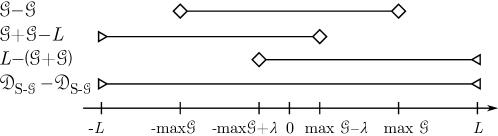
Fig. 1(b) illustrates the difference co-array of the S- $\mathcal{G}$ , which is composed of the difference co-array and shifted sum co-arrays of the generator $\mathcal{G}$ . By symmetry, the sum and difference co-array of the S- $\mathcal{G}$ are equivalent up to a shift. This fact, along with (9), allows us to express the necessary and sufficient condition for the contiguity of both co-arrays in terms of the generator $\mathcal{G}$ and shift parameter $\lambda$ . Moreover, we may conveniently decompose the condition into two simpler subconditions, as shown by the following theorem.

Theorem 2 (Conditions for contiguous co-array).

The sum (and difference) co-array of the S- $\mathcal{G}$ is contiguous if and only if

(C1)

$(\mathcal{G}-\mathcal{G})\cup(\mathcal{G}+\mathcal{G}-L)\cup(L-(\mathcal{G}+\mathcal{G}))\supseteq\{0:\max\mathcal{G}\}$
(C2)

$\mathcal{G}+\mathcal{G}\supseteq\{0:\lambda-1\},$

where $L$ is the array aperture given by (10).

Proof.

By symmetry of the physical array, the sum co-array is contiguous if and only if the difference co-array is contiguous (e.g., see [45, Lemma 1]), that is,

\displaystyle\mathcal{D}_{\text{S-}\mathcal{G}}+\mathcal{D}_{\text{S-}\mathcal{G}}=\{0:2L\}\iff\mathcal{D}_{\text{S-}\mathcal{G}}-\mathcal{D}_{\text{S-}\mathcal{G}}=\{-L:L\}.

By symmetry of the difference co-array, this is equivalent to requiring that $\mathcal{D}_{\text{S-}\mathcal{G}}\!-\!\mathcal{D}_{\text{S-}\mathcal{G}}\!\supseteq\!\{0:L\}$ , or using (9) that

	$\displaystyle\mathcal{D}_{\text{S-}\mathcal{G}}-\mathcal{D}_{\text{S-}\mathcal{G}}$	$\displaystyle=\mathcal{G}\cup(L-\mathcal{G})-\mathcal{G}\cup(L-\mathcal{G})$
		$\displaystyle=(\mathcal{G}-\mathcal{G})\cup(\mathcal{G}+\mathcal{G}-L)\cup(L-(\mathcal{G}+\mathcal{G}))$
		$\displaystyle\supseteq\{0:L\}.$

Conditions (C2) and (C1) then directly follow from (10). ∎

Note that (C2) may also be reformulated as $\lambda\leq H$ , where $H$ denotes the position of the first hole in the sum co-array of $\mathcal{G}$ , per (3). Since $H\leq 2\max\mathcal{G}+1$ , the sum co-array of $\mathcal{D}_{\text{S-}\mathcal{G}}$ is contiguous only if $\lambda$ satisfies

\displaystyle\lambda\leq 2\max\mathcal{G}+1.

IV-B Sufficient conditions for contiguous co-array

It is also instructive to consider some simple sufficient conditions for satisfying (C1) and (C2), as outlined in the following two corollaries to Theorem 2.

Corollary 2 (Sufficient conditions for (C1)).

Condition (C1) is satisfied if either of the following holds:

(i)

$\mathcal{G}$ has a contiguous difference co-array.
(ii)

$\mathcal{G}$ has a contiguous sum co-array and $\lambda\leq\max\mathcal{G}+1$ .

Proof.

Firstly, if the difference co-array of $\mathcal{G}$ is contiguous, then $\mathcal{G}-\mathcal{G}\supseteq\{0:\max\mathcal{G}\}$ holds by definition, implying (C1). Secondly, if the sum co-array is contiguous, then $\mathcal{G}+\mathcal{G}\supseteq\{0:2\max\mathcal{G}\}$ holds, which implies that

	$\displaystyle\mathcal{G}+\mathcal{G}-L$	$\displaystyle=\{-L:\max\mathcal{G}-\lambda\}$
	$\displaystyle L-(\mathcal{G}+\mathcal{G})$	$\displaystyle=\{-\max\mathcal{G}+\lambda:L\}.$

If $\lambda\leq\max\mathcal{G}+1$ , then the union of these two sets and $\mathcal{G}-\mathcal{G}$ covers $\{-L:L\}\supseteq\{0:\max\mathcal{G}\}$ , implying (C1). ∎

Corollary 3 (Sufficient conditions for (C2)).

Condition (C2) is satisfied if any of the following hold:

(i)

$\lambda\leq 1$
(ii)

$\lambda\leq 3$ and $|\mathcal{G}|\geq 2$
(iii)

$\lambda\leq 2\max\mathcal{G}+1$ and $\mathcal{G}$ has a contiguous sum co-array.

Proof.

Firstly, $\lambda\leq 1$ implies (C2), since $\mathcal{G}\supseteq\{0\}$ . Secondly, if $|\mathcal{G}|\geq 2$ , then $\mathcal{G}\supseteq\{0,1\}$ holds by Lemma 1. Consequently, $|\mathcal{G}|\geq 2$ and $\lambda\leq 3\implies$ (C2). Thirdly, if $\mathcal{G}$ has a contiguous sum co-array and $\lambda\leq 2\max\mathcal{G}+1$ , then $\mathcal{G}\!+\!\mathcal{G}\!=\!\{0:2\max\mathcal{G}\}\supseteq\{0:\lambda\!-\!1\}$ holds by definition. ∎

We note that if $|\mathcal{G}|\geq 2$ , then $\lambda\leq\max\mathcal{G}+2$ is actually sufficient in Item (ii) of Corollary 2 (cf. Lemma 1). This is also sufficient for satisfying (C2) by Item (iii) of Corollary 3. Item (i) of Corollary 2 is of special interest, since it states that any $\mathcal{G}$ with a contiguous difference co-array satisfies (C1). This greatly simplifies array design, as shown in the next section, where we develop two arrays leveraging this property.

Refer to caption — (a) Physical array and constituent sub-arrays

V Low-redundancy symmetric array designs using parametric generators

Similarly to the R-MRA in (P1), we wish to find the S- $\mathcal{G}$ with maximal aperture satisfying the conditions in Theorem 2. Given a number of elements $N$ , and a class of generator arrays $\mathscr{G}$ , such that $\mathcal{G}\in\mathscr{G}$ , this minimum-redundancy S- $\mathcal{G}$ design is found by solving the following optimization problem:

$\displaystyle\underset{\mathcal{G}\in\mathscr{G},\lambda\in\mathbb{N}}{\text{maximize}}$	$\displaystyle\ \max\mathcal{G}+\lambda$
subject to	$\displaystyle\ \|\mathcal{G}\cup(\max\mathcal{G}-\mathcal{G}+\lambda)\|=N$
	$\displaystyle\ \text{\ref{c:gmg} and \ref{c:gpg}}.$	(P2)

In general, (P2) is a non-convex problem, whose difficulty depends on the choice of $\mathscr{G}$ . Solving (P2) may therefore require a grid search over $\lambda$ and the elements of $\mathscr{G}$ , which can have exponential complexity at worst. At best, however, a solution can be found in polynomial time, or even in closed form.

We will now focus on a family of choices for $\mathscr{G}$ , such that each $\mathcal{G}\in\mathscr{G}$ has the following two convenient properties:

(a)

$\mathcal{G}$ has a contiguous difference co-array
(b)

$\mathcal{G}$ has a closed-form expression for its aperture.

Item (a) greatly simplifies (P2) by directly satisfying condition (C1), whereas Item (b) enables the straightforward optimization of the array parameters. Condition (C2) is typically easy to satisfy for an array with these two properties. This is the case with many sparse array configurations in the literature, such as the Nested [7] and Wichmann Array [23, 24, 25]. Constructing a symmetric array using a generator with a contiguous difference co-array is thus a practical way to synthesize a contiguous sum co-array.

V-A Symmetric Nested Array (S-NA)

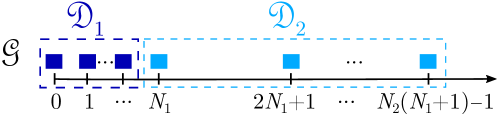
The Nested Array (NA) [7] is a natural choice for a generator satisfying the previously outlined properties (a) and (b). The NA has a simple structure consisting of the union of a dense ULA, $\mathcal{D}_{1}$ , and sparse ULA sub-array, $\mathcal{D}_{2}$ , as shown in Fig. 2(a). When used as the generator $\mathcal{G}$ in (9), the NA yields the Symmetric Nested Array (S-NA), defined as follows:

Definition 9 (Symmetric Nested Array (S-NA)).

The sensor positions of the S-NA are given by (9), where

\displaystyle\mathcal{G}=\mathcal{D}_{1}\cup(\mathcal{D}_{2}+N_{1}),

with $\mathcal{D}_{1}=\{0:N_{1}-1\};$ $\mathcal{D}_{2}=\{0:N_{1}+1:(N_{2}-1)(N_{1}+1)\}$ ; and array parameters $N_{1},N_{2}\in\mathbb{N}$ .

Special cases of the S-NA have also been previously proposed. For example, [61, Definition 2] considered the case $\lambda=0$ for improving the robustness of the NA to sensor failures. Next we briefly discuss a special case that is more relevant from the minimum-redundancy point of view.

V-A1 Concatenated Nested Array (CNA)

The S-NA coincides with a restricted additive 2-basis studied by Rohrbach in the 1930’s [37, Satz 2], when the shift parameter $\lambda$ satisfies

\displaystyle\lambda=(N_{1}+1)k+N_{1},

(11)

where $k\in\{0:N_{2}\}$ . Unaware of Rohrbach’s early result, we later derived the same configuration based on the NA and called it the Concatenated Nested Array (CNA) [31].

Definition 10 (Concatenated Nested Array (CNA) [31]).

The sensor positions of the CNA are given by

\displaystyle\mathcal{D}_{\text{CNA}}\triangleq\mathcal{D}_{1}\cup(\mathcal{D}_{2}+N_{1})\cup(\mathcal{D}_{1}+N_{2}(N_{1}+1)),

where $N_{1},N_{2}\in\mathbb{N}$ , and $\mathcal{D}_{1},\mathcal{D}_{2}$ follow Definition 9.

The CNA is illustrated in Fig. 2(c). When $N_{1}=0$ or $N_{2}\in\{0,1\}$ , the array degenerates to the ULA. In the interesting case when $N_{1}+N_{2}\geq 1$ , the aperture of the CNA is[31]

\displaystyle L

\displaystyle=(N_{1}+1)(N_{2}+1)-2.

(12)

Furthermore, the number of sensors is [31]

\displaystyle N=\begin{cases}N_{1},&\text{if }N_{2}=0\\ 2N_{1}+N_{2},&\text{otherwise,}\end{cases}

(13)

and the number of unit spacings evaluates to

\displaystyle S(1)

\displaystyle=\begin{cases}N_{1}-1,&\text{if }N_{2}=0\\ N_{2}-1,&\text{if }N_{1}=0\\ 2N_{1},&\text{otherwise}.\end{cases}

(14)

V-A2 Minimum-redundancy solution

The S-NA solving (P2) is actually a CNA. This follows from the fact that any S-NA that has a contiguous sum co-array, but is not a CNA, has redundant sensors, due to the reduced number of overlapping sensors between $\mathcal{G}$ and its shifted mirror image.

Proposition 1.

The S-NA solving (P2) is a CNA.

Proof.

We write (C1) and (C2) as a constraint on $\lambda$ , which we then show implies the proposition under reparametrization.

Firstly, (C1) holds by Item (i) of Corollary 2, since the NA has a contiguous difference co-array [7]. Secondly, the location of the first hole in the sum co-array of the NA yields that (C2) is satisfied if and only if

\displaystyle\lambda\leq\begin{cases}2(N_{1}+N_{2})-1,&\text{ if }N_{1}=0\text{ or }N_{2}=0\\ N_{2}(N_{1}+1)+N_{1},&\text{ otherwise}.\end{cases}

(15)

If $0\leq\lambda\leq N_{1}-1$ , then a CNA with the same number of sensors ( $N=2|\mathcal{G}|-2$ ), but a larger aperture ( $L=\max\mathcal{G}+\lambda$ ) is achieved by instead setting $\lambda=\max\mathcal{G}-N_{1}$ . Otherwise, it is straightforward to verify that the S-NA either reduces to the CNA, or a CNA can be constructed with the same $N$ but a larger $L$ , by satisfying (15) with equality. ∎

By Proposition 1, problem (P2) simplifies to maximizing the aperture of the CNA for a given number of sensors:

\displaystyle\underset{N_{1}\in\mathbb{N},N_{2}\in\mathbb{N}_{+}}{\text{maximize}}

\displaystyle\ N_{1}N_{2}+N_{1}+N_{2}\ \ \text{s.t.}\ \ 2N_{1}+N_{2}=N.

(P3)

Problem (P3) actually admits a closed-form solution [31]. In fact, we may state the following more general result for any two-variable integer program similar to (P3).

Lemma 2.

Let $f$ be a concave function. The solution to

\displaystyle\underset{x,y\in\mathbb{N}}{\text{maximize}}\ f(x,y)\ \text{subject to}\ g(x)=y

(P4)

is given by $x=\lceil z\rfloor+k$ and $y=g(x)$ , where $z$ solves

\displaystyle\underset{z\in\mathbb{R}_{+}}{\text{maximize}}

\displaystyle\ f(z,g(z)),

and $|k|$ is the smallest non-negative integer satisfying $g(\lceil z\rfloor+k)\in\mathbb{N}$ , where $k\in\{-\lceil z\rfloor,-\lceil z\rfloor+1,\ldots,-1\}\cup\mathbb{N}$ .

Proof.

Since $f(z,g(z))$ is concave, $x=\lceil z\rfloor$ maximizes $f(x,g(x))$ among all $x\in\mathbb{N}$ . This is a global optimum of (P4), if $g(\lceil z\rfloor)\in\mathbb{N}$ . Generally, the optimal solution can be expressed as $x=\lceil z\rfloor+k$ , where $k\in\{-\lceil z\rfloor:-1\}\cup\mathbb{N}$ . By concavity of $f$ , the smallest $|k|$ satisfying $g(\lceil z\rfloor+k)\in\mathbb{N}$ then yields the global optimum of (P4). ∎

Lemma 2 is useful for solving two-variable integer programs similar to (P3) in closed-form. Such optimization problems often arise in, e.g., sparse array design [32, 33]. In our case, Lemma 2 allows expressing the minimum-redundancy parameters of the CNA directly in terms of $N$ as follows⁴⁴4An equivalent result is given in [37, Eq. (7) and (8)] and [31, Eq. (13)], but in a more inconvenient format due to the use of the rounding operator..

Theorem 3 (Minimum-redundancy parameters of CNA).

The parameters of the CNA solving (P3) are

	$\displaystyle N_{1}$	$\displaystyle=(N-\alpha)/4$		(16)
	$\displaystyle N_{2}$	$\displaystyle=(N+\alpha)/2,$		(17)

where $N=4m+k,m\in\mathbb{N},k\in\{0:3\}$ , and

\displaystyle\alpha=(k+1)\bmod 4-1.

(18)

Proof.

By Lemma 2, the optimal solution to (P3) is given by $N_{1}=\lceil(N-1)/4\rfloor$ and $N_{2}=N-2N_{1}$ [31]. Since any $N\in\mathbb{N}$ may be expressed as $N=4m+k$ , where $m\in\mathbb{N}$ and $k\in\{0:3\}$ , we have

\displaystyle N_{1}=\Big{\lceil}m+\frac{k-1}{4}\Big{\rfloor}=\begin{cases}m,&k\in\{0,1,2\}\\ m+1,&k=3.\end{cases}

Since $m=(N-k)/4$ , we have $N_{1}=m=(N-k)/4$ , when $k\in\{0,1,2\}$ . Similarly, when $k=3$ , we have $N_{1}=m+1=(N-k+4)/4=(N+1)/4$ , which yields (16) and (18). Substituting (16) into (13) then yields (17). ∎

By Theorem 3, the properties of the minimum-redundancy CNA can also be written compactly as follows.

Corollary 4 (Properties of minimum-redundancy CNA).

The aperture $L$ , number of sensors $N$ , and number of unit spacings $S(1)$ of the CNA solving (P3) are

	$\displaystyle L$	$\displaystyle=(N^{2}+6N-7)/8-\beta$
	$\displaystyle N$	$\displaystyle=2\sqrt{2}\sqrt{L+2+\beta}-3$
	$\displaystyle S(1)$	$\displaystyle=(N-\alpha)/2,$

where $\beta=(\alpha-1)^{2}/8$ and $\alpha$ is given by (18).

Proof.

This follows from Theorem 3, and (12)–(14). ∎

V-B Symmetric Kløve-Mossige array (S-KMA)

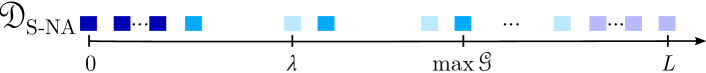
In the 1980’s, Kløve and Mossige proposed an additive 2-basis with some interesting properties [36]. In particular, the basis has a contiguous difference co-array (see Appendix A) and a low asymptotic redundancy ( $R_{\infty}\!=\!1.75$ ), despite having a non-contiguous sum co-array (see Appendix B). We call this construction the Kløve-Mossige Array (KMA). As shown in Fig. 3(a), the KMA contains a CNA, and can therefore be interpreted as another extension of the NA. However, selecting the KMA as the generator in (9) yields the novel Symmetric Kløve-Mossige Array (S-KMA), shown in Fig. 3(b).

Definition 11 (Symmetric Kløve-Mossige Array (S-KMA)).

The sensor positions of the S-KMA are given by (9), where

	$\displaystyle\mathcal{G}$	$\displaystyle=\mathcal{D}_{\text{CNA}}\cup(\mathcal{D}_{3}+2\max\mathcal{D}_{\text{CNA}}+1),$
	$\displaystyle\mathcal{D}_{3}$	$\displaystyle=\{0:N_{1}:N_{1}^{2}\}+\bigcup_{i=1}^{N_{3}}\{(i-1)(N_{1}^{2}+\max\mathcal{D}_{\text{CNA}}+1)\},$

$\mathcal{D}_{\text{CNA}}$ follows Definition 10, and parameters⁵⁵5The S-KMA is undefined for $N_{1}=N_{2}=0$ , as $\mathcal{D}_{\text{CNA}}=\emptyset$ . Consequently, we will not consider this case further. However, we note that Definition 11 is easily modified so that the S-KMA degenerates to a ULA even in this case. $N_{1},N_{2},N_{3}\!\in\!\mathbb{N}$ .

V-B1 Kløve array

The structure of the S-KMA simplifies substantially when the shift parameter $\lambda$ is of the form

\displaystyle\lambda=2\max\mathcal{D}_{\text{CNA}}+1+(\max\mathcal{D}_{\text{CNA}}+N_{1}^{2})k,

(19)

where $k\!\in\!\{0\!:\!N_{3}\}$ . In fact, this S-KMA coincides with the Kløve array (KA), which is based on a class of restricted additive 2-bases proposed by Kløve in the context of additive combinatorics [38] (see also [33]).

Definition 12 (Kløve array (KA) [38]).

The sensor positions of the KA with parameters $N_{1},N_{2},N_{3}\!\in\!\mathbb{N}$ are given by

	$\displaystyle\mathcal{D}_{\text{KA}}\triangleq$	$\displaystyle\ \mathcal{D}_{\text{CNA}}\cup(\mathcal{D}_{3}+2\max\mathcal{D}_{\text{CNA}}+1)$
		$\displaystyle\cup(\mathcal{D}_{\text{CNA}}+(N_{3}+2)\max\mathcal{D}_{\text{CNA}}+N_{3}(N_{1}^{2}+1)+1),$

where $\mathcal{D}_{\text{CNA}}$ follows Definition 10, and $\mathcal{D}_{3}$ Definition 11.

Fig. 3(c) illustrates the KA, which consists of two CNAs connected by a sparse mid-section consisting of $N_{3}$ widely separated and sub-sampled ULAs with $N_{1}+1$ elements each. The KA reduces to the CNA when $N_{1}=0$ or $N_{2}=0$ . When $N_{2}\geq 1$ , the aperture $L$ , and the number of sensors $N$ of the KA evaluate to [38, Lemma 3]:

	$\displaystyle L$	$\displaystyle=(N_{1}+1)(N_{3}(N_{1}+N_{2})+3N_{2}+3)-5$		(20)
	$\displaystyle N$	$\displaystyle=2(2N_{1}+N_{2})+N_{3}(N_{1}+1).$		(21)

Furthermore, the number of unit spacings $S(1)$ is [33]

\displaystyle S(1)

\displaystyle=\begin{cases}N_{3}+1,&\text{if }N_{1}=0\text{ and }N_{2}=1\\ 2(N_{2}-1),&\text{if }N_{1}=0\text{ and }N_{2}\geq 2\\ N_{3}+4,&\text{if }N_{1}=1\\ 4N_{1},&\text{otherwise.}\end{cases}

(22)

V-B2 Minimum-redundancy solution

The simple structure of the KMA suggests that the minimum redundancy S-KMA is also a KA. Intuitively, any S-KMA that is not a KA is unnecessarily redundant, since increasing $\lambda$ to its maximum value $H$ yields a KA (cf. Appendix B). However, proving that the S-KMA solving (P2) is a KA is not as simple as in the case of the S-NA and CNA (see Proposition 1 in Section V-A2). In particular, the S-KMA cannot easily be modified into a KA with an equal or larger aperture without affecting the number of sensors $N$ . A formal proof is therefore still an open problem.

Nevertheless, we may derive the minimum redundancy parameters of the KA. The minimum-redundancy Kløve array (KA_R) maximizes the aperture for a given $N$ , which is equivalent to solving the following optimization problem:

	$\displaystyle\underset{N_{1},N_{3}\in\mathbb{N},N_{2}\in\mathbb{N}_{+}}{\text{maximize}}$	$\displaystyle\ 3N_{1}(N_{2}+1)+3N_{2}+N_{3}(N_{1}+N_{2})(N_{1}+1)$
	subject to	$\displaystyle\ 2(2N_{1}+N_{2})+N_{3}(N_{1}+1)=N.$		(P5)

Problem (P5) is an integer program with three unknowns. This problem is challenging to solve in closed form for any $N$ , in contrast to (P3), which only has two integer unknowns (cf. Theorem 3). Nevertheless, some $N$ readily yield a closed-form solution to (P5), as shown by the following theorem.

Theorem 4 (Minimum-redundancy parameters of KA).

The parameters of the KA solving (P5) are

$\displaystyle N_{1}$	$\displaystyle=(N+3)/23$	(23)
$\displaystyle N_{2}$	$\displaystyle=5(N+3)/23$	(24)
$\displaystyle N_{3}$	$\displaystyle=(9N-42)/(N+26),$	(25)

when $N\!\in\!\{20,43,66,112,250\}$ .

Proof.

Under certain conditions, we may obtain a solution to (P5) by considering a relaxed problem. Specifically, solving (21) for $N_{3}$ , substituting the result into (20), and relaxing $N_{1},N_{2}\in\mathbb{R}$ leads to the following concave quadratic program:

\displaystyle\underset{N_{1},N_{2}\in\mathbb{R}}{\text{maximize}}

\displaystyle\ (N_{1}+N_{2})(N\!+\!3)-3N_{1}N_{2}-4N_{1}^{2}-2N_{2}^{2}.

At the critical point of the objective function we have

	$\displaystyle\partial L/\partial N_{1}$	$\displaystyle=N-8N_{1}-3N_{2}+3=0$
	$\displaystyle\partial L/\partial N_{2}$	$\displaystyle=N-3N_{1}-4N_{2}+3=0.$

Solving these equations for $N_{1}$ and $N_{2}$ yields (23) and (24), which when substituted into (21) yields (25). These are also solutions to (P5) if:

(i)

$N_{1}\in\mathbb{N}$ , which holds when $N=23k-3,k\in\mathbb{N}_{+}$ , i.e., $N=20,43,66,89,112,135,158,181,204,227,250,\ldots$
(ii)

$N_{2}\in\mathbb{N}$ , which holds when $N_{1}\in\mathbb{N}$ , as $N_{2}=5N_{1}\in\mathbb{N}$
(iii)

$N_{3}\in\mathbb{N}$ , which holds when $N=(26l+42)/(9-l)\in\mathbb{N}$ and $l\in\{0:8\}$ , i.e., $N=20,43,66,112,250$ .

The only integer-valued $N$ satisfying all three conditions are $N\!=\!20,43,66,112,250$ , as stated.

The KA in Theorem 4 also has the following properties:

Corollary 5 (Properties of minimum-redundancy KA).

The aperture $L$ , number of sensors $N$ , and number of unit spacings $S(1)$ of the KA solving (P5) are

	$\displaystyle L$	$\displaystyle=(3N^{2}+18N-19)/23$
	$\displaystyle N$	$\displaystyle=\sqrt{23/3}\sqrt{L+2}-3$
	$\displaystyle S(1)$	$\displaystyle=\begin{cases}(N+22)/6&N_{1}=1\\ 4(N+3)/23&N_{1}\geq 2,\end{cases}$

when $N\!\in\!\{20,43,66,112,250\}.$

Proof.

This follows from Theorem 4 and (20)–(22). ∎

The minimum-redundancy KA achieves the asymptotic redundancy $R_{\infty}\!=\!23/12$ , as shown in the following proposition, which is a reformulation of [38, Theorem, p. 177].

Proposition 2 (Asymptotic redundancy of KA [38]).

The asymptotic redundancy of the solution to (P5) is

\displaystyle R_{\infty}=23/12<1.9167.

Proof.

Let $N=23k+9$ , where $k\in\mathbb{N}$ . A feasible KA that is equivalent to the minimum-redundancy KA when $N\to\infty$ is then given by the choice of parameters $N_{1}=(N-9)/23$ , $N_{2}=5N_{1}$ , and $N_{3}=9$ . Substitution of these parameters into (20) yields $L=3N^{2}/23+\mathcal{O}(N)$ , i.e., $R_{\infty}=23/12$ . ∎

V-B3 Polynomial time grid search

Although solving (P5) in closed form for any $N$ is challenging, we can nevertheless obtain the solution in at most $\mathcal{O}(N\log N)$ objective function evaluations. This follows from the fact that the feasible set of (P5) only has $\mathcal{O}(N\log N)$ or fewer elements.

Proposition 3 (Cardinality of feasible set in (P5)).

The cardinality of the feasible set in (P5) is at most $\mathcal{O}(N\log N)$ .

Proof.

We may verify from (21) that $0\leq N_{1}\leq(N-2)/4$ and $0\leq N_{3}\leq(N-4N_{1})/(N_{1}+1)$ . Consequently, the number of grid points that need to be checked is

\displaystyle V=\sum_{N_{1}=0}^{\lfloor\frac{N-2}{4}\rfloor}\Bigg{\lfloor}\frac{N-4N_{1}}{N_{1}+1}\Bigg{\rfloor}+1\leq\int_{0}^{\frac{N+2}{4}}\frac{N-3x+5/2}{x+1/2}dx.

The upper bound follows from ignoring the floor operations, and substituting $N_{1}\!=\!x\!-\!1/2$ , where $x\!\in\!\mathbb{R}$ , to account for the rectangular integration implied by the sum. Finally,

V\!\leq\!(N\!+\!4)\log(N/2\!+\!2)\!-\!3(N\!+\!2)/4\!=\!\mathcal{O}(N\log N)

follows from integration by parts.

Algorithm 1 summarizes a simple grid search that finds the solution to (P5) for any $N$ in $\mathcal{O}(N\log N)$ steps, as implied by Proposition 3. We iterate over $N_{1}$ and $N_{3}$ , because this choice yields the least upper bound on the number of grid points that need to be checked⁶⁶6Selecting $N_{1}$ and $N_{2}$ , or $N_{2}$ and $N_{3}$ , yields $\mathcal{O}(N^{2})$ points.. Since the solution to (P5) is not necessarily unique, we select the KA_R with the fewest closely spaced sensors, similarly to the MRA in Section III-B. Note that computing the regularizer $\varsigma$ requires $\mathcal{O}(N^{2})$ floating point operations (flops), whereas evaluating the aperture $L$ only requires $\mathcal{O}(1)$ flops. Consequently, the time complexity of finding the KA_R with the fewest closely spaced sensors is⁷⁷7Actually, $\varsigma$ only needs to be computed when $L\!=\!L^{\star}$ in Algorithm 1. $\mathcal{O}(N^{2})$ , whereas finding any KA_R, that is, solving (P5) in general, has a worst case complexity of $\mathcal{O}(N\log N)$ .

Algorithm 1 Minimum-redundancy parameters of Kløve Array

1:procedure KA_R(

N

)

f\leftarrow-\infty

\triangleright

initialize objective function value

3: for

N_{1}\in\{0:\lfloor(N-2)/4\rfloor\}

4: for

N_{3}\in\{0:\lfloor(N-4N_{1})/(N_{1}+1)\rfloor\}

N_{2}\leftarrow(N-(N_{1}+1)N_{3})/2-2N_{1}

6: if

{N_{2}\bmod 1\!=\!0}

then

\triangleright

N_{2}

valid if integer

7: Compute

L

and

\varsigma

using (20) and (8)

8: if

L-\varsigma>f

then

\triangleright

better solution found

f\leftarrow L-\varsigma

\triangleright

update objective fcn.

10: for

i\in\{1:3\}

N_{i}^{\star}\leftarrow N_{i}

11: return

N_{1}^{\star},N_{2}^{\star},N_{3}^{\star}

\triangleright

optimal array parameters

In a recent related work, we also developed a KA with a constraint on the number of unit spacings [33]. This constant unit spacing Kløve Array (KA_S) achieves $S(1)=8$ for any $N$ at the expense of a slight increase in redundancy (asymptotic redundancy $R_{\infty}=2$ ). The minimum-redundancy parameters of the KA_S are found in closed form by application of Lemma 2, similarly to the CNA (cf. [33, Theorem 1]).

V-C Other generator choices

Naturally, other choices for the generator $\mathcal{G}$ may yield alternative low-redundancy symmetric array configurations. For example, the Wichmann generator with $\lambda=0$ yields the Interleaved Wichmann Array (IWA) [32]. This array satisfies (C1) by Item (i) of Corollary 2 and (C2) by Item (i) of Corollary 3. The IWA has the same asymptotic redundancy as the CNA, but fewer unit spacings. Although finding the minimum-redundancy parameters of the more general Symmetric Wichmann Array (S-WA) in closed-form is cumbersome, numerical optimization of $\lambda$ and the other array parameters can slightly improve the non-asymptotic redundancy of the S-WA compared to the IWA. Nevertheless, neither the IWA nor S-WA are considered further in this work, since the KA achieves both lower $R$ and $S(1)$ .

Numerical experiments suggest that some prominent array configurations, such as the Super Nested Array [27] or Co-prime Array [26], are not as well suited as generators $\mathcal{G}$ from the redundancy point of view (mirroring $\mathcal{G}$ does not help either). However, several other generators, both with and without contiguous difference co-arrays, remain to be explored in future work. For example, the difference MRA [9] and minimum-hole array [62, 63] are interesting candidates.

VI Performance evaluation of array designs

In this section, we compare the sparse array configurations presented in Sections III and V in terms of the array figures of merit in Section II-C. We also demonstrate the proposed sparse array configurations’ capability of resolving more scatterers than sensors in an active sensing scenario. Further numerical results can be found in the companion paper [33].

VI-A Comparison of array figures of merit

Tables IV and V summarize the key properties and figures of merit of the discussed sparse array configurations. The parameters of each configuration is chosen such that they maximize the number of contiguous DoFs $H$ in (3). The optimal parameters of the NA and KMA are found similarly to those of the CNA and KA (cf. Theorems 3 and 4)⁸⁸8Derivations are straightforward and details are omitted for brevity.. Fig. 4 illustrates the array configurations for $N=24$ sensors. The RRA is omitted since the MRA is known in this case. Note that the sum and difference co-arrays of the symmetric arrays are contiguous and merely shifted copies of each other.

[t] Array configuration Symmetric Contiguous DoFs^a, $H$ Total DoFs, $|\mathcal{D}_{\Sigma}|$ Aperture, $L$ No. of sensors, $N$ No. of unit spacings, $S(1)$ General Minimum-Redundancy Array (MRA) no n/a n/a $\geq(H-1)/2$ and $\leq H$ n/a $\geq 1$ Nested Array (NA) [7] no $(N^{2}+2N-4)/4$ $H+N/2-1$ $(N^{2}+4N)/4$ $\sqrt{4L+5}-1$ $N/2$ Kløve-Mossige Array (KMA) [36] no $(2N^{2}+8N+1)/7$ $H+6N/7+\mathcal{O}(1)$ $(11N^{2}+16N-61)/49$ $(7\sqrt{11L+15}-8)/11$ $2(N+2)/7$ \hdashlineRestricted Minimum-Redundancy Array (R-MRA) no^b n/a $H$ $(H-1)/2$ n/a $\geq 2$ Reduced-Redundancy Array (RRA) [10] yes $30N-706$ $H$ $15N-353$ $(L+353)/15$ $10$ Concatenated Nested Array (CNA) [31] yes $(N^{2}+6N-3)/4$ $H$ $(N^{2}+6N-7)/8$ $2\sqrt{2}\sqrt{L+2}-3$ $N/2-1/2$ Constant unit spacing Kløve Array (KA_S) [33] yes $(N^{2}+10N-83)/4$ $H$ $(N^{2}+10N-87)/8$ $2\sqrt{2}\sqrt{L+14}-5$ $8$ Minimum-Redundancy Kløve Array (KA_R) yes $(6N^{2}+36N-15)/23$ $H$ $(3N^{2}+18N-19)/23$ $\sqrt{23/3}\sqrt{L+2}-3$ $4N/23+12/23$

a

The tabulated results are representative of the scaling with $N$ or $L$ for the parameters maximizing $H$ . The expressions only hold exactly for specific values of $N$ and $L$ , which may vary between configurations.
b

The R-MRA has both asymmetric and symmetric solutions. A symmetric solution exists at least for all $N\leq 48$ .

TABLE IV: Key properties of considered sparse array configurations. The arrays below the dashed line have a contiguous sum co-array. The symmetric arrays have equivalent sum and difference co-arrays.

TABLE V: Asymptotic array figures of merit. The KA_R has at most

27\%

more sensors than the R-MRA, which is less than other known arrays with closed-form sensor positions and a contiguous sum co-array.

Array	$R_{\infty}$	$F_{\infty}$	$\lim H/H^{\text{R-MRA}}$		$\lim N/N^{\text{R-MRA}}$		$\lim L/L^{\text{R-MRA}}$
Array	$R_{\infty}$	$F_{\infty}$	$N\to\infty$	$L\to\infty$	$H\to\infty$	$L\to\infty$	$H\to\infty$	$N\to\infty$
MRA	$1.09-1.73$	$0.5-1$	$1-1.76$	$0.5-1$	$0.75-1$	$0.53-1$	$1-2$	$1-3.52$
NA	$2$	$0.5$	$0.60-0.96$	$0.5$	$1.02-1.30$	$0.72-0.92$	$2$	$1.19-1.92$
KMA	$1.75$	$0.64$	$0.68-1.10$	$0.64$	$0.96-1.21$	$0.76-0.97$	$1.57$	$1.07-1.72$
\hdashlineR-MRA	$1.19-1.92$	$1$	$1$	$1$	$1$		$1$	$1$
RRA	$\infty$	$1$	$0$	$1$	$\infty$		$1$	$0$
CNA	$2$	$1$	$0.60-0.96$	$1$	$1.02-1.30$		$1$	$0.60-0.96$
KA_S	$2$	$1$	$0.60-0.96$	$1$	$1.02-1.30$		$1$	$0.60-0.96$
KA_R	$1.92$	$1$	$0.62-1$	$1$	$1-1.27$		$1$	$0.62-1$

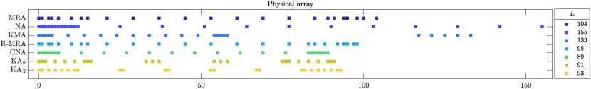
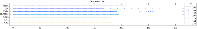
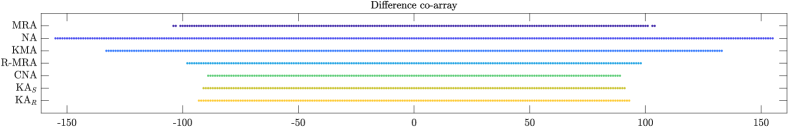
VI-A1 Non-contiguous sum co-array

We first briefly consider the configurations with a non-contiguous sum co-array before studying the arrays with a contiguous sum co-array in more detail. Note from Table IV that even when the sum co-array is non-contiguous, the number of total DoFs $|\mathcal{D}_{\Sigma}|$ is only slightly larger than the number of contiguous DoFs $H$ . Specifically, the difference between the two is proportional to the number of physical sensors $N$ , which is much smaller than $H\propto N^{2}$ , especially when $N$ or $H$ grow large. Table V shows that for the same number of contiguous DoFs $H\to\infty$ , the general MRA has at most $25\%$ fewer sensors than the R-MRA by the most conservative estimate. For a fixed aperture $L\to\infty$ , the corresponding number is at most $47\%$ , mainly due to the uncertainty related to $L$ , and thus the asymptotic co-array filling ratio $F_{\infty}$ , of the general MRA. In particular, any configuration seeking to maximize $H$ , such as the MRA, must satisfy $H\geq L$ . Moreover, $H\leq 2L+1$ holds by definition.

Among the considered configurations with closed-form sensor positions, the KMA achieves the largest number of contiguous DoFs $H$ , and therefore the lowest redundancy⁹⁹9The construction in [57] achieves an approximately $1\%$ lower $R_{\infty}$ . for a fixed number of sensors $N$ . However, its sum co-array contains holes, since $F_{\infty}=7/11<1$ . For equal aperture $L\to\infty$ , the KA_R has a $57\%$ larger $H$ than the KMA, but only $31\%$ more physical sensors $N$ . Similarly, the CNA has a two times larger $H$ than the NA and $41\%$ larger $N$ . Conversely, for equal $N\to\infty$ , the CNA has a $50\%$ smaller physical aperture $L$ than the NA, while still achieving the same $H$ . The KA_R has a $42\%$ smaller $L$ than the KMA, but only a $9\%$ smaller $H$ .

VI-A2 Contiguous sum co-array

Next, we turn our attention to the configurations with a contiguous sum co-array. Fig. 5 illustrates the array aperture $L$ as a function of the number of sensors $N$ . The aperture scales quadratically with $N$ for all configurations except the RRA with $L\propto N$ . For reference, recall that the ULA satisfies $L=N-1$ . The KA_R achieves a slightly larger aperture than the rest of the considered parametric arrays. For the same number of sensors (approaching infinity), the KA_R has a $4\%$ larger aperture than the KA_S and CNA. Conversely, for a fixed aperture, the KA_R has $2\%$ fewer sensors. The differences between the configurations is clear in Fig. 6, which shows the redundancy $R$ as a function of $N$ . By definition, the R-MRA is the least redundant array with a contiguous sum co-array. However, it is also computationally prohibitively expensive to find for large $N$ , and therefore only known for $N\leq 48$ [51, 54]. For $N\geq 49$ , one currently has to resort to alternative configurations that are cheaper to generate, such as the KA_R. The KA_R achieves the lowest redundancy when $N\geq 72$ . When $49\leq N\leq 71$ , the RRA is the least redundant configuration. However, the redundancy of the RRA goes to to infinity with increasing $N$ . The KA_R has between $0$ and $27\%$ more sensors than then R-MRA, which is less than any other currently known parametric sparse array configuration with a contiguous sum co-array.

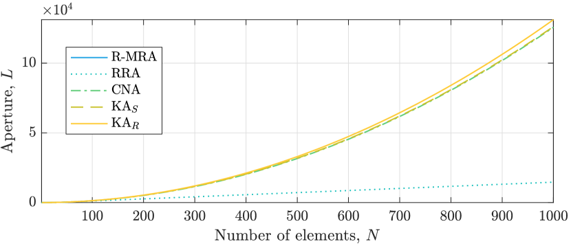
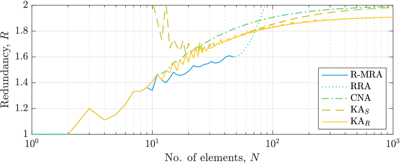
Fig. 7 shows the number of unit spacings $S(1)$ as a function of $N$ . In general, $S(1)$ increases linearly with $N$ , and the KA_R has the smallest rate of growth. The two exceptions are the KA_S and RRA, which have a constant $S(1)$ . However, unlike the RRA, the redundancy of the KA_S is bounded (cf. Fig. 6). As discussed in Section II-C3, the number of unit spacings $S(1)$ may be used as a simplistic indicator of the robustness of the array to mutual coupling. Assessing the effects of coupling ultimately requires actual measurements of the array response, or simulations using an electromagnetic model for the antenna and mounting platform [64, 65, 66, 67]. A detailed study of mutual coupling is therefore beyond the scope of this paper.

Obviously, many other important figures of merit are omitted here for brevity of presentation. For example, fragility and the achievable beampattern are natural criteria for array design or performance evaluation. Fragility quantifies the sensitivity of the co-array to physical sensor failures [68]. The array configurations studied in this paper only have essential sensors, and therefore high fragility, since the difference (and sum) co-array ceases to be contiguous if a sensor is removed. This is the cost of low redundancy. The beampattern is of interest in applications employing linear processing¹⁰¹⁰10For exceptions where the beampattern is also relevant when employing non-linear processing, see, e.g., [7, 69].. For example, in adaptive beamforming, the one-way (transmit or receive) beampattern is critical, whereas in active imaging, the two-way (combined transmit and receive) beampattern is more relevant. Although the one-way beampattern of a sparse array generally exhibits high sidelobes, a wide range of two-way beampatterns may be achieved using one [15] or several [3, 70] transmissions and receptions. The arrays discussed in this paper can achieve the same effective beampattern as the ULA of equivalent aperture by employing multiple transmissions and receptions.

VI-B Active sensing performance

The estimation of the angles and scattering coefficients from (1) can be formulated as an on-grid sparse support recovery problem, similarly to the passive sensing case described in [71]. In particular, let $\{\tilde{\varphi}_{i}\}_{i=1}^{V}$ denote a set of $V\gg K$ discretized angles. The task then becomes to solve

\displaystyle\underset{\bm{\bar{\gamma}}\in\mathbb{C}^{V}}{\text{minimize}}

\displaystyle\ \|\bm{x}-(\bm{\tilde{A}}\odot\bm{\tilde{A}})\bm{\tilde{\gamma}}\|_{2}^{2}\ \text{subject to}\ \|\bm{\tilde{\gamma}}\|_{0}=K,

(P6)

where $\bm{\tilde{A}}\in\mathbb{C}^{N\times V}$ is the known steering matrix sampled at the $V$ angles, and $\bm{\bar{\gamma}}\in\mathbb{C}^{V}$ the unknown sparse scattering coefficient vector. The sparsity of $\bm{\bar{\gamma}}$ is enforced by the $\ell_{0}$ pseudonorm $\|\bm{\tilde{\gamma}}\|_{0}\triangleq\sum_{i=1}^{V}\mathbbm{1}(\tilde{\gamma}_{i}\neq 0)$ , which enumerates the number of non-zero entries. Although (P6) is a non-convex optimization problem due to the $\ell_{0}$ pseudonorm, it can be approximately solved using Orthogonal Matching Pursuit (OMP). OMP is a greedy algorithm that iteratively finds the $k=1,2\ldots,K$ columns in the dictionary matrix $\bm{\tilde{A}}\odot\bm{\tilde{A}}$ whose linear combination best describes the data vector $\bm{x}$ in an $\ell_{2}$ sense. For details on the OMP algorithm, see [72], [73, p. 65].

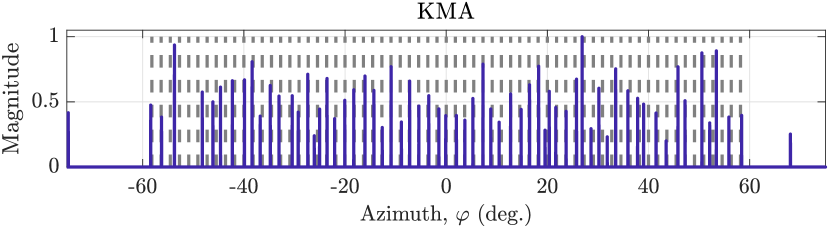
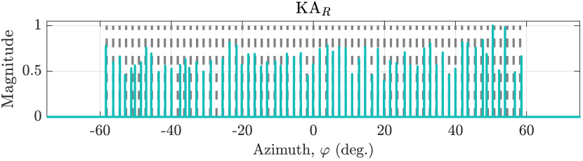
We now compare the active sensing performance of the KMA and KA_R using OMP. As demonstrated in Section VI-A, the KMA and KA_R achieve the lowest redundancy of the considered configurations with closed-form sensor positions. We consider $K=65$ scatterers with angles $\varphi_{k}$ uniformly spaced between $-60^{\circ}$ and $60^{\circ}$ . The scattering coefficients are spherically distributed complex-valued random variables, i.e., $\gamma_{k}=z_{k}/|z_{k}|$ , where $z\sim\mathcal{CN}(0,1)$ . We assume that the arrays consist of ideal omnidirectional sensors with unit inter-sensor spacing $\delta=1/2$ , such that the $(n,i)$ th entry of the sampled steering matrix is $\tilde{A}_{n,i}=\exp(j\pi d_{n}\sin\tilde{\varphi}_{i})$ . Angles $\{\tilde{\varphi}_{i}\}_{i=1}^{V}$ form a uniform grid of $V\!=\!10^{4}$ points between $-75^{\circ}$ and $75^{\circ}$ .

Fig. 8 shows that for a fixed aperture $L=70$ , the KA_R has $141/101\approx 40\%$ more contiguous DoFs than the KMA, at the expense of $21/17\approx 24\%$ more sensors¹¹¹¹11For reference, the R-MRA with aperture $L=70$ has $N=20$ sensors.. The KA_R can therefore resolve more scatterers than the KMA of equivalent aperture at little extra cost. This is illustrated in Fig. 9, which shows the noiseless spatial spectrum estimate produced by the OMP algorithm. Both arrays resolve more scatterers than sensors, although the KMA misses some scatterers and displays spurious peaks instead. The KA_R approximately resolves all scatterers due to its larger co-array. Fig. 9 shows the noisy OMP spectra when the SNR of the scene, defined as $K/\sigma^{2}$ , is $5$ dB. The spectrum degrades more severely in case of the KMA, partly because it has fewer physical sensors than the KA_R. These conclusions are validated by the empirical root-mean square error (RMSE) of the angle estimates, where $1000$ random realizations of the noise and scattering coefficients were used. In the noiseless case, the RMSE of the KMA is $8.6^{\circ}$ , whereas the KA_R achieves $4.2^{\circ}$ . In the noisy case the corresponding figures are $16.2^{\circ}$ (KMA) and $7.9^{\circ}$ (KA_R).

VII Conclusions and future work

This paper proposed a general symmetric sparse linear array design suitable for both active and passive sensing. We established a necessary and sufficient condition for the sum and difference co-array to be contiguous, and identified sufficient conditions that substantially simplify the array design. We studied two special cases in detail, the CNA and KA, both of which achieve a low redundancy and can be generated for any number of sensors $N$ . The KA achieves the lowest asymptotic redundancy among the considered array configurations. This also yields an upper bound on the redundancy of the R-MRA, whose exact value remains an open question. The upper bound may perhaps be tightened by novel sparse array designs suggested by the proposed array design methodology.

In future work, it would be of interest to characterize the redundancy of other symmetric arrays, including recursive/fractal arrays [13, 14, 15] that have a contiguous sum co-array. Another direction is investigating the advantages of symmetric arrays over co-array equivalent asymmetric arrays in more detail. This could further increase the relevance of the symmetric sparse array configurations studied in this paper.

Acknowledgment

The authors would like to thank Dr. Jukka Kohonen for bringing the Kløve basis to their attention and for the feedback on this manuscript, as well as for the many stimulating discussions regarding additive bases.

Appendix A Contiguous difference co-array of the KMA

We now show that the Kløve-Mossige array $\mathcal{G}$ in Definition 11 has a contiguous difference co-array. By symmetry of the difference co-array, it suffices to show that $\mathcal{G}-\mathcal{G}\supseteq\mathcal{C}\supseteq\{0:\max\mathcal{G}\}$ . We may easily verify that $\mathcal{G}-\mathcal{G}\supseteq\mathcal{C}$ holds for

	$\displaystyle\mathcal{C}$	$\displaystyle=(\mathcal{D}_{\text{CNA}}-\mathcal{D}_{\text{CNA}})\cup(\mathcal{D}_{3}-\mathcal{D}_{\text{CNA}}+2\max\mathcal{D}_{\text{CNA}}+1)$
		$\displaystyle\supseteq\{0:\max\mathcal{D}_{\text{CNA}}\}\cup(\mathcal{D}_{3}+\mathcal{D}_{\text{CNA}}+\max\mathcal{D}_{\text{CNA}}+1),$

where the second line follows from the fact that the CNA is symmetric and has a contiguous difference co-array. Consequently, $\mathcal{C}\supseteq\{0:\max\mathcal{G}\}$ holds if and only if

\displaystyle\mathcal{D}_{3}+\mathcal{D}_{\text{CNA}}=\{0:\max\mathcal{G}-\max\mathcal{D}_{\text{CNA}}-1\}.

Due to the periodicity of $\mathcal{D}_{3}$ , this condition simplifies to

\displaystyle\mathcal{D}_{4}+\mathcal{D}_{\text{CNA}}=\{0:\max\mathcal{D}_{\text{CNA}}+N_{1}^{2}\},

where $\mathcal{D}_{4}=\{0:N_{1}:N_{1}^{2}\}$ , and by Definition 10 we have

	$\displaystyle\mathcal{D}_{4}+\mathcal{D}_{\text{CNA}}=\{\mathcal{D}_{4}+\mathcal{D}_{1}\}$	$\displaystyle\cup\{\mathcal{D}_{4}+\mathcal{D}_{2}+N_{1}\}$
		$\displaystyle\cup\{\mathcal{D}_{4}+\mathcal{D}_{1}+N_{2}(N_{1}+1)\}.$

As $\mathcal{D}_{1}+\mathcal{D}_{4}=\{0:N_{1}(N_{1}+1)-1\}$ , it suffices to show that

\displaystyle\mathcal{D}_{4}+\mathcal{D}_{2}

\displaystyle\supseteq\{N_{1}^{2}:(N_{2}-1)(N_{1}+1)\}.

By Definitions 10 and 11, we have

	$\displaystyle\mathcal{D}_{4}+\mathcal{D}_{2}$	$\displaystyle=\{kN_{1}+l(N_{1}+1)\ \|\ k\in\{0:N_{1}\};l\in\{0:N_{2}-1\}\}$
		$\displaystyle=\{i(N_{1}+1)-k\ \|\ k\in\{0:N_{1}\};i-k\in\{0:N_{2}-1\}\}$
		$\displaystyle\supseteq\{i(N_{1}+1)-k\ \|\ k\in\{0:N_{1}\};i\in\{N_{1}:N_{2}-1\}\}$
		$\displaystyle\supseteq\{N_{1}^{2}:(N_{2}-1)(N_{1}+1)\},$

which implies that the difference co-array of $\mathcal{G}$ is contiguous.

Appendix B First hole in the sum co-array of the KMA

Let $\mathcal{G}$ denote the KMA in Definition 11. Furthermore, let $H\in\mathbb{N}$ , as defined in (3), be the first hole in $\mathcal{G}+\mathcal{G}$ . In the following, we show that

\displaystyle H=\begin{cases}2\max\mathcal{G}+1,&\text{if }N_{1}+N_{2}=1\\ h+1,&\text{if }N_{1}\geq 1\text{ and }N_{2}=1\\ h,&\text{otherwise},\end{cases}

where the non-negative integer $h$ is

	$\displaystyle h$	$\displaystyle=\max\mathcal{G}+\max\mathcal{D}_{\text{CNA}}+1$
		$\displaystyle=N_{3}(\max\mathcal{D}_{\text{CNA}}+1+N_{1}^{2})+2\max\mathcal{D}_{\text{CNA}}+1.$		(26)

The first case, which we only briefly mention here, follows trivially from the fact that $\mathcal{G}$ degenerates to the ULA when either $N_{1}=0$ and $N_{2}=1$ , or $N_{1}=1$ and $N_{2}=0$ . We prove the latter two cases by contradiction, i.e., by showing that $h+1\in\mathcal{G}+\mathcal{G}$ , respectively $h\in\mathcal{G}+\mathcal{G}$ , leads to an impossibility. Verifying that indeed $\mathcal{G}+\mathcal{G}\supseteq\{0:h\}$ , respectively $\mathcal{G}+\mathcal{G}\supseteq\{0:h-1\}$ , is left as an exercise for the interested reader.

We start by explicitly writing the sum co-array of $\mathcal{G}$ as

	$\displaystyle\mathcal{G}+\mathcal{G}=(\mathcal{D}_{\text{CNA}}+\mathcal{D}_{\text{CNA}})$	$\displaystyle\cup(\mathcal{D}_{\text{CNA}}+\mathcal{D}_{3}+2\max\mathcal{D}_{\text{CNA}}+1)$
		$\displaystyle\cup(\mathcal{D}_{3}+\mathcal{D}_{3}+4\max\mathcal{D}_{\text{CNA}}+2).$

Note that the CNA has a contiguous sum co-array, that is,

\displaystyle\mathcal{D}_{\text{CNA}}+\mathcal{D}_{\text{CNA}}=\{0:2\max\mathcal{D}_{\text{CNA}}\}.

Furthermore, it was shown in Appendix A that

\displaystyle\mathcal{D}_{\text{CNA}}+\mathcal{D}_{3}+2\max\mathcal{D}_{\text{CNA}}+1=\{2\max\mathcal{D}_{\text{CNA}}+1:h-1\}.

Consequently, $h\in\mathcal{G}+\mathcal{G}$ holds if and only if

\displaystyle h\in\mathcal{D}_{3}+\mathcal{D}_{3}+4\max\mathcal{D}_{\text{CNA}}+2.

By Definition 11, there must therefore exist non-negative integers $k\in\{0:2N_{1}\}$ and $l\in\{0:2(N_{3}-1)\}$ such that

\displaystyle h\!=\!kN_{1}+l(\max\mathcal{D}_{\text{CNA}}+1+N_{1}^{2})+4\max\mathcal{D}_{\text{CNA}}+2.

(27)

Substituting (26) into (27) and rearranging the terms yields

\displaystyle(N_{3}-l)(\max\mathcal{D}_{\text{CNA}}+1+N_{1}^{2})=2\max\mathcal{D}_{\text{CNA}}+1+kN_{1}.

Since $k\in\{0:2N_{1}\}$ , the following inequality must hold:

\displaystyle\frac{2\max\mathcal{D}_{\text{CNA}}+1}{N_{1}^{2}+\max\mathcal{D}_{\text{CNA}}+1}\leq N_{3}-l\leq\frac{2N_{1}^{2}+2\max\mathcal{D}_{\text{CNA}}+1}{N_{1}^{2}+\max\mathcal{D}_{\text{CNA}}+1}.

This reduces to $0<N_{3}-l<2$ , or more conveniently, $N_{3}-l=1$ , since $N_{3}-l$ is an integer. Consequently, we have

\displaystyle N_{1}(N_{1}-k)=\max\mathcal{D}_{\text{CNA}},

(28)

where $\max\mathcal{D}_{\text{CNA}}\geq 0$ leads to $N_{1}-k\in\{0:N_{1}\}$ . Substituting $\max\mathcal{D}_{\text{CNA}}=L$ in (12) into (28) yields

\displaystyle N_{1}-k=N_{2}+1+\frac{N_{2}-1}{N_{1}}.

(29)

Combined with $N_{1}-k\leq N_{1}$ , this implies that

\displaystyle N_{1}\geq\frac{N_{2}+1+\sqrt{(N_{2}+1)^{2}+4(N_{2}-1)}}{2}\geq N_{2}+1,

since $N_{1},N_{2}\geq 1$ . We identify the following two cases:

i)

If $N_{2}=1$ , then (29) yields that $N_{1}-k=2$ , implying that $H>h$ . However, it is straightforward to verify that $H=h+1$ from the fact that when $h$ is replaced by $h+1$ in (27), no integer-valued $N_{1}\geq 2$ satisfies the equation.
ii)

If $N_{2}\geq 2$ , then $N_{1}\leq N_{2}-1$ follows from (29), since $(N_{2}-1)/N_{1}$ must be an integer. This leads to a contradiction, since both $N_{1}\geq N_{2}+1$ and $N_{1}\leq N_{2}-1$ cannot hold simultaneously. Consequently, $H=h$ holds.

Finally, $H=h$ also holds when $N_{1}=0$ and $N_{2}\geq 2$ , or $N_{1}\geq 2$ and $N_{2}=0$ , since $\mathcal{G}$ degenerates into the NA in this case. This covers all of the possible values of $H$ .

References

[1] H. L. Van Trees, Optimum Array Processing, Part IV of Detection, Estimation, and Modulation Theory. Wiley-Interscience, 2002.
[2] R. A. Haubrich, “Array design,” Bulletin of the Seismological Society of America, vol. 58, no. 3, pp. 977–991, 1968.
[3] R. T. Hoctor and S. A. Kassam, “The unifying role of the coarray in aperture synthesis for coherent and incoherent imaging,” Proceedings of the IEEE, vol. 78, no. 4, pp. 735–752, Apr 1990.
[4] A. Koochakzadeh and P. Pal, “Cramér-Rao bounds for underdetermined source localization,” IEEE Signal Processing Letters, vol. 23, no. 7, pp. 919–923, July 2016.
[5] M. Wang and A. Nehorai, “Coarrays, MUSIC, and the Cramér-Rao bound,” IEEE Transactions on Signal Processing, vol. 65, no. 4, pp. 933–946, Feb 2017.
[6] C. L. Liu and P. P. Vaidyanathan, “Cramér-Rao bounds for coprime and other sparse arrays, which find more sources than sensors,” Digital Signal Processing, vol. 61, pp. 43 – 61, Feb 2017.
[7] P. Pal and P. P. Vaidyanathan, “Nested arrays: A novel approach to array processing with enhanced degrees of freedom,” IEEE Transactions on Signal Processing, vol. 58, no. 8, pp. 4167–4181, Aug 2010.
[8] C. L. Liu and P. P. Vaidyanathan, “Remarks on the spatial smoothing step in coarray MUSIC,” IEEE Signal Processing Letters, vol. 22, no. 9, pp. 1438–1442, Sep. 2015.
[9] A. Moffet, “Minimum-redundancy linear arrays,” IEEE Transactions on Antennas and Propagation, vol. 16, no. 2, pp. 172–175, Mar 1968.
[10] R. T. Hoctor and S. A. Kassam, “Array redundancy for active line arrays,” IEEE Transactions on Image Processing, vol. 5, no. 7, pp. 1179–1183, Jul 1996.
[11] M. Ishiguro, “Minimum redundancy linear arrays for a large number of antennas,” Radio Science, vol. 15, no. 6, pp. 1163–1170, 1980.
[12] C. L. Liu and P. P. Vaidyanathan, “Maximally economic sparse arrays and Cantor arrays,” in Seventh IEEE International Workshop on Computational Advances in Multi-Sensor Adaptive Processing, CAMSAP, Dec 2017, pp. 1–5.
[13] M. Yang, A. M. Haimovich, X. Yuan, L. Sun, and B. Chen, “A unified array geometry composed of multiple identical subarrays with hole-free difference coarrays for underdetermined doa estimation,” IEEE Access, vol. 6, pp. 14 238–14 254, 2018.
[14] R. Cohen and Y. C. Eldar, “Sparse fractal array design with increased degrees of freedom,” in IEEE International Conference on Acoustics, Speech and Signal Processing, ICASSP 2019, May 2019, pp. 4195–4199.
[15] ——, “Sparse array design via fractal geometries,” IEEE Transactions on Signal Processing, vol. 68, pp. 4797–4812, 2020.
[16] R. L. Haupt, “Thinned arrays using genetic algorithms,” IEEE Transactions on Antennas and Propagation, vol. 42, no. 7, pp. 993–999, 1994.
[17] B. Friedlander and A. J. Weiss, “Direction finding in the presence of mutual coupling,” IEEE Transactions on Antennas and Propagation, vol. 39, no. 3, pp. 273–284, Mar 1991.
[18] G. Xu, R. H. I. Roy, and T. Kailath, “Detection of number of sources via exploitation of centro-symmetry property,” IEEE Transactions on Signal processing, vol. 42, no. 1, pp. 102–112, 1994.
[19] R. Roy and T. Kailath, “ESPRIT — Estimation of signal parameters via rotational invariance techniques,” IEEE Transactions on Acoustics, Speech, and Signal Processing, vol. 37, no. 7, pp. 984–995, Jul 1989.
[20] A. L. Swindlehurst, B. Ottersten, R. Roy, and T. Kailath, “Multiple invariance ESPRIT,” IEEE Transactions on Signal Processing, vol. 40, no. 4, pp. 867–881, 1992.
[21] F. Gao and A. B. Gershman, “A generalized ESPRIT approach to direction-of-arrival estimation,” IEEE Signal Processing Letters, vol. 12, no. 3, pp. 254–257, 2005.
[22] B. Wang, Y. Zhao, and J. Liu, “Mixed-order music algorithm for localization of far-field and near-field sources,” IEEE Signal Processing Letters, vol. 20, no. 4, pp. 311–314, 2013.
[23] B. Wichmann, “A note on restricted difference bases,” Journal of the London Mathematical Society, vol. s1-38, no. 1, pp. 465–466, 1963.
[24] D. Pearson, S. U. Pillai, and Y. Lee, “An algorithm for near-optimal placement of sensor elements,” IEEE Transactions on Information Theory, vol. 36, no. 6, pp. 1280–1284, Nov 1990.
[25] D. A. Linebarger, I. H. Sudborough, and I. G. Tollis, “Difference bases and sparse sensor arrays,” IEEE Transactions on Information Theory, vol. 39, no. 2, pp. 716–721, Mar 1993.
[26] P. P. Vaidyanathan and P. Pal, “Sparse sensing with co-prime samplers and arrays,” IEEE Transactions on Signal Processing, vol. 59, no. 2, pp. 573–586, Feb 2011.
[27] C. L. Liu and P. P. Vaidyanathan, “Super nested arrays: Linear sparse arrays with reduced mutual coupling – Part I: Fundamentals,” IEEE Transactions on Signal Processing, vol. 64, no. 15, pp. 3997–4012, Aug 2016.
[28] C. Liu and P. P. Vaidyanathan, “Super nested arrays: Linear sparse arrays with reduced mutual coupling – Part II: High-order extensions,” IEEE Transactions on Signal Processing, vol. 64, no. 16, pp. 4203–4217, 2016.
[29] R. T. Hoctor and S. A. Kassam, “High resolution coherent source location using transmit/receive arrays,” IEEE Transactions on Image Processing, vol. 1, no. 1, pp. 88–100, Jan 1992.
[30] F. Ahmad, G. J. Frazer, S. A. Kassam, and M. G. Amin, “Design and implementation of near-field, wideband synthetic aperture beamformers,” IEEE Transactions on Aerospace and Electronic Systems, vol. 40, no. 1, pp. 206–220, Jan 2004.
[31] R. Rajamäki and V. Koivunen, “Sparse linear nested array for active sensing,” in 25th European Signal Processing Conference (EUSIPCO 2017), Kos, Greece, August 2017.
[32] ——, “Symmetric sparse linear array for active imaging,” in Tenth IEEE Sensor Array and Multichannel Signal Processing Workshop (SAM), Sheffield, UK, July 2018, pp. 46–50.
[33] ——, “Sparse low-redundancy linear array with uniform sum co-array,” in IEEE International Conference on Acoustics, Speech and Signal Processing, ICASSP 2020, Barcelona, Spain, May 2020, pp. 4592–4596.
[34] C. L. Liu and P. P. Vaidyanathan, “Super nested arrays: sparse arrays with less mutual coupling than nested arrays,” in IEEE International Conference on Acoustics, Speech, and Signal Processing, ICASSP 2016., Mar 2016.
[35] Z. Zheng, W. Wang, Y. Kong, and Y. D. Zhang, “MISC array: A new sparse array design achieving increased degrees of freedom and reduced mutual coupling effect,” IEEE Transactions on Signal Processing, vol. 67, no. 7, pp. 1728–1741, April 2019.
[36] S. Mossige, “Algorithms for computing the h-range of the postage stamp problem,” Mathematics of Computation, vol. 36, no. 154, pp. 575–582, 1981.
[37] H. Rohrbach, “Ein Beitrag zur additiven Zahlentheorie,” Mathematische Zeitschrift, vol. 42, no. 1, pp. 1–30, 1937.
[38] T. Kløve, “A class of symmetric 2-bases,” Mathematica Scandinavica, vol. 47, no. 2, pp. 177–180, 1981.
[39] J. Li and P. Stoica, “MIMO radar with colocated antennas,” IEEE Signal Processing Magazine, vol. 24, no. 5, pp. 106–114, Sep. 2007.
[40] E. BouDaher, F. Ahmad, and M. G. Amin, “Sparsity-based direction finding of coherent and uncorrelated targets using active nonuniform arrays,” IEEE Signal Processing Letters, vol. 22, no. 10, pp. 1628–1632, Oct 2015.
[41] C.-Y. Chen and P. P. Vaidyanathan, “Minimum redundancy MIMO radars,” in IEEE International Symposium on Circuits and Systems (ISCAS 2008), May 2008, pp. 45–48.
[42] C. C. Weng and P. P. Vaidyanathan, “Nonuniform sparse array design for active sensing,” in 45th Asilomar Conference on Signals, Systems and Computers, Nov 2011, pp. 1062–1066.
[43] X. Wang, Z. Chen, S. Ren, and S. Cao, “Doa estimation based on the difference and sum coarray for coprime arrays,” Digital Signal Processing, vol. 69, pp. 22 – 31, 2017.
[44] W. Si, F. Zeng, C. Zhang, and Z. Peng, “Improved coprime arrays with reduced mutual coupling based on the concept of difference and sum coarray,” IEEE Access, vol. 7, pp. 66 251–66 262, 2019.
[45] R. Rajamäki and V. Koivunen, “Sparse active rectangular array with few closely spaced elements,” IEEE Signal Processing Letters, vol. 25, no. 12, pp. 1820–1824, Dec 2018.
[46] ——, “Comparison of sparse sensor array configurations with constrained aperture for passive sensing,” in IEEE Radar Conference (RadarConf 2017), May 2017, pp. 0797–0802.
[47] E. BouDaher, F. Ahmad, M. G. Amin, and A. Hoorfar, “Mutual coupling effect and compensation in non-uniform arrays for direction-of-arrival estimation,” Digital Signal Processing, vol. 61, pp. 3–14, 2017.
[48] C. L. Liu and P. P. Vaidyanathan, “Hourglass arrays and other novel 2-d sparse arrays with reduced mutual coupling,” IEEE Transactions on Signal Processing, vol. 65, no. 13, pp. 3369–3383, July 2017.
[49] C. A. Balanis, Antenna theory: analysis and design, 4th ed. John Wiley & sons, 2016.
[50] J. Kohonen and J. Corander, “Addition chains meet postage stamps: reducing the number of multiplications,” Journal of Integer Sequences, vol. 17, no. 3, pp. 14–3, 2014.
[51] J. Kohonen, “A meet-in-the-middle algorithm for finding extremal restricted additive 2-bases,” Journal of Integer Sequences, vol. 17, no. 6, 2014.
[52] J. Riddell and C. Chan, “Some extremal 2-bases,” Mathematics of Computation, vol. 32, no. 142, pp. 630–634, 1978.
[53] J. Leech, “On the representation of $1,2,\dots,n$ by differences,” Journal of the London Mathematical Society, vol. s1-31, no. 2, pp. 160–169, 1956.
[54] J. Kohonen, “Early pruning in the restricted postage stamp problem,” arXiv preprint arXiv:1503.03416, 2015.
[55] S. Shakeri, D. D. Ariananda, and G. Leus, “Direction of arrival estimation using sparse ruler array design,” in IEEE 13th International Workshop on Signal Processing Advances in Wireless Communications, SPAWC 2012, June 2012, pp. 525–529.
[56] G. Yu, “A new upper bound for finite additive h-bases,” Journal of Number Theory, vol. 156, pp. 95 – 104, 2015.
[57] J. Kohonen, “An improved lower bound for finite additive 2-bases,” Journal of Number Theory, vol. 174, pp. 518 – 524, 2017.
[58] G. Yu, “Upper bounds for finite additive 2-bases,” Proceedings of the American Mathematical Society, vol. 137, no. 1, pp. 11–18, 2009.
[59] J. Kohonen, “Exact inference algorithms and their optimization in bayesian clustering,” Ph.D. dissertation, University of Helsinki, 2015.
[60] D. H. Werner and S. Ganguly, “An overview of fractal antenna engineering research,” IEEE Antennas and Propagation Magazine, vol. 45, no. 1, pp. 38–57, 2003.
[61] C. Liu and P. P. Vaidyanathan, “Optimizing minimum redundancy arrays for robustness,” in 52nd Asilomar Conference on Signals, Systems, and Computers, 2018, pp. 79–83.
[62] G. S. Bloom and S. W. Golomb, “Applications of numbered undirected graphs,” Proceedings of the IEEE, vol. 65, no. 4, pp. 562–570, April 1977.
[63] E. Vertatschitsch and S. Haykin, “Nonredundant arrays,” Proceedings of the IEEE, vol. 74, no. 1, pp. 217–217, 1986.
[64] J. L. Allen and B. L. Diamond, “Mutual coupling in array antennas,” Massachusetts Institute Of Technology Lexington Lincoln Lab, Tech. Rep. 424, 1966.
[65] J. Rubio, J. F. Izquierdo, and J. Córcoles, “Mutual coupling compensation matrices for transmitting and receiving arrays,” IEEE Transactions on Antennas and Propagation, vol. 63, no. 2, pp. 839–843, Feb 2015.
[66] C. Craeye and D. González-Ovejero, “A review on array mutual coupling analysis,” Radio Science, vol. 46, no. 2, 2011.
[67] B. Friedlander, “The extended manifold for antenna arrays,” IEEE Transactions on Signal Processing, vol. 68, pp. 493–502, 2020.
[68] C. Liu and P. P. Vaidyanathan, “Robustness of difference coarrays of sparse arrays to sensor failures—part I: A theory motivated by coarray MUSIC,” IEEE Transactions on Signal Processing, vol. 67, no. 12, pp. 3213–3226, 2019.
[69] R. Cohen and Y. C. Eldar, “Sparse convolutional beamforming for ultrasound imaging,” IEEE Transactions on Ultrasonics, Ferroelectrics, and Frequency Control, vol. 65, no. 12, pp. 2390–2406, Dec 2018.
[70] R. J. Kozick and S. A. Kassam, “Linear imaging with sensor arrays on convex polygonal boundaries,” IEEE Transactions on Systems, Man, and Cybernetics, vol. 21, no. 5, pp. 1155–1166, Sep 1991.
[71] P. Pal and P. P. Vaidyanathan, “Pushing the limits of sparse support recovery using correlation information,” IEEE Transactions on Signal Processing, vol. 63, no. 3, pp. 711–726, Feb 2015.
[72] J. A. Tropp, “Greed is good: algorithmic results for sparse approximation,” IEEE Transactions on Information Theory, vol. 50, no. 10, pp. 2231–2242, 2004.
[73] S. Foucart and H. Rauhut, A Mathematical Introduction to Compressive Sensing. Birkhäuser, 2013.

	$\displaystyle\mathcal{D}_{4}+\mathcal{D}_{2}$	$\displaystyle=\{kN_{1}+l(N_{1}+1)\ \|\ k\in\{0:N_{1}\};l\in\{0:N_{2}-1\}\}$
		$\displaystyle=\{i(N_{1}+1)-k\ \|\ k\in\{0:N_{1}\};i-k\in\{0:N_{2}-1\}\}$
		$\displaystyle\supseteq\{i(N_{1}+1)-k\ \|\ k\in\{0:N_{1}\};i\in\{N_{1}:N_{2}-1\}\}$
		$\displaystyle\supseteq\{N_{1}^{2}:(N_{2}-1)(N_{1}+1)\},$

Sparse Symmetric Linear Arrays with Low Redundancy and a Contiguous Sum Co-Array

Abstract

Index Terms:

I Introduction

I-A Contributions and organization

I-B Notation

II Preliminaries

II-A Signal model

II-B Sum co-array

Definition 1 (Sum co-array).

Definition 2 (Contiguous sum co-array).

II-C Array figures of merit

II-C1 Degrees of freedom (DoF).

Definition 3 (Number of contiguous DoFs).

II-C2 Redundancy,

Definition 4 (Redundancy).

II-C3 The dd-spacing multiplicity,

Definition 5 (dd-spacing multiplicity [45]).

II-C4 Asymptotic and relative quantities.

III Minimum-Redundancy Array

Definition 6 (Minimum-redundancy array (MRA)).

III-A Key properties

Lemma 1 (Necessary sensors).

Proof.

Corollary 1 (Perfect arrays).

Proof.

Theorem 1 (Asymptotic redundancy of MRA [56, 57, 38, 58]).

Proof.

III-B Unique solution with fewest closely spaced sensors

III-C Symmetry and the Reduced Redundancy Array

Definition 7 (Reduced redundancy array (RRA) [10]).

IV Symmetric array — general design and conditions for contiguous co-array

Definition 8 (Symmetric array with generator 𝒢\mathcal{G} (S-𝒢\mathcal{G})).

IV-A Necessary and sufficient conditions for contiguous co-array

Theorem 2 (Conditions for contiguous co-array).

Proof.

IV-B Sufficient conditions for contiguous co-array

Corollary 2 (Sufficient conditions for (C1)).

Proof.

Corollary 3 (Sufficient conditions for (C2)).

Proof.

V Low-redundancy symmetric array designs using parametric generators

V-A Symmetric Nested Array (S-NA)

Definition 9 (Symmetric Nested Array (S-NA)).

V-A1 Concatenated Nested Array (CNA)

Definition 10 (Concatenated Nested Array (CNA) [31]).

V-A2 Minimum-redundancy solution

Proposition 1.

Proof.

Lemma 2.

Proof.

Theorem 3 (Minimum-redundancy parameters of CNA).

Proof.

Corollary 4 (Properties of minimum-redundancy CNA).

Proof.

V-B Symmetric Kløve-Mossige array (S-KMA)

Definition 11 (Symmetric Kløve-Mossige Array (S-KMA)).

V-B1 Kløve array

Definition 12 (Kløve array (KA) [38]).

V-B2 Minimum-redundancy solution

Theorem 4 (Minimum-redundancy parameters of KA).

Proof.

Corollary 5 (Properties of minimum-redundancy KA).

Proof.

Proposition 2 (Asymptotic redundancy of KA [38]).

Proof.

V-B3 Polynomial time grid search

Proposition 3 (Cardinality of feasible set in (P5)).

Proof.

V-C Other generator choices

VI Performance evaluation of array designs

VI-A Comparison of array figures of merit

VI-A1 Non-contiguous sum co-array

VI-A2 Contiguous sum co-array

VI-B Active sensing performance

VII Conclusions and future work

Acknowledgment

Appendix A Contiguous difference co-array of the KMA

Appendix B First hole in the sum co-array of the KMA

References

II-C3 The $d$ -spacing multiplicity,

Definition 5 ( $d$ -spacing multiplicity [45]).

Definition 8 (Symmetric array with generator $\mathcal{G}$ (S- $\mathcal{G}$ )).