Some obstructions on the subgroups of the Brin-Thompson groups and a selection of twisted Brin-Thompson groups

We first introduce the group $V$ briefly as follows.

From the definition, we see that the interval $[0,1]$ is divided so that the subintervals are only in the form $\big{[}\frac{\ell}{2^{k}},\frac{\ell+1}{2^{k}}\big{]}$ where $\ell+1\leq 2^{k}$ and $k,\ell\in\mathbb{N}\cup\{0\}$. We call such intervals dyadic intervals. The dyadic intervals in the unit interval $[0,1]$ can be identified with middle third Cantor set $C,$ the set obtained by iteratively deleting the open middle third from the unit interval $I=[0,1],$ in a way that we associate the dyadic breakpoints with the open middle third part in $C$ which is cut out. By the above identification, the group $V$ can be regarded as a group acting on the Cantor set $C$ which is an alternative interpretation of the boundary of the rooted infinite binary tree denoted by $\partial(\mathcal{T}_{\infty}).$ The group $V$ can then be interpreted as a group acting on the infinite binary tree by partial automorphism of the rooted infinite binary tree $\mathcal{T}_{\infty}$ which resembles the definition give by Funar and Sergiescu’s description in [14].

Now we want to generalise the group $V$ to some higher dimensional families. We consider the “dyadic blocks” which are called “patterns” in Brin’s definition and called “dyadic brick” in Belk, Matucci and Zaremskiy’s definition [6]. The dyadic blocks can be seen as the generalisations of the dyadic intervals.

We first follow Brin’s original description [9] and zoom into the case of $2V.$ We take the Cantor set $C$ as described in the previous paragraph and identify the points of $C$ with the set of all binary words in $\{0,1\}.$ We view $C\times C$ as a subset of the unit square $I^{2}=[0,1]\times[0,1].$

A $2$-dyadic block (which are called “pattern” in Brin’s original definition) is identified with $I^{2}$ having a finite set of the rectangles in it with pairwise disjoint, non-empty interiors, with sides parallel to the sides of $I^{2}$ and whose union is all of $I^{2}.$ The trivial $2$-dyadic block is the square $I^{2}$ itself.

We denote this trivial $2$-dyadic blocks by $B(\epsilon,\epsilon)$ where $\epsilon$ represent the empty binary word and each of the rectangles inside $B(\epsilon,\epsilon)$ by $B(\omega_{0},\omega_{1})$ where $\omega_{0},\omega_{1}\in\{0,1\}^{\ast}$ are some binary words of finite length associated with the construction below.

Define inductively general $2$-dyadic blocks by dividing $I^{2}$ into rectangles with horizontal or vertical lines each at one step such that the sides of the rectangles are the finitely many dyadically subdivided intervals.

When we divide $I^{2}$ by a horizontal line segment, we denote the rectangle on the top by $B(\epsilon,0)$ and the rectangle at the bottom by $B(\epsilon,1).$ Here the first coordinate in this representation of the dyadic blocks somehow corresponding to the subdivision in the horizontal part by dyadic line segments. The notation for the rectangles constructed by the vertical subdivision are $B(0,\epsilon)$ and $B(1,\epsilon).$

Each rectangle $B(\cdot,\cdot)$ corresponds to a closed and open subset of $C\times C$ and $I^{2}$ corresponds to the union of the all the rectangles which is $C\times C.$ Here we assign to each rectangle whose union form $B(\epsilon,\epsilon),$ a number $i\in\mathbb{N}$ independent of the subdivision and denote the rectangle by $B_{i}(\cdot,\cdot).$

Now we associate the Cantor space $C^{2}$ with the dyadic block description as follows: take $\varphi_{i}=(\varphi_{i}(1),\varphi_{i}(2))$ where $\varphi_{i}(1)$ and $\varphi_{i}(2)$ are finite binary strings $\{0,1\}^{\ast}.$ We denote by

one of the rectangles in the subdivision and denote by $B(\varphi)=\{B_{i}(\varphi)\}$ the $2$-dyadic block with finitely many rectangles as disjoint subdivided regions associated to $\varphi$ where $i\in\{0,\cdots m-1\}$ and $m$ is the label of the rectangles in the $2$-dyadic blocks. $B(\varphi)$ is called the cone on $\varphi$ in Zaremsky’s definition [18] associated to $C^{2}$ by canonical homeomorphism

taking the pair $(\kappa(1),\kappa(2))$ to $(\varphi_{i}(1)\kappa(1),\varphi_{i}(2)\kappa(2))$ for all $i$ and $\kappa(1),\kappa(2)$ are some infinite strings in $C.$

For $B(\varphi)$ and $B(\psi)$, two labeled $2$-dyadic blocks with the same number of rectangles, we label the rectangles as mentioned above and then obtain a self-homeomorphism of $C\times C$ mapping each open or closed set in $C\times C$ associated with rectangles having the same labelings affinely.

The meaning of the word “affinely” here can be interpreted as “affine homotheties” of rectangles or, more precisely, affine maps preserving the horizontal and vertical directions: when we regard a trivial $2$-dyadic block $[0,1]\times[0,1]$ as a square embedded in the Euclidean plane $\mathbb{R}^{2}$ with vertices $(0,0)$, $(0,1)$, $(1,0)$ and $(1,1),$ then partitions defined above are the line segments embedded in the square with length $\frac{1}{2^{k}}$ for some integer $k.$

The rectangle $B_{i}(\varphi)$ maps to $B_{i}(\psi)$ affinely means that there is an affine linear transformation that maps every point $B_{i}(\varphi)$ in the source to every point in $B_{i}(\psi)$ in the target. We call these rectangles the sub $2$-dyadic blocks or subblocks in the rest of the paper.

This affine map can be regarded as a collection of prefix replacement maps taking each subblocks $\{B_{i}(\varphi(1),\varphi(2))\}$ in the source to each subblocks $\{B_{i}(\psi(1),\psi(2))\}$ in the target together with canonical homeomorphisms, they provide the self homeomorphisms we want, i.e.

The higher dimensional version of the groups $nV$ can be defined similarly. The group elements are acting on $C^{n}$ as prefix-replacement maps in [3, 1, 4].

We follow the definition from Belk et.al.[5, 18] to define the twisted version of the group $2V$ by introducing the twist homeomorphism induced by the group action. Let $G$ be a group acting on the set $\{1,2\}$ by permutation, i.e. $G\mapsto\mathfrak{S}_{2}$ where $\mathfrak{S}_{2}$ denotes the symmetric group of order $2.$ Take $\gamma_{j_{1}},\gamma_{j_{2}}\in G,$ define the basic twists induced by the action of $\gamma_{j_{i}}$ on $\{1,2\}$ to be

that maps each rectangle

to rectangles

taking subblocks

to

for $i\in\mathbb{N}.$ Then the twisted version of the self-homeomorphisms can be defined as follows,

This definition again can be generalised to $nV_{G}$ by considering the action of a group $G$ on larger sets with $n$ elements or even an infinite set.

Many of the known results on Brin-Thompson groups $nV$ are, somehow, motivated by the study on the embedding problems of the groups or finding out the structure of the conjugacy classes and the certralisers of the groups. It has been shown that this family of generalisation of Thompson’s groups has interesting and rich geometry: The groups $nV$ are proved to be simple, to be finitely presented [9] and more generally have finiteness property $FP_{\infty}$ [16]. They also contain many interesting classes of subgroups such as $RAAG$s, $RACG$s and many groups constructed from direct products and wreath products of infinite cyclic groups $\mathbb{Z}$ [2, 8].

Moreover, Brin-Thompson groups also contain a large class of the groups called the rational groups according to [3] which provide some indication on the “coarse” hyperbolic-type properties of the groups.

The isomorphism problem has been investigated by [7] with the result that, for any $n\neq m,$ $nV$ and $mV$ are not isomorphic. A selection of the results on the embedding problems and subgroup distortion are as follows: Some $RAAG$s and $RACG$s can be embedded into $nV,$ Bleak, Belk, Matucci; Kato [3, 15] while $\mathbb{Z}^{n+1}\ast\mathbb{Z}$ does not embed into $nV$[13]; When considering the wreath product instead of the directly product, we have $\mathbb{Z}^{n}\wr\mathbb{Z}^{n}$ embeds into $2V$; The groups $F,T,V$ are distorted in $2V.$

From a more combinatorial perspective, Belk, Bleak and Hyde [1] proved that these groups have solvable word problem, but unsolvable torsion problem which is provided as the first concrete examples of the groups described in Arzhantseva, Lafonts, Minasyanin [1].

In addition, as is mentioned previously, Belk and Matucci [6] have constructed and investigated the class of twisted Brin-Thompson groups and proved simplicity results and the finiteness properties for the class with some restrictions. A more recent paper by Zaremsky [18] provide more details on the motivation and relations to other problems. Some of the above results lead us to the following investigation on the torsion elements in $2V.$

Thompson’s group $F$ is torsion free while the groups $T,$ and $V$ have torsion elements, $T$ contains all the finite cyclic groups and $V$ has all finite groups inside it.

As is mentioned in the Introduction, Burillo, Cleary, Röver [11] provided a list of the obstructions for the subgroups of Thompson’s groups $V.$ One of properties that $V$ has, is the torsion local finiteness which provides some hints on what the torsion elements in $V$ should be like and should interact with other torsion elements. Torsion local finiteness of $V$ excludes infinite torsion subgroups such as Grigorchuck groups and provide an answer to the Burnside problems.

In addition, torsion local finiteness is a property that can be passed to subgroups, thus, we expect $2V$ (and even $nV$ for general positive integer $n$) to have the same property. We first state the definition of torsion locally finite as follows,

Inspired by the fact that torsion elements in $V$ can be represented by identical tree pairs, we consider one of the most obvious combinatorial representatives that a torsion element in $2V$ can be: an identical $2$-dyadic block pair.

For an identical $2$-dyadic block pair, we can obtain an identical rooted finite tree pair that correspond to the identical block pair depicted in Figure 5. Here, the fact that we can interchange the tree pairs and $2$-dyadic blocks pairs indicates that the torsion elements in the group $2V$ have similar dynamics as the ones in $V.$

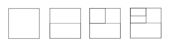
We describe more precisely how we obtain an identical tree pair from an identical dyadic block pair as follows: Since we define a 2-dyadic block inductively by adding horizontal and vertical line segments which are the partition line segments in $I^{2},$ we can naturally describe a partial order on these line segments, which is on the set of the horizontal and vertical dyadic line segments and the length of these line segments in the set form a monotonically decreasing sequence.

Nevertheless, there is one particular case that one needs to be careful: there is a dyadic block that can be produced by different sets of the partition lines and hence the two different set of the partition line segments have slight different partial order three line segments, but this difference is not going to have effect on partial order of other line segments in the set.

In Figure 6, the two sets of the partition line segments provide the same $2$-dyadic block, but the block on the left is partitioned by one vertical partition line segment with length $1$ first and then by two horizontal partition line segments with length $\frac{1}{2}$ from the left to the right, while the one on the right is partitioned by one horizontal partition line segment with length $1$ first and then two vertical partition line segments with length $\frac{1}{2}$ from the top to the bottom subblocks.

With the partial order defined, we can build rooted binary trees from dyadic blocks by associating $2$-carets (a vertex attached with two edges) to the partition line segments. The product of the unit interval $I^{2}$ corresponding to $C^{2}$ (also called the trivial pattern) can be associated to the root of a binary tree. We next attach a $2$-caret to the root, when we have either a horizontal or a vertical partition line segment in the dyadic block with length $1,$ then for the vertices on the other end of the two edges of the $2$-caret, we call them leaves of a $2$-caret, corresponding to the two subblocks after the partition.

We attach $2$-carets to the leaves corresponding to the previously constructed subblocks inductively according to the partial order of the partition line segments.

The partial order on the partition line segments also provides an order on how we are expanding the blocks which influences the partial ordering on the subblocks. In the case in Figure 6, the dyadic block on the left is first divided into two subblocks, the left and right subblocks, then the two subblocks are further divided into two subblocks, top and bottom each. while the dyadic block on the right is first subdivided into top and bottom subblocks and then left and right subblocks further. So there is a different “hierarchy” in the set of the dyadic blocks and subblocks.

Thus, we have associated an identical $2$-dyadic block pair with an identical rooted binary tree pair by the above construction.

This resembles the combinatorial properties of torsion elements and torsion subgroups in $V$ [12] that torsion elements can be represented by identical tree pairs and these pairs reveal the dynamics of the elements.

When we take an infinite set $\mathscr{S},$ the group $\mathscr{S}V_{G}$ will be more complicated regardless of the group action, thus, we first consider the non twisted case, then the group $\mathscr{S}V$ contains all of $\mathbb{N}V$ when $\mathscr{S}$ is a set of infinite order.

The group $SV$ considered in [9, 5] are subgroups of $\mathscr{S}V$ that can be regarded as some kind of “Arfinification” of the group $nV$ with some extra restrictions on the number of partitions and they includes all $nV$s as subgroups

Let $f\in\mathscr{S}V,$ then $f$ can be represented by $(B(\varphi),B(\psi))$ a pair of infinite dimensional blocks $[0,1]^{\mathbb{N}}$ (corresponding to the product of infinitely many Cantor sets $C^{\mathbb{N}}$) with dyadic subdivisions, with elementary expansions and collapses defined similarly. Moreover, there is still this partial order on partitioning the blocks. Then the group operation can be defined as the multiplication on blocks and the group structure follows.

Then Lemma 2.4 and Proposition 2.7 do not hold for the general $\mathscr{S}V$ any more, since, for instance, we have elements in $\mathscr{S}V$ that can be represented by identical pair having permutations of infinite order.

The latter condition in the if part in the preceeding Lemma indicate that there exists some more exotic torsion elements and we now closely look at some of these torsion elements in $SV$ for countable infinite set $S.$ We take an element $f\in\mathscr{S}V$ to have the identical block pair representation $(B(\varphi),B(\psi))$ such that the block pairs are constructed as follows:

for $i\in\mathbb{N}$ are two countable infinite sets where each block has infinite dimension. Take $\big{[}0,1\big{]}^{\mathbb{N}}$ to be $B(\epsilon,\epsilon,\cdots),$ we partition the first interval $\big{[}0,1]$ into half to obtain two subblocks $B(0,\epsilon,\cdots),$ and $B(1,\epsilon,\cdots).$ Next, we take the subblocks and subdivide the two subblocks $B(0,\epsilon,\cdots),$ $B(1,\epsilon,\cdots)$ into the following four blocks $B(0,0,\cdots),$ $B(0,1,\cdots)$ and $B(1,0,\cdots),$ $B(1,1,\cdots).$ For the next step, we take the last subblock $B(1,1,\cdots).$ and partition it to obtain $B(1,1,0,\cdots)$ and $B(1,1,1,\cdots).$ Then we take the last subblock $B(1,1,1,\cdots)$ and repeat the process of partitioning the blocks all over again and we will ultimately obtain an infinite sequence of the partitioned subblocks whose union form $\big{[}0,1\big{]}^{\mathbb{N}}.$ Here we can associate the partitions ( which are the dyadic subblocks) to an infinite binary tree according to the order of the partitions as described in Subsection 2.2. The identical block pairs $(B(\varphi),B(\psi))$ can now be represented by a pair of infinite binary trees. We now label the subblocks as follows,

References

- [1] James Belk and Collin Bleak. Some undecidability results for asynchronous transducers and the brin-thompson group . Transactions of the American Mathematical Society, 369(5):3157–3172, May 2017. Funding: partial support by UK EPSRC grant EP/H011978/1 (CB).
- [2] James Belk, Collin Bleak, and Francesco Matucci. Embedding Right-angled artin groups into Brin Thompson groups. Mathematical Proceedings of the Cambridge Philosophical Society, 169(2):225–229, apr 2019.
- [3] James Belk, James Hyde, and Francesco Matucci. On the asynchronous rational group. Groups, Geometry, and Dynamics, 13(4):1271–1284, sep 2019.
- [4] James Belk, James Hyde, and Francesco Matucci. Embeddings of into some finitely presented groups. arXiv preprint math:2005.02036., 2020.
- [5] James Belk and Matthew C. B. Zaremsky. Twisted brin-thompson groups. 01 2020.
- [6] James Belk and Matthew C. B. Zaremsky. Twisted Brin-Thompson groups. arXiv preprint math: 2001.04579, 2021.
- [7] Collin Bleak, Casey Donoven, and Julius Jonušas. Some isomorphism results for Thompson-like groups . Israel Journal of Mathematics, 222(1):1–19, oct 2017.
- [8] Collin Bleak, Francesco Matucci, and Max Neunhöffer. Embeddings into Thompson’s group V and coCF groups. Journal of the London Mathematical Society, 94(2):583–597, jul 2016.
- [9] Matthew G. Brin. Higher dimensional Thompson groups. Geom. Dedicata, 108:163–192, 2004.
- [10] José Burillo and Sean Cleary. Metric properties of higher-dimensional Thompson’s groups. Pacific Journal of Mathematics, 248(1):49–62, Oct 2010.
- [11] José Burillo, Sean Cleary, and Claas E. Röver. Obstructions for subgroups of Thompson’s group . In Geometric and cohomological group theory, volume 444 of London Math. Soc. Lecture Note Ser., pages 1–4. Cambridge Univ. Press, Cambridge, 2018.
- [12] José Burillo, Sean Cleary, Melanie Stein, and Jennifer Taback. Combinatorial and metric properties of Thompson’s group . Trans. Amer. Math. Soc., 361(2):631–652, 2009.
- [13] Nathan Corwin. Embedding and nonembedding results for r. thompson’s group v and related groups. Dissertations, Theses, and Student Research Papers in Mathematics, 2013.
- [14] Louis Funar, Christophe Kapoudjian, and Vlad Sergiescu. Asymptotically rigid mapping class groups and Thompson’s groups. In Handbook of Teichmüller theory. Volume III, volume 17 of IRMA Lect. Math. Theor. Phys., pages 595–664. Eur. Math. Soc., Zürich, 2012.
- [15] Motoko Kato. Embeddings of right-angled artin groups into higher-dimensional thompson groups. Journal of Algebra and Its Applications, 17(08):1850159, jul 2018.
- [16] Marco Marschler. Finiteness properties of the Braided Thompson’s groups and the Brin-Thompson groups. 2015.
- [17] Claas E Röver. Subgroups of finitely presented simple groups. PhD Thesis, University of Oxford, UK, page 97, 1999.
- [18] Matthew C. B. Zaremsky. A taste of twisted brin-thompson groups. 01 2022.