Solution approaches for evaporation-driven density instabilities in a slab of saturated porous media

We consider an isotropic, uniform slab of a porous medium which is mapped to the semi-infinite domain $\Omega_{H}=\{(x,y,z)\in\mathbb{R}^{3}:0\leq z\leq H\}$, where $H$ is the height of the medium. The assumption that the entire domain is saturated allows us to model the problem with single-phase flow equations which enables the analytical treatment in the linear stability section 3 later. The following equations govern the behaviour of the described system when the Boussinesq approximation is employed:

	$$\displaystyle\nabla\cdot\mathbf{v}=0~{},$$		(1)
	$$\displaystyle\mathbf{v}=-\dfrac{K}{\mu}\bigl{(}\nabla p+\rho g\mathbf{e_{z}}\bigr{)}~{},$$		(2)
	$$\displaystyle\phi\partial_{t}c+\nabla\cdot\bigl{(}c\mathbf{v}\bigr{)}=D\nabla^{2}c~{}.$$		(3)

Here, $\mathbf{v}$ is the Darcy flux, $K$ is the scalar permeability, $\mu$ is the dynamic viscosity of water and $p$ is the pressure. Moreover, the fluid density $\rho$, gravitational acceleration $g$, porosity $\phi$, effective diffusion constant $D$ of salt in water, as well as the salt concentration $c$ appear in the equations.

The first equation (1) is the continuity equation under the Boussinesq approximation, which states that density differences of the fluid are small such that they can be neglected everywhere except when multiplied by the gravitational acceleration. The second equation (2) is Darcy’s law, the momentum equation describing fluid flow in porous media. Lastly, equation (3) is a convection-diffusion equation governing the salt concentration.

In this setting, we will neglect chemical reactions such as the precipitation of salt once the salinity exceeds the solubility limit. This means that the model together with the following investigations and results are only valid up to the solubility limit which is 359 gram of salt per liter [4] at 20 degrees Celsius and atmospheric pressure. We also disregard the effect of temperature variations since they play only a minor role for the stability of the boundary layer in comparison to salinity differences in the considered scenario [10]. Consequently, the third equation is coupled with Darcy’s law via the linear equation of state

$$\rho(c)=\rho_{0}\bigl{(}1+\gamma(c-c_{0})\bigr{)}~{},$$

(4)

which relates the water density only to the salinity $c$. In this equation, $\rho_{0}$ and $c_{0}$ are a reference density and salt concentration, and will be chosen as the initial density of the liquid and the initial salt concentration, respectively, which are both assumed constant in space. Also, $\gamma$ is the density expansion coefficient of water with increasing salinity.

In the investigated scenario, the laterally unbounded porous slab is coupled to an infinite reservoir of saline groundwater with concentration $c_{0}$ at the bottom. At the surface, water is evaporating, e.g. due to wind or the influence of the sun. This is modeled by a fixed evaporation rate $E$ as vertical velocity. In order to adhere to the continuity equation, reservoir water has to enter the porous medium from below at the same rate. Since salt does not leave the porous slab during the evaporation process, a no-flux condition is imposed on the salinity at the top of the medium. In mathematical form, the boundary conditions of the system under investigation are given by:

	$\displaystyle\mathbf{v}(x,y,z=0,t)=\mathbf{v}(x,y,z=H,t)=E\mathbf{e_{z}}~{},$		(5)
	$\displaystyle c(x,y,z=0,t)=c_{0},~{}\bigl{(}c\mathbf{v}-D\nabla c\bigr{)}\cdot\mathbf{e_{z}}\Big{|}_{z=H}=0~{}.$		(6)

As an initial condition, we assume that the salt is homogeneously distributed in the domain:

$$c(x,y,z,t=0)=c_{0}~{}.$$

(7)

Since $c$ is the only quantity whose time derivative appears in the equations, this initial condition is sufficient for the problem to be well-posed.

In order to quantitatively investigate the system, it is advantageous to introduce reference values for each physical variable to lower the number of parameters at play and make the equations dimensionless. We choose $D/E$ as the length scale as it relates the advective velocity - in this scenario the evaporation rate - to the diffusivity of salt and therefore is a ratio between the two prevalent transport mechanisms. Furthermore, the reference velocity is chosen as the gravitational velocity $K\rho_{0}gc_{0}\gamma/\mu$ and the reference time as $\phi D/E^{2}$. The dimensionless density and salinity are defined such that they are equal to zero at the starting time and track the deviation from the initial state as time goes on. The same approach is used for the pressure, which means that the initial hydrostatic pressure profile has to be subtracted from the actual pressure before the nondimensionalization takes place. Here, both these steps are done at once and the resulting definitions of the nondimensional quantities read:

$\hat{x},\hat{y},\hat{z}=x,y,z~{}\dfrac{E}{D}$ , $\hat{\mathbf{v}}=\mathbf{v}\dfrac{\mu}{K\rho_{0}gc_{0}\gamma}$ , $\hat{c}=\dfrac{c-c_{0}}{c_{0}}$ , $\hat{t}=t\dfrac{E^{2}}{\phi D}$ , $\hat{p}=\dfrac{\bigl{(}p-\rho_{0}gz\bigr{)}E}{D\rho_{0}gc_{0}\gamma}$ , $\hat{\rho}=\dfrac{\rho-\rho_{0}}{\rho_{0}c_{0}\gamma}$.

(8)

From now on, the variables with hat are the dimensionless counterparts of the original variables. Definition (8) yields dimensionless equations in a very convenient form:

	$$\displaystyle\hat{\nabla}\cdot\hat{\mathbf{v}}=0~{},$$		(9)
	$$\displaystyle\hat{\mathbf{v}}=-\bigl{(}\hat{\nabla}\hat{p}+\hat{c}~{}\mathbf{e_{z}}\bigr{)}~{},$$		(10)
	$$\displaystyle\partial_{\hat{t}}\hat{c}+\hat{\nabla}\cdot\bigl{(}\mathrm{Ra}~{}\hat{c}~{}\hat{\mathbf{v}}-\hat{\nabla}\hat{c}\bigr{)}=0~{}.$$		(11)

As $\hat{c}$ and $\hat{\rho}$ are equal to each other, the density term in Darcy’s law is simply replaced by the salinity. The Rayleigh number $\mathrm{Ra}$ in this context is defined as

$$\mathrm{Ra}=\dfrac{K\rho_{0}gc_{0}\gamma}{E\mu}~{},$$

(12)

which can be read as the quotient between the reference velocity as defined in equation (8) and the evaporation rate $E$. The dimensionless initial and boundary conditions are

$$\begin{gathered}\hat{c}(\hat{x},\hat{y},\hat{z},\hat{t}=0)=0~{},\\ \hat{\mathbf{v}}(\hat{x},\hat{y},\hat{z}=0,\hat{t})=\hat{\mathbf{v}}(\hat{x},\hat{y},\hat{z}=\alpha,\hat{t})=\dfrac{1}{\mathrm{Ra}}\mathbf{e_{z}}~{},\\ \hat{c}(\hat{x},\hat{y},\hat{z}=0,\hat{t})=0,~{}\bigl{(}\hat{c}+1-\partial_{\hat{z}}\hat{c}\bigr{)}\Big{|}_{\hat{z}=\alpha}=0~{},\end{gathered}$$

(13)

where $\alpha$ is the dimensionless height of the porous slab:

$$\alpha=\dfrac{HE}{D}~{}.$$

(14)

This quantity is an important characteristic of the problem as it quantifies to what degree diffusion is capable of smoothing out the salt concentration over the entire domain height while counteracting advection. As long as there is no convection and the flow velocity is equal to $E$, $\alpha$ also corresponds to the Péclet number. Generally, interesting values of $\alpha$ are in the range of $1-1000$ since the diffusion constant of salt in water is of the order $10^{-9}\,\nicefrac{\mathrm{m^{2}}}{\mathrm{s}}$ according to Moum et al. [17] and common evaporation rates are roughly $10^{-8}-10^{-9}\,\nicefrac{\mathrm{m}}{\mathrm{s}}$ depending on the specific ambient conditions [23]. Thus, for heights of $1-100\,\mathrm{m}$ of the porous layer, we end up with this range for $\alpha$. However, for characteristic heights of 25 or larger and at sufficiently early times, the critical Rayleigh number, which will be introduced in section 3.4, only differs by 5% or less from the vertically semi-infinite case that was investigated by Bringedal et al [3]. This will be elucidated in detail in subsection 3.6.2. Thus, in this work, we will mainly focus on $\alpha$ values in the range of 1 to 25 and address the effect that varying the dimensionless height has on the critical Rayleigh number.

After the nondimensionalization, we are evidently left with only three pertinent parameters that determine the behaviour of the system : The Rayleigh number, which is of particular significance for buoyancy-driven flows as it determines the occurrence and strength of convection in a fluid layer [13], the characteristic height $\alpha$ and the time $\hat{t}$.

Before one can look at the occurrence of convection, the stable state, in the following also called ground state, has to be accurately defined. The investigation of perturbations - deviations from the ground state - will then yield stability bounds which determine when convective flow can appear. By definition of the ground-state flow field $\mathbf{\hat{v}}_{S}$, it has only a nonzero component in the vertical direction which is equal to $1/\mathrm{Ra}$ everywhere due to the boundary conditions (13). Moreover, the ground-state salinity $\hat{c}_{S}$ is assumed to only depend on $\hat{z}$. Inserting $\mathbf{\hat{v}}_{S}$ as flow profile into equation (3) and the boundary conditions (13) yields:

$$\begin{split}&\partial_{\hat{t}}\hat{c}_{S}+\partial_{\hat{z}}\hat{c}_{S}-\partial_{\hat{z}}^{2}\hat{c}_{S}=0~{},\\[4.0pt] &\hat{c}_{S}(\hat{z},\hat{t}=0)=0~{},\\ &\hat{c}_{S}(\hat{z}=0,t)=0~{}\quad\hat{c}_{S}+1-\partial_{\hat{z}}\hat{c}_{S}\Big{|}_{\hat{z}=\alpha}=0~{}.\end{split}$$

(15)

These equations describe the time evolution of the salt concentration when water is following a constant upwards flow. By setting $\hat{c}_{S}(\hat{z},\hat{t})=g(\hat{z},\hat{t})+\exp{(\hat{z})}-1$, the system is transformed to a homogeneous boundary value problem for $g$:

$$\begin{split}&\partial_{\hat{t}}g+\partial_{\hat{z}}g-\partial_{\hat{z}}^{2}g=0~{},\\[4.0pt] &g(\hat{z},0)=1-\exp(\hat{z})~{},\\ &g(\hat{z}=0,\hat{t})=0~{}\quad g-\partial_{\hat{z}}g\Big{|}_{\hat{z}=\alpha}=0~{}.\end{split}$$

(16)

Such a problem can be solved by separation of variables [21], thus we assume $g(\hat{z},\hat{t})=X(\hat{z})\Gamma(\hat{t})$ with a spatial eigenfunction $X$ and a temporal eigenfunction $\Gamma$. This method leaves us with

$$\frac{\dot{\Gamma}}{\Gamma}=\frac{X^{{}^{\prime\prime}}-X^{{}^{\prime}}}{X}~{}.$$

(17)

As the left side only depends on $\hat{t}$ and the right side only on $\hat{z}$, both sides have to be equal to some constant $-\lambda$. Now, the equation governing the spatial part of the solution is a Sturm-Liouville problem:

$$\begin{split}&X^{{}^{\prime\prime}}-X^{{}^{\prime}}=-\lambda X\\ \Leftrightarrow~{}&\mathcal{L}X:=\partial_{\hat{z}}\bigl{(}\mathrm{e}^{-\hat{z}}\partial_{\hat{z}}\bigr{)}X=-\lambda\mathrm{e}^{-\hat{z}}X~{},\end{split}$$

(18)

where $\mathcal{L}$ is the Sturm-Liouville operator [33] whose eigenfunctions $X_{n}$ give us an orthogonal basis for $L^{2}([0,\alpha],\exp(-\hat{z}))$. Now, the goal is to find the eigenfunctions of $\mathcal{L}$, since this would allow us to write $g(\hat{z},\hat{t})$ in terms of these functions with initial coefficients $a_{n}$, that are determined by the initial condition (7):

$$g(\hat{z},\hat{t})=\sum_{n=0}^{\infty}a_{n}\Gamma_{n}(\hat{t})X_{n}(\hat{z})~{}.$$

(19)

Here, the $\Gamma_{n}$ are functions capturing the temporal behaviour of every eigenfunction $X_{n}$. The eigenfunctions of the Sturm-Liouville operator can be found by making an exponential ansatz and solving the characteristic equation. If the coefficients of the resulting function can then be chosen such that the boundary conditions are fulfilled, an eigenfunction is found. Applying this method to the Sturm-Liouville problem (LABEL:Sturm_Liouville_problem) together with the boundary conditions of equation (LABEL:stable_solution_pde2) leads to the following eigenfunctions:

$$\begin{split}&X_{0}(\hat{z})=\begin{cases}\exp{\left(\tfrac{1}{2}\hat{z}\right)}\sin{\left(\delta_{n}\hat{z}\right)}&\alpha<2\\[3.0pt] \hat{z}~{}\exp{\left(\frac{1}{2}\hat{z}\right)}&\alpha=2\\[3.0pt] \exp{\left(\left(\frac{1}{2}+\epsilon\right)\hat{z}\right)}-\exp{\left(\left(\frac{1}{2}-\epsilon\right)\hat{z}+2\epsilon\alpha\right)}\frac{1-2\epsilon}{1+2\epsilon}\quad&\alpha>2\end{cases}\\[5.0pt] &X_{n}(\hat{z})=\exp{\left(\tfrac{1}{2}\hat{z}\right)}\sin{\left(\delta_{n}\hat{z}\right)}~{}\quad n\in\mathbb{N}^{+}~{}.\end{split}$$

(20)

The spatial frequencies $\delta_{n}$ appearing in the eigenfunctions and the value of $\epsilon$ are determined by

	$\displaystyle\delta_{n}-\tfrac{1}{2}\tan{\left(\alpha\delta_{n}\right)}$	$\displaystyle=0~{}\quad\delta_{n}>0~{},$		(21)
	$\displaystyle\exp{\left(2\epsilon\alpha\right)}\frac{1-2\epsilon}{1+2\epsilon}-1$	$\displaystyle=0~{}\quad\epsilon>0~{}.$		(22)

Here, equation (21) is transcendental and has an infinite series of discrete solutions that can be computed numerically. Equation (22) has only one solution for a given $\alpha>2$ and has to be numerically solved too. Figure 1 shows the first 5 Sturm-Liouville eigenfunctions for the exemplary cases of $\alpha$ equals 2 and 10. The eigenvalues corresponding to the eigenfunctions are

$$\begin{split}&\lambda_{0}=\begin{cases}\delta_{0}^{2}+\tfrac{1}{4}&\alpha<2\\[3.0pt] \tfrac{1}{4}&\alpha=2\\[3.0pt] \tfrac{1}{4}-\epsilon^{2}&\alpha>2\end{cases}~{},\\[5.0pt] &\lambda_{n}=\delta_{n}^{2}+\tfrac{1}{4}~{}\quad n\in\mathbb{N}^{+}~{}.\end{split}$$

(23)

Now, we have assembled everything needed to compute the ground-state salt concentration. Inserting the approach from equation (19) into the differential equation (15) and solving for the time functions $\Gamma_{n}$ gives

$$\Gamma_{n}(\hat{t})=\exp{\left(-\lambda_{n}\hat{t}\right)}~{}.$$

(24)

The coefficients $a_{n}$ for the transformed initial condition in equation (LABEL:stable_solution_pde2) are determined by

$$a_{n}=\frac{\displaystyle\int_{0}^{\alpha}\bigl{(}1-\exp(\hat{z})\bigr{)}X_{n}(\hat{z})\exp(-\hat{z})\mathrm{d}\hat{z}}{\displaystyle\int_{0}^{\alpha}X_{n}^{2}(\hat{z})\exp(-\hat{z})\mathrm{d}\hat{z}}~{},$$

(25)

since the Sturm-Liouville eigenfunctions are orthogonal with respect to the $L^{2}$ inner product with weight function $\exp(-\hat{z})$ [33]. Putting everything together gives us the ground-state velocity, salinity and pressure:

	$\displaystyle\mathbf{\hat{v}}_{S}(\hat{z},\hat{t})$	$\displaystyle=\frac{1}{\mathrm{Ra}}\mathbf{e_{z}}~{},$		(26)
	$\displaystyle\hat{c}_{S}(\hat{z},\hat{t})$	$\displaystyle=\exp(\hat{z})-1+\sum_{n=0}^{\infty}a_{n}\Gamma_{n}(\hat{t})X_{n}(\hat{z})~{},$		(27)
	$\displaystyle\hat{p}_{S}(\hat{z},\hat{t})$	$\displaystyle=-\frac{\hat{z}}{\mathrm{Ra}}-\int_{0}^{\hat{z}}\hat{c}_{S}(\xi,\hat{t})\mathrm{d}\xi+C_{\hat{p}}(\hat{t})~{},$		(28)

where the pressure is derived by integrating Darcy’s law and the constant $C_{\hat{p}}(\hat{t})$ can be chosen arbitrarily. Evidently, the salt concentration converges against the offsetted exponential function, since all eigenvalues $\lambda_{n}$ are positive and, thus, all the terms in the infinite sum decay over time. Hence, the steady-state solution is given by:

	$\displaystyle\mathbf{\hat{v}}_{S}(\hat{z},\hat{t}=\infty)$	$\displaystyle=\frac{1}{\mathrm{Ra}}\mathbf{e_{z}}~{},$		(29)
	$\displaystyle\hat{c}_{S}(\hat{z},\hat{t}=\infty)$	$\displaystyle=\exp(\hat{z})-1~{},$		(30)
	$\displaystyle\hat{p}_{S}(\hat{z},\hat{t}=\infty)$	$\displaystyle=\hat{z}\left(1-\frac{1}{\mathrm{Ra}}\right)-\exp(\hat{z})+1+C_{\hat{p}}(\hat{t})~{}.$		(31)

In figure 2 we can see $\hat{c}_{S}$ for $\alpha$ equal to 2 and 10 at different times. As expected, the salt concentration increases at the top due to the zero-flow Robin boundary condition and is transported downwards with time due to diffusion. It is also visible that $\hat{c}_{S}$ converges much faster against its steady state for small $\alpha$. From a physical point of view, the steady state is reached when the diffusion of salt out of the domain at the bottom is equal to the advective inflow. For large $\alpha$, a longer period of time is needed to get to this stage as the diffusive transport from the top boundary has to cover a bigger distance.

At early times, such that the salt accumulation at the top has not been distributed through the entire domain by diffusion - meaning only very small amounts of salt leave the slab through the bottom boundary - the solutions for different $\alpha$ have a very similar shape. This is visible in figure 3, where the ground states for $\alpha$ equal to 5 and 50 are plotted in the interval $[\alpha-5,\alpha]$. In the case of $\alpha$ being equal to 5, this interval corresponds to $\hat{z}\in[0,5]$, whereas for $\alpha$ equal to 50, the ground-state solution is plotted over the interval $\hat{z}\in[45,50]$. As visible in figure 3, both ground-state salt concentrations only begin to significantly deviate from each other at $\hat{t}$ equal to 100. This resemblance of the ground states at sufficiently small times is also reflected in the similarity of the critical Rayleigh number for differing characteristic heights as we will see in section 3.6.2.

Our goal is to investigate the stability of the ground state as defined in equations (26), (27), (28). The method of linearized stability will be employed to calculate the critical Rayleigh number. Therefore, equations governing the behaviour of infinitesimal perturbations to the ground state have to be derived. We can study the behaviour of perturbations to the ground-state solution by assuming that the actual solution is of the form $\mathbf{\hat{v}}=\mathbf{\hat{v}}_{S}+\mathbf{\hat{v}}^{\prime}$, $\hat{c}=\hat{c}_{S}+\hat{c}^{\prime}$ and $\hat{p}=\hat{p}_{S}+\hat{p}^{\prime}$ where $\mathbf{\hat{v}}^{\prime},\hat{p}^{\prime},\hat{c}^{\prime}$ are small perturbations. Inserting this first-order perturbation approach in the original equations (9), (10), (11) gives us a new system of perturbation equations. Now, by only considering infinitesimal perturbations, we can neglect second- or higher-order terms which yields the linearized equations

	$$\displaystyle\nabla\cdot\mathbf{\hat{v}}^{\prime}=0~{},$$		(32)
	$$\displaystyle\mathbf{\hat{v}}^{\prime}=-\bigl{(}\nabla\hat{p}^{\prime}+\hat{c}^{\prime}\mathbf{e_{z}}\bigr{)}~{},$$		(33)
	$$\displaystyle\partial_{t}\hat{c}^{\prime}+\mathrm{Ra}~{}\partial_{\hat{z}}\hat{c}_{S}~{}\mathrm{\hat{v}}^{\prime}_{\hat{z}}-\partial_{\hat{z}}\hat{c}^{\prime}=\nabla^{2}\hat{c}^{\prime}~{},$$		(34)

and leads to the homogeneous boundary conditions for the perturbed quantities:

$$\begin{gathered}\mathbf{\hat{v}}^{\prime}(\hat{x},\hat{y},\hat{z}=0,\hat{t})=\mathbf{\hat{v}}^{\prime}(\hat{x},\hat{y},\hat{z}=\alpha,\hat{t})=0~{},\\ \hat{c}^{\prime}(\hat{x},\hat{y},\hat{z}=0,\hat{t})=0,~{}\hat{c}^{\prime}-\partial_{\hat{z}}\hat{c}^{\prime}\Big{|}_{\hat{z}=\alpha}=0~{}.\end{gathered}$$

(35)

The solenoidal vector field $\hat{v}^{\prime}$ is fully determined by the vertical flow strength $\omega:=\mathbf{\hat{v}}^{\prime}_{z}$ and the vertical component $\zeta$ of the vorticity [12]. By taking the curl of equation (33), one can show that $\zeta$ is equal to zero. Consequently, $\omega$ and $\chi:=\hat{c}^{\prime}$ are the only scalar quantities that characterize the perturbation system. Taking the vertical component of the double curl of equation (33) leads to

$$\nabla^{2}\omega=-\bigl{(}\partial_{\hat{x}}^{2}+\partial_{\hat{y}}^{2}\bigr{)}\chi~{}.$$

(36)

This equation together with (34) are Fourier decomposable in $\hat{x}$ and $\hat{y}$ direction. Consequently, we will consider perturbations of the form

$$\begin{split}\omega(\hat{x},\hat{y},\hat{z},\hat{t})=\omega(\hat{z})\mathrm{e}^{\sigma\hat{t}}\cos(\hat{a}_{x}\hat{x})\cos(\hat{a}_{y}\hat{y})~{},\\ \chi(\hat{x},\hat{y},\hat{z},\hat{t})=\chi(\hat{z})\mathrm{e}^{\sigma\hat{t}}\cos(\hat{a}_{x}\hat{x})\cos(\hat{a}_{y}\hat{y})~{},\end{split}$$

(37)

where $\omega$ and $\chi$ are the vertical perturbation eigenfunctions that only depend on $\hat{z}$. Here, $\sigma$ is the growth rate of the perturbation and $\hat{a}_{x}$ and $\hat{a}_{y}$ are the wavenumbers of the perturbation in the lateral directions. This is a standard approach when examining linear perturbation equations where the coefficients do not depend on time and horizontal coordinates $\hat{x},\hat{y}$ [5]. Since the ground-state salt concentration $\hat{c}_{S}(\hat{z},\hat{t})$ depends on time, the separation of variables in equation (37) does not directly apply. However, one can assume that the ground state changes slower in time than any exponentially growing instability which allows for a separation of ground-state time $\hat{t}$ and perturbation time $\tau$, commonly known as frozen profile approach or quasi-steady state approximation [5]. Furthermore, van Duijn et al. [29] have shown that if the Rayleigh number $\mathrm{Ra}$ of a physical system is strictly bigger than the smallest eigenvalue of the perturbation equations for a growth rate $\sigma$ of zero, then there exists a growing infinitesimal perturbation which implies that the boundary layer is unstable. Thus, in order to find a stability bound, it is sufficient to analyze perturbations only for the case of neutral stability. Setting $\sigma$ to zero and inserting ansatz (37) in equation (34) and (36) while assuming the quasi-steady state approximation, gives us the final perturbation equations:

	$$\displaystyle\bigl{(}\partial_{\hat{z}}^{2}-\hat{a}^{2}\bigr{)}\omega-\hat{a}^{2}\chi=0~{},$$		(38)
	$$\displaystyle\bigl{(}\partial_{\hat{z}}^{2}-\partial_{\hat{z}}-\hat{a}^{2}\bigr{)}\chi-\mathrm{Ra}~{}\partial_{\hat{z}}\hat{c}_{S}(\hat{z},\hat{t})~{}\omega=0~{},$$		(39)

where $\hat{a}:=\sqrt{\hat{a}_{x}^{2}+\hat{a}_{y}^{2}}$ is the wavenumber of the perturbations in the $\hat{x},\hat{y}$ plane. Note that the time $\hat{t}$ only appears as a parameter in equations (38), (39), which will allow us to obtain a stability bound at every time of the ground state.

The two equations (38), (39) with the boundary conditions (35) govern the shape of infinitesimal, admissible perturbations to the ground state. Due to the homogeneity of the equations, setting $\omega$ and $\chi$ to zero is a valid solution of the perturbation boundary value problem. Hence, instabilities in the linear limit can only develop when the perturbation equations have multiple solutions and we can derive a stability criterion by investigating the uniqueness of solutions of the perturbation system. The resulting eigenvalue problem reads:

Given $\alpha>0$, $\hat{t}>0$ and $\hat{a}>0$, find the smallest $\mathrm{Ra}=\mathrm{Ra}(\alpha,\hat{t},\hat{a})>0$, such that

$$\begin{cases}\bigl{(}\partial_{\hat{z}}^{2}-\hat{a}^{2}\bigr{)}\omega-\hat{a}^{2}\chi=0\quad&\hat{z}\in(0,\alpha)\\ \bigl{(}\partial_{\hat{z}}^{2}-\partial_{\hat{z}}-\hat{a}^{2}\bigr{)}\chi-\mathrm{Ra}~{}\partial_{\hat{z}}\hat{c}_{S}(\hat{z},\hat{t})\omega=0\quad&\hat{z}\in(0,\alpha)\\ \omega=0,~{}\chi=0\quad&\hat{z}=0\\ \omega=0,~{}\chi-\partial_{\hat{z}}\chi=0\quad&\hat{z}=\alpha\end{cases}~{},$$

(40)

has non-trivial solutions, where $\hat{c}_{S}(\hat{z},\hat{t})$ is defined as in equation (27).

For a given $\alpha$ and $\hat{t}$, the critical Rayleigh number $\mathrm{Ra_{c}}$ is now defined as the smallest eigenvalue for all possible wavelengths. Since this work considers a laterally unbounded domain, the wavelengths can be arbitrary:

$$\mathrm{Ra_{c}}(\alpha,\hat{t})=\min_{\hat{a}>0}\mathrm{Ra}(\alpha,\hat{t},\hat{a})~{}.$$

(41)

The critical Rayleigh number has an important physical meaning as it separates the unstable from the stable regime. If an actual system with dimensionless height $\alpha_{s}$ at time $\hat{t}_{s}$ has a Rayleigh number $\mathrm{Ra_{s}}>\mathrm{Ra_{c}}(\alpha_{s},\hat{t}_{s})$, an exponentially growing perturbation exists, corresponding to convective instabilities.

Both the fundamental matrix method and the Chebyshev-Galerkin method are employed to solve the eigenvalue problem. For all the following results, the series expansion of the fundamental matrix is truncated after the first 150 terms, due to the convergence of the calculated eigenvalues for $\alpha$ between 1 and 25. The first 30 Chebyshev polynomials are used as ansatz functions for the perturbed vertical velocity and salt concentration in the Chebyshev-Galerkin method. The series of Sturm-Liouville eigenfunctions in the ground state salt concentration as defined in equation (27) is truncated after the first 100 terms since the maximal difference on the whole domain between using 100 and 500 terms to calculate the ground-state salinity is of the order of $10^{-10}$ for $\alpha\in[1,25]$.

In order to reduce the computational complexity, we set the velocity component $\hat{v}_{y}$ to zero which allows us to run 2-dimensional instead of 3-dimensional simulations without changing the perturbation behaviour. In this case, the wavenumber $\hat{a}$ is now simply only equal to $\hat{a}_{x}$ and the width of the domain is chosen as $2\pi/\hat{a}$ with periodic boundary conditions in the lateral direction for all quantities. This way, the time of onset of a single perturbation mode with wavenumber $\hat{a}$ can be investigated.

A finite volume scheme is used as discretization method since its conservation property for convection-diffusion problems is useful here. Within the finite volume method, a first-order upwind scheme [16] is used for the advective flux and a second-order scheme for the diffusive flux [11]. The first-order implicit Euler scheme is employed for the time integration of the equations. Since there is a nonlinearity in the advective flux term of the salt conservation equation, we have to solve the arising nonlinear equation system iteratively at every timestep. For that purpose, the salinity in the advection term is initially set to its values at the previous time. This way, all the equations are linear in the unknowns at the new time and a linear equation system can be solved in order to obtain new values. In the next iteration, the newly calculated values of the salinity are used in the advection term and the resulting linear equation system is solved again. This process is repeated until the Euclidean norm of the difference between the salinity, pressure and velocities in the previous iteration and the current iteration is smaller than $10^{-9}$.

In the simulations, 10 finite volume cells with equal width are used in the horizontal direction. This is already sufficient to capture the physical behaviour as only one period of the perturbation has to be resolved. In the vertical direction, however, 360 equisized cells have to be used for $\alpha$ smaller or equal to 5 to produce results which do not change with further refinement of the discretization. The time step size was set to 0.01, such that the grid velocity is higher than the dimensionless evaporation rate $1/\mathrm{Ra}$.

The value of the salinity is set to zero in all cells in order to adhere to the initial condition as defined in equation (7). However, when investigating the time of onset of instabilities one has to add a small perturbation seed to the initial condition. There are different ways to initialize the perturbations. A simple method is to add a cosine in the lateral direction with wavelength $2\pi/\hat{a}$ and amplitude $10^{-10}$ in the top 25 % of the domain, since the perturbations start growing from the surface. However, such a cosine perturbation needs some time to transform into the shape of a growing perturbation because its amplitude does not have the correct $\hat{z}$-dependence and, thus, tends to overestimate the time of onset.

An alternative approach that does not suffer from this problem is initializing the perturbations in the shape that the Chebyshev-Galerkin method predicts. Since the determinant of $\mathbf{M}$ as defined in equation (58) is zero when evaluated at the predicted time of onset, one can calculate the non-trivial kernel of the matrix, which yields a specific shape of the perturbations $\omega$ and $\chi$. Figure 7 shows $\chi(\hat{z})$ as calculated by the Chebyshev-Galerkin method for several parameter combinations. Initializing the salt concentration with this specifically customized perturbation shape - also with a maximal amplitude of $10^{-10}$ - allows measuring even small times of onset as the perturbation amplitude already has the right $\hat{z}$-dependence. Once initialized, the amplitude of the perturbation is measured as the standard deviation $\sigma_{\chi}$ of the salt concentration in the first row of cells at the surface. As the ground-state salinity is constant along the $\hat{x}$-direction, this measures the amplitude of the deviation from the ground state at the top of the domain.

Figure 8 shows an exemplary progress of the standard deviation $\sigma_{\chi}$ for different perturbation seeds. As a baseline, we also employ a random perturbation which adds a random number drawn from a Gaussian distribution with mean zero and standard deviation $10^{-10}$ to the salinity in the top 25% of the domain. It is visible that the perturbations are initialized with amplitude of the order of $10^{-10}$ and decay at the beginning until a minimum is reached which corresponds to the onset of convection. In the case of $\alpha=5$, $\mathrm{Ra}=14$ and $\hat{a}=0.26$ in the right plot, we can see that the time of onset differs depending on the perturbation seed. Only the specifically customized perturbation coming from the Chebyshev-Galerkin method leads to a time of onset similar as predicted by the linear theory. In the left plot, in contrast, all perturbation seeds yield the same time of onset.

The numerical setup can be validated by comparing the vertical ground-state salt concentration profile to the analytic solution, which was derived in section 3.2. By averaging the salt concentration calculated by the simulation over the $\hat{x}$-direction, the vertical ground-state profile is obtained. The left plot of figure 9 shows the ground-state salinity of the simulation in comparison to the analytic solution from equation (27) for $\alpha$ equal to 5. The right plot of figure 9 displays the absolute difference between simulation and analytic solution. It can be seen that the simulation is able to reproduce the behaviour of the analytic ground state to a high degree of accuracy. Even at the top of the domain, where the absolute error is largest at all times, the relative error of the simulation ground state is still below 5%.

The time of onset in the direct simulation is measured for $\alpha$ equal to 1, 2 and 5 at a Rayleigh number of 3 and 14 as these representative values arise from reasonable values of the underlying physical quantities. The wavenumbers of the perturbation modes are set to the critical wavenumber predicted by the linear theory for each dimensionless height, being $\hat{a}=2.1$ for $\alpha=1$, $\hat{a}=0.94$ for $\alpha=2$ and $\hat{a}=0.26$ for $\alpha=5$.

Table 1 contains the time of onset of the linear theory as well as the time of onset measured in the numerical simulations using the customized perturbation, the cosine perturbation and the Gaussian random perturbation as seed. The simulation results when using the customized perturbation seed corroborate the time of onset of the linear theory for all considered cases as the largest relative difference is below 7%. The cosine and random perturbation seed both lead to an overestimation of the time of onset for several cases. Their time of onset is only in accordance with the linear theory when the initial perturbation has enough time before the onset is expected to turn into an exponentially growing shape. For the cases $\alpha=1,\mathrm{Ra}=14$ and $\alpha=2,\mathrm{Ra}=3$ the cosine perturbation yields the same, and the random perturbation almost the same result as the customized perturbation seed. In both these scenarios, there is enough time before the time of onset to turn the initial perturbation into the right shape. When the onset time is early, as in the case for $\alpha=2,\mathrm{Ra}=14$ and $\alpha=5$, the deviations between the onset times are larger, and only the custom perturbation is close to the onset time predicted by the linear theory.

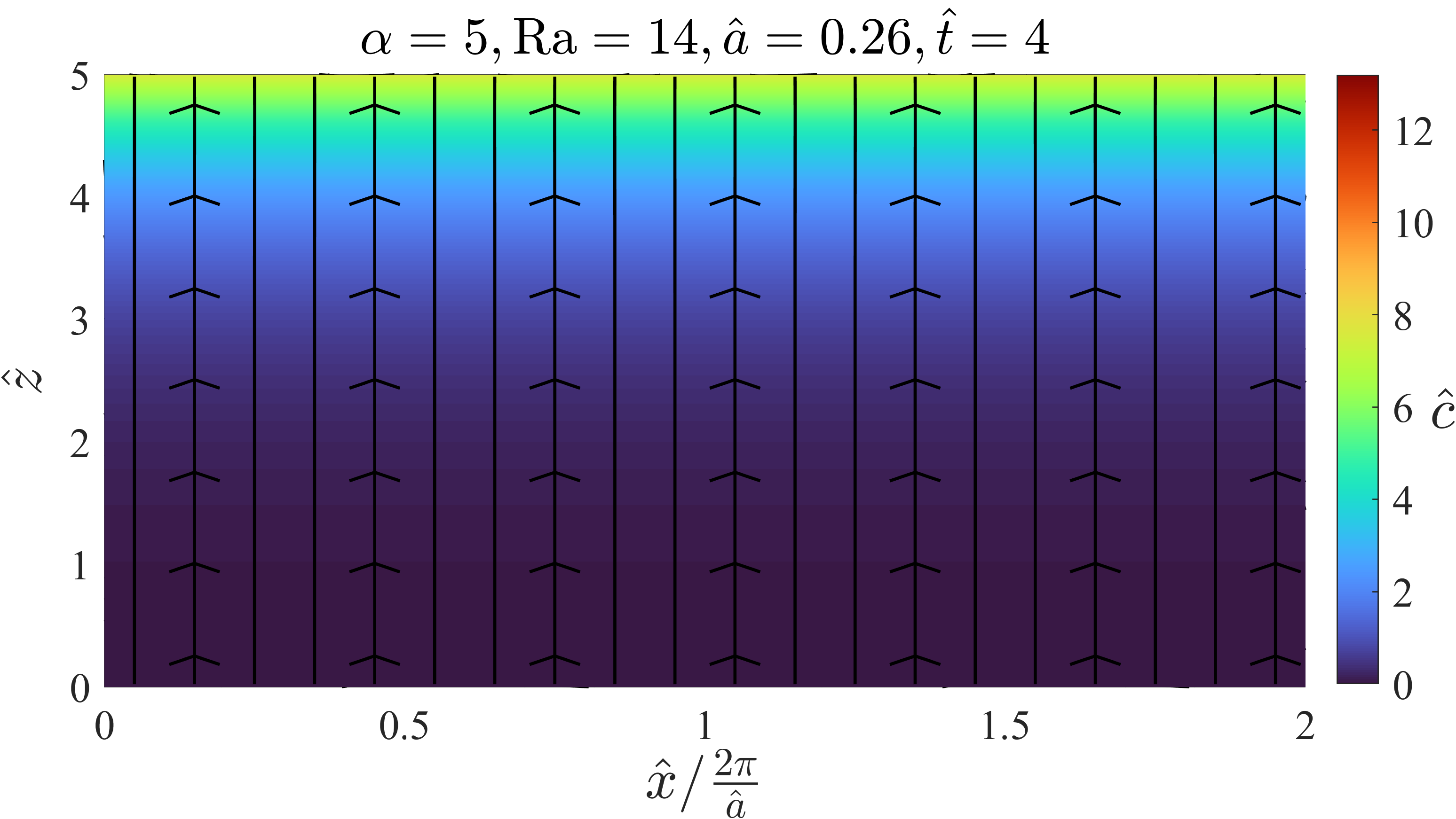
After the onset of convection, the instabilities are growing exponentially in strength until the perturbations have a sufficiently large amplitude such that nonlinear effects are not negligible anymore. The left plot in figure 10 shows the simulation result for $\alpha=5$, $\mathrm{Ra}=14$ and $\hat{a}=0.26$ at $\hat{t}=4$ (time A in figure 13), which is right before the nonlinear effects start to dominate the behaviour. At this time, we can see that the flow is still mainly characterized by a homogeneous upwards flow and the salt concentration does not visibly change in the lateral direction. Hence, the deviations from the ground state are small enough such that they are not apparent yet.

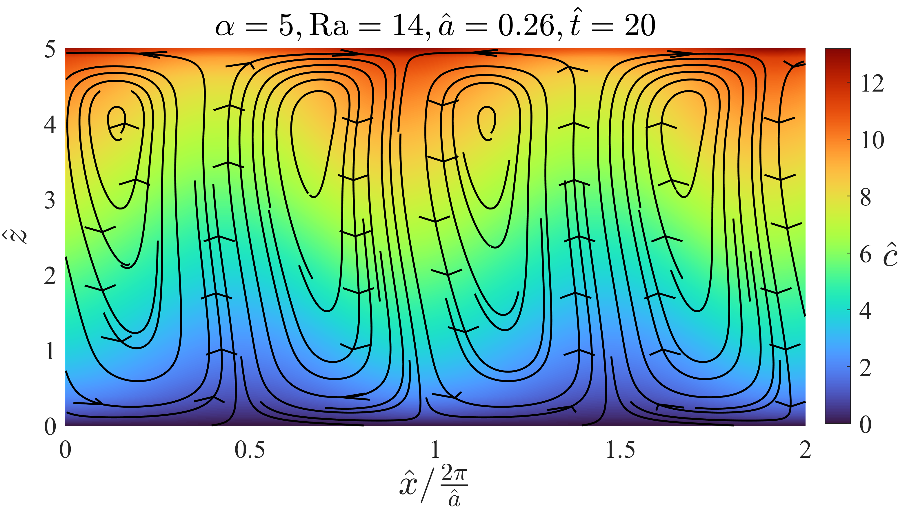
The right plot in figure 10 shows the same system slightly later at $\hat{t}=4.35$ (time B in figure 13). Here, the variations in the salt concentration at the top of the porous slab have led to the development of convection vortices. As there are alternating regions of higher and lower salt concentration at the top of the slab due to the instabilities, there are differences in buoyancy. Hence, the liquid starts to flow downwards in the areas of high salinity and continues flowing upwards in between, resulting in the convection vortices. As the vortices distribute salt from the surface to lower parts of the domain, the maximum salinity decreases for a short period, which can be seen in figure 13. At this time, however, these vortices are still confined to a small portion of the domain as the flow in the lower half of the slab still looks like the ground-state flow.

The left plot in figure 11 depicts the system at $\hat{t}=6$ (time C in figure 13), where the vortices have grown from the top and now expand to the middle of the domain. The region, in which convective flow occurs, is visibly more saline than the lower part of the porous medium. This is due to the downwards transport of salt from the top by the convection vortices. As the vortices do not span the entire domain yet, the salt transported downwards by them does not leave the porous slab and is instead partially transported upwards again. Hence, the salt concentration at the top is again increasing at this time as figure 13 shows.

The right plot in figure 11 shows the system at $\hat{t}=10$ (time D in figure 13), where the vortices begin to span the entire vertical extent of the domain. Due to the transport of salt along the regions of downwards flow, the salt fingers are starting to become more clearly visible when looking at the salt concentration profile. As the Dirichlet boundary conditions for salt and flow velocity at the bottom boundary prevent the salt fingers from growing any further here, the salt starts to accumulate at the lower part of the salt fingers. The increasing salt concentration gradient near the bottom boundary leads to more diffusive flux of salt out of the domain.

Figure 12 displays the system at $\hat{t}=20$ (time E in figure 13). As the salt concentration gradient near the bottom boundary has increased even further, enough salt diffuses out of the domain to counteract the advective salt inflow prescribed by the bottom boundary conditions. Hence, there is zero net flux of salt into the domain and the salt concentration at the top does not increase any further. This is also visible when looking at figure 13, which shows the evolution of the maximum salinity $\hat{c}_{\mathrm{max}}$ in the entire domain as measured in the simulation over time. Before $\hat{t}=4$, $\hat{c}_{\mathrm{max}}$ is almost the same as in the ground state, since the perturbations are still small in amplitude. When the perturbations become large enough, convection vortices occur and consequently the maximum salinity falls rapidly as salt is transported away from the top and more evenly distributed through the domain. However, as the vortices only span a portion of the domain, salt does not leave the domain and is instead transported to the top again. Thus, the maximum salinity is growing again after the convection vortices have built, which is also in accordance with observations by Bringedal et al. [3] for the vertically unbounded case. Only when the convection vortices have reached the bottom of the porous medium at $\hat{t}=10$, the diffusive flux of salt out of the domain is gradually increasing. Finally, in the yellow marked regime in figure 13, there is an equilibrium of diffusive outflow and advective inflow of salt at the bottom boundary, such that the maximum salinity does not grow anymore.

Even though we have only considered a specific scenario in this section, the general behavior of the development of the instabilities is similar for other dimensionless heights, Rayleigh numbers and perturbation wavenumbers. Slim [26] has decomposed the dynamics of solutal convection in a porous medium into several regimes, which can also be done in our scenario: First, perturbations are degrading until the time of onset is reached (red regime in figure 13). This corresponds to the "diffusive regime" of Slim[26]. Then, the perturbations are growing exponentially according to linear stability theory (blue regime in figure 13), which Slim calls the "linear growth regime"[26]. When instabilities, and thus the variations in the salt concentration at the surface are large enough, regions of advective downwards flow develop at the top of the porous slab and expand downwards. This regime of advective downwards flow in figure 13 corresponds to the "flux-growth regime" of Slim[26]. Now, the salt carried downwards by the vortices starts to accumulate near the bottom of the salt fingers. The large salinity gradient due to the fixed salt concentration at the bottom of the porous medium leads to a increasing diffusive flux out of the domain. Once a salt-flux equilibrium between advective inflow and diffusive outflow is reached at the bottom boundary, the maximum salinity stops growing. This is analogous to the "shut-down regime" of Slim[26] as the salt concentration profile also reaches a steady state.

References

- [1] G. B. Allison and C. J. Barnes. Estimation of evaporation from the normally “dry” lake frome in south australia. Journal of Hydrology, 78(3-4):229–242, 1985.
- [2] Werner Balser, Claudia Röscheisen, and Frank Steiner. Systems of linear ordinary differential equations–a review of three solution methods. Ulmer Seminare ber Funktionalanalysis und Differentialgleichungen, 11:53–62, 2006.
- [3] Carina Bringedal, Theresa Schollenberger, G. J. M. Pieters, C. J. van Duijn, and Rainer Helmig. Evaporation-driven density instabilities in saturated porous media. Transport in Porous Media, 143:297–341, 2022.
- [4] J Burgess. Metal Ions in Solution. Ellis Horwood series in chemical science. Ellis Horwood Ltd., Publisher New York, 1978.
- [5] Min Chan Kim and Chang Kyun Choi. Linear stability analysis on the onset of buoyancy-driven convection in liquid-saturated porous medium. Physics of Fluids, 24(4):044102, 2012.
- [6] Falin Chen and CF Chen. Onset of finger convection in a horizontal porous layer underlying a fluid layer. Journal of Heat Transfer, 1988.
- [7] Alex D. D. Craik. Wave interactions and fluid flows. Cambridge University Press, 1988.
- [8] I. N. Daliakopoulos, I. K. Tsanis, A Koutroulis, N. N. Kourgialas, A. E. Varouchakis, G. P. Karatzas, and C. J. Ritsema. The threat of soil salinity: A european scale review. Science of the total environment, 573:727–739, 2016.
- [9] Xiaolong Geng and Michel C Boufadel. Numerical modeling of water flow and salt transport in bare saline soil subjected to evaporation. Journal of Hydrology, 524:427–438, 2015.
- [10] Arkady Gilman and Jacob Bear. The influence of free convection on soil salinization in arid regions. Transport in Porous Media, 23(3):275–301, 1996.
- [11] Rainer Helmig. Multiphase flow and transport processes in the subsurface: a contribution to the modeling of hydrosystems, volume 1. Springer, 1997.
- [12] George M Homsy and Albert E Sherwood. Convective instabilities in porous media with through flow. AIChE Journal, 22(1):168–174, 1976.
- [13] Masaru Kono and Paul H Roberts. Definition of the rayleigh number for geodynamo simulation. Physics of the Earth and Planetary Interiors, 128(1-4):13–24, 2001.
- [14] John C Mason and David C Handscomb. Chebyshev polynomials. Chapman and Hall/CRC, 2002.
- [15] Emna Mejri, Rainer Helmig, and Rachida Bouhlila. Modeling of evaporation-driven multiple salt precipitation in porous media with a real field application. Geosciences, 10(10):395, 2020.
- [16] Fadl Moukalled, L Mangani, Marwan Darwish, et al. The finite volume method in computational fluid dynamics, volume 113. Springer, 2016.
- [17] J Moum and S Heiberg. An experimental determination of the diffusion constant for high in-situ salt concentrations in the norwegian marina clays. NGI, 1973.
- [18] Donald A Nield and Adrian Bejan. Internal natural convection: Heating from below. In Convection in porous media, pages 241–361. Springer, 2017.
- [19] Bülent Okur and Nesrin Örçen. Soil salinization and climate change. In Climate change and soil interactions, pages 331–350. Elsevier, 2020.
- [20] G. J. M. Pieters, C. J. van Duijn, and P. A. C. Raats. On the stability of density stratified flow below a ponded surface: comprehensive version. Technical report, Technical Report, Darcy Center, 2018.
- [21] Andrei D Polyanin. Functional separation of variables in nonlinear pdes: General approach, new solutions of diffusion-type equations. Mathematics, 8(1):90, 2020.
- [22] Salomé M. S. Shokri-Kuehni, Bernadette Raaijmakers, Theresa Kurz, Dani Or, Rainer Helmig, and Nima Shokri. Water table depth and soil salinization: From pore-scale processes to field-scale responses. Water resources research, 56(2):e2019WR026707, 2020.
- [23] Salomé M. S. Shokri-Kuehni, Mansoureh Norouzi Rad, Colin Webb, and Nima Shokri. Impact of type of salt and ambient conditions on saline water evaporation from porous media. Advances in water resources, 105:154–161, 2017.
- [24] John R Silvester. Determinants of block matrices. The Mathematical Gazette, 84(501):460–467, 2000.
- [25] Kripal Singh. Microbial and enzyme activities of saline and sodic soils. Land Degradation & Development, 27(3):706–718, 2016.
- [26] Anja C Slim. Solutal-convection regimes in a two-dimensional porous medium. Journal of fluid mechanics, 741:461–491, 2014.
- [27] Dorairaj Somasundaram. Ordinary differential equations: a first course. CRC Press, 2001.
- [28] Frances M Sutton. Onset of convection in a porous channel with net through flow. The Physics of Fluids, 13(8):1931–1934, 1970.
- [29] C. J. van Duijn, R. A. Wooding, and A. van der Ploeg. Stability criteria for the boundary layer formed by throughflow at a horizontal surface of a porous medium: extensive version. RANA Report, pages 01–05, 2001.
- [30] H Vereecken, P Burauel, J Groeneweg, E Klumpp, W Mittelstaedt, H-D Narres, T Putz, J van der Kruk, Jan Vanderborght, and F Wendland. Research at the agrosphere institute: From the process scale to the catchment scale. Vadose Zone Journal, 8(3):664–669, 2009.
- [31] R. A. Wooding, Scott W Tyler, and Ian White. Convection in groundwater below an evaporating salt lake: 1. onset of instability. Water Resources Research, 33(6):1199–1217, 1997.
- [32] R. A. Wooding, Scott W Tyler, Ian White, and P. A. Anderson. Convection in groundwater below an evaporating salt lake: 2. evolution of fingers or plumes. Water Resources Research, 33(6):1219–1228, 1997.
- [33] Anton Zettl. Sturm-liouville theory. Number 121. American Mathematical Soc., 2010.