Soft Truncation: A Universal Training Technique of
Score-based Diffusion Model for High Precision Score Estimation
Abstract
Recent advances in diffusion models bring state-of-the-art performance on image generation tasks. However, empirical results from previous research in diffusion models imply an inverse correlation between density estimation and sample generation performances. This paper investigates with sufficient empirical evidence that such inverse correlation happens because density estimation is significantly contributed by small diffusion time, whereas sample generation mainly depends on large diffusion time. However, training a score network well across the entire diffusion time is demanding because the loss scale is significantly imbalanced at each diffusion time. For successful training, therefore, we introduce Soft Truncation, a universally applicable training technique for diffusion models, that softens the fixed and static truncation hyperparameter into a random variable. In experiments, Soft Truncation achieves state-of-the-art performance on CIFAR-10, CelebA, CelebA-HQ , and STL-10 datasets.
1 Introduction
Recent advances in generative models enable the creation of highly realistic images. One direction of such modeling is likelihood-free models (Karras et al., 2019) based on minimax training. The other direction is likelihood-based models, including VAE (Vahdat & Kautz, 2020), autoregressive models (Parmar et al., 2018), and flow models (Grcić et al., 2021). Diffusion models (Ho et al., 2020) are one of the most successful likelihood-based models, where the reverse diffusion models the generative process. The success of diffusion models achieves state-of-the-art performance in image generation (Dhariwal & Nichol, 2021).
Previously, a model with the emphasis on Fréchet Inception Distance (FID), such as DDPM (Ho et al., 2020) and ADM (Dhariwal & Nichol, 2021), trains the score network with the variance weighting; whereas a model with the emphasis on Negative Log-Likelihood (NLL), such as ScoreFlow (Song et al., 2021a) and VDM (Kingma et al., 2021), trains the score network with the likelihood weighting. Such models, however, have the trade-off between NLL and FID: models with the emphasis on FID perform poorly on NLL, and vice versa. Instead of widely investigating the trade-off, they limit their work by separately training the score network on FID-favorable and NLL-favorable settings. This paper introduces Soft Truncation that significantly resolves the trade-off, with the NLL-favorable setting as the default training configuration. Soft Truncation reports a comparable FID against FID-favorable diffusion models while keeping NLL at the equivalent level of NLL-favorable models.
For that, we observe that the truncation hyperparameter is a significant hyperparameter that determines the overall scale of NLL and FID. This hyperparameter, , is the smallest diffusion time to estimate the score function, and the score function beneath is not estimated. A model with small enough favors NLL at the sacrifice on FID, and a model with relatively large is preferable to FID but has poor NLL. Therefore, we introduce Soft Truncation, which softens the fixed and static truncation hyperparameter () into a random variable () that randomly selects its smallest diffusion time at every optimization step. In every mini-batch update, we sample a new smallest diffusion time, , randomly, and the batch optimization endeavors to estimate the score function only on , rather than , by ignoring beneath . As varies by mini-batch updates, the score network successfully estimates the score function on the entire range of diffusion time on , which brings an improved FID.
There are two interesting properties of Soft Truncation. First, though Soft Truncation is nothing to do with the weighting function in its algorithmic design, surprisingly, Soft Truncation turns out to be equivalent to a diffusion model with a general weight in the expectation sense (Eq. (10)). The random variable of determines the weight function (Theorem 1), and this gives a partial reason why Soft Truncation is successful in FID as much as the FID-favorable training (Table 4), even though Soft Truncation only considers the truncation threshold in its implementation (Section 4.2). Second, once is sampled in a mini-batch optimization, Soft Truncation optimizes the log-likelihood perturbed by (Lemma 1). Thus, Soft Truncation could be framed by Maximum Perturbed Likelihood Estimation (MPLE), a generalized concept of MLE that is specifically defined only in diffusion models (Section 4.4).
2 Preliminary
Throughout this paper, we focus on continuous-time diffusion models (Song et al., 2021b). A continuous diffusion model slowly and systematically perturbs a data random variable, , into a noise variable, , as time flows. The diffusion mechanism is represented as a Stochastic Differential Equation (SDE), written by
| (1) |
where is a standard Wiener process. The drift () and the diffusion () terms are fixed, so the data variable is diffused in a fixed manner. We denote as the solution of the given SDE of Eq. (1), and we omit the subscript and superscript to denote , if no confusion is arised.
The theory of stochastic calculus indicates that there exists a corresponding reverse SDE given by
| (2) |
where the solution of this reverse SDE exactly coincides to the solution of the forward SDE of Eq. (1). Here, is the backward time differential; is a standard Wiener process flowing backward in time (Anderson, 1982); and is the probability distribution of . Henceforth, we represent as the solution of SDEs of Eqs. (1) and (2).
The diffusion model’s objective is to learn the stochastic process, , as a parametrized stochastic process, . A diffusion model builds the parametrized stochastic process as a solution of a generative SDE,
| (3) |
We construct the parametrized stochastic process by solving the generative SDE of Eq. (3) backward in time with a starting variable of , where is an noise distribution. Throughout the paper, we denote as the probability distribution of .
A diffusion model learns the generative stochastic process by minimizing the score loss (Song et al., 2021a) of
where is a weighting function that counts the contribution of each diffusion time on the loss function. This score loss is infeasible to optimize because the data score, , is intractable in general. Fortunately, is known to be equivalent to the (continuous) denoising NCSN loss (Song et al., 2021b; Song & Ermon, 2019),
up to a constant that is irrelevant to -optimization.
Two important SDEs are known to attain analytic transition probabilities, : Variance Exploding SDE (VESDE) and Variance Preserving SDE (VPSDE) (Song et al., 2021b). First, VESDE assumes and . With such specific forms of and , the transition probability of VESDE turns out to follow a Gaussian distribution of with and . Similarly, VPSDE takes and , where ; and its transition probability falls into a Gaussian distribution of with and .


Recently, Kim et al. (2022) categorize VESDE and VPSDE as a family of linear diffusions that has the SDE of
| (4) |
where and are generic -functions. Under the linear diffusions, we derive the transition probability to follow a Gaussian distribution for certain and depending on and , respectively (see Eq. (16) of Appendix A.1). We emphasize that the suggested Soft Truncation is applicable for any SDE of Eq. (1), but we limit our focus to the family of linear SDEs of Eq. (4), particularly VESDE and VPSDE among linear SDEs, to maintain the simplicity. With such a Gaussian transtion probability, the denoising NCSN loss with a linear SDE is equivalent to
if , where is a random perturbation, and is the neural network that predicts . This is the (continuous) DDPM loss (Song et al., 2021b), and the equivalence of the two losses provides a unified view of NCSN and DDPM. Hence, NCSN and DDPM are exchangeable for each other, and we take the NCSN loss as a default form of a diffusion loss throughout the paper.
The NCSN loss training is connected to the likelihood training in Song et al. (2021a) by
| (5) |
when the weighting function is the square of the diffusion term as , called the likelihood weighting.
3 Training and Evaluation of Diffusion Models in Practice
3.1 The Need of Truncation
In the family of linear SDEs, the gradient of the log transition probability satisfies , where is given to with . The denominator of converges to zero as , which leads to diverge as , as illustrated in Figure 1-(a), see Appendix A.2 for details. Therefore, the Monte-Carlo estimation of the NCSN loss is under high variance, which prevents stable training of the score network. In practice, therefore, previous research truncates the diffusion time range to , with a positive truncation hyperparameter, .
3.2 Variational Bound With Positive Truncation
For the analysis for density estimation in Section 3.3, this section derives the variational bound of the log-likelihood when a diffusion model has a positive truncation because Inequality (5) holds only with zero truncation (). Lemma 1 provides a generalization of Inequality (5), proved by applying the data processing inequality (Gerchinovitz et al., 2020) and the Girsanov theorem (Pavon & Wakolbinger, 1991; Vargas et al., 2021; Song et al., 2021a).
Lemma 1.
Lemma 1 is a generalization of Inequality (5) in that Inequality (6) collapses to Inequality (5) under the zero truncation: . If the time range is truncated to for , then from the variational inference, the log-likelihood becomes
| (7) |
where
with being the probability distribution of given and the score estimation with at . For any , we apply Lemma 1 to the right-hand-side of Inequality (7) to obtain the variational bound of the log-likelihood as
| (8) |

3.3 A Universal Phenomenon in Diffusion Training: Extremely Imbalanced Loss
To avoid the diverging issue introduced in Section 3.1, previous works in VPSDE (Song et al., 2021a; Vahdat et al., 2021) modify the loss by truncating the integration on with a fixed hyperparameter so that the score network does not estimate the score function on . Analogously, previous works in VESDE (Song et al., 2021b; Chen et al., 2022) approximate to truncate the minimum variance of the transition probability to be . Truncating diffusion time at in VPSDE is equivalent to truncating diffusion variance () in VESDE, so these two truncations on VE/VP SDEs have the identical effect on bounding the diffusion loss. Henceforth, this paper discusses the argument of truncating diffusion time (VPSDE) and diffusion variance (VESDE) exchangeably.
Figure 1 illustrates the significance of truncation in the training of diffusion models. With the truncation of strictly positive , Figure 1-(a) shows that the integrand of in the Bits-Per-Dimension (BPD) scale is still extremely imbalanced. It turns out that such extreme imbalance appears to be a universal phenomenon in training a diffusion model, and this phenomenon lasts from the beginning to the end of training.


Figure 1-(b) with the green line presents the variational bound of the log-likelihood (right-hand-side of Inequality (8)) on the -axis, and it indicates that the variational bound is sharply decreasing near the small diffusion time. Therefore, if is insufficiently small, the variational bound is not tight to the log-likelihood, and a diffusion model fails at MLE training. In addition, Figure 2 indicates that insufficiently small (or ) would also harm the microscopic sample quality. From these observations, becomes a significant hyperparameter that needs to be selected carefully.
3.4 Effect of Truncation on Model Evaluation
Figure 1-(c) reports test performances on density estimation. Figure 1-(c) illustrates that both Negative Evidence Lower Bound (NELBO) and NLL monotonically decrease by lowering because NELBO is largely contributed by small diffusion time at test time as well as training time. Therefore, it could be a common strategy to reduce as much as possible to reduce test NELBO/NLL.

| CIFAR-10 | ||
|---|---|---|
| NLL () | FID-10k () | |
| 4.95 | 6.95 | |
| 3.04 | 7.04 | |
| 2.99 | 8.17 | |
| 2.97 | 8.29 | |
On the contrary, there is a counter effect on FID for . Table 1, trained on CIFAR-10 (Krizhevsky et al., 2009) with NCSN++ (Song et al., 2021b), presents that FID is worsened as we take smaller hyperparameter for the training. It is the range of small diffusion time that significantly contributes to the variational bound in the blue line of Figure 1-(b), so the score network with a small truncation hyperparameter, or , remains unoptimized on large diffusion time. In the lens of Figure 2, therefore, the inconsistent result of Table 1 is attributed to the inaccurate score on large diffusion time.
| 6.84 | 8.04 | 8.29 |
We design an experiment to validate the above argument in Table 2. This experiment utilizes two types of score networks: 1) three alternative networks (As) with diverse trained in Table 1 experiment; 2) a network (B) with (the last row of Table 1). With these score networks, we denoise the noises by either one of the first-typed As from to a common and fixed , and we use B to further denoise from to . This further denoising step with model B enables us to compare the score accuracy on large diffusion time for models with diverse truncation hyperparameters in a fair resolution setting. Table 2 presents that the model with has the best FID, implying that the training with too small truncation would harm the sample fidelity.


Specifically, Figure 4 shows the Euclidean norm of , where each dot represents for a Monte-Carlo sample from . Here, is in the reverse drift term of the generative process, . Figure 4 illustrates that it is the large diffusion time that dominates the sampling process. Therefore, a precise score network on large diffusion time is particularly important in sample generation.
The imprecise score mainly affects the global sample context, as the denoising on small diffusion time only crafts the image in its microscopic details, illustrated in Figures 3 and 5. Figure 3 shows how the global fidelity is damaged: a man synthesized in the second row has unrealistic curly hair on his forehead, constructed on the large diffusion time. Figure 5 deepens the importance of learning a good score estimation on large diffusion time. It shows the regenerated samples by solving the generative process time reversely, starting from (Meng et al., 2021).
4 Soft Truncation: A Training Technique for a Diffusion Model
As in Section 3, the choice of is crucial for training and evaluation, but it is computationally infeasible to search for the optimal . Therefore, we introduce a training technique that predominantly mediates the need for -search by softening the fixed truncation hyperparameter into a truncation random variable so that the truncation time varies in every optimization step. Our approach successfully trains the score network on large diffusion time without sacrificing NLL. We explain the Monte-Carlo estimation of the variational bound in Section 4.1, which is the common practice of previous research but explained to emphasize how simple (though effective) Soft Truncation is, and we subsequently introduce Soft Truncation in Section 4.2.

4.1 Monte-Carlo Estimation of Truncated Variational Bound with Importance Sampling
In this section, we fix a truncation hyperparameter to be . For every batch , the Monte-Carlo estimation of the variational bound in Inequality (6) is , up to a constant irrelevant to , where with and be the corresponding Monte-Carlo samples from and , respectively. Note that this Monte-Carlo estimation is tractably computed from the analytic form of the transition probability as under linear SDEs.
Previous works (Song et al., 2021a; Huang et al., 2021) apply the importance sampling with the importance distribution of , where . It is well known (Goodfellow et al., 2016) that the Monte-Carlo variance of is minimum if the importance distribution is with , but sampling of Monte-Carlo diffusion time from at every training iteration would incur slower training speed, at least, because the importance sampling requires the score evaluation. Therefore, previous research approximates by , and becomes the approximate importance weight. This approximation, at the expense of bias, is cheap because the closed-form of the inverse Cumulative Distribution Function (CDF) is known. Unless we train the variance directly as in Kingma et al. (2021), we believe is the maximally efficient sampler as long as the training speed matters. The importance weighted Monte-Carlo estimation becomes
| (9) |
where is the Monte-Carlo sample from the importance distribution, i.e., .
The importance sampling is advantageous in both NLL and FID (Song et al., 2021a) over the uniform sampling, as the importance sampling significantly reduces the estimation variance. Figure 6-(a) illustrates the sample-by-sample loss, and the importance sampling significantly mitigates the loss scale by diffusion time compared to the scale in Figure 1-(a). However, the importance distribution satisfies as in Figure 6-(c) blue line, and most of the importance weighted Monte-Carlo time is concentrated at in Figure 7. Hence, the use of the importance sampling has a trade-off between the reduced variance (Figure 6-(a)) versus the over-sampled diffusion time near (Figure 7). Regardless of whether to use the importance sampling or not, therefore, the inaccurate score estimation on large diffusion time appears sampling-strategic-independently, and solving this pre-matured score estimation becomes a nontrivial task.
Instead of the likelihood weighting, previous works (Ho et al., 2020; Nichol & Dhariwal, 2021; Dhariwal & Nichol, 2021) train the denoising score loss with the variance weighting, . With this weighting, the importance distribution becomes the uniform distribution, , so it significantly alleviates the trade-off of using the likelihood weighting. However, the variance weighting favors FID at the sacrifice in NLL because the loss is no longer the variational bound of the log-likelihood. In contrast, the training with the likelihood weighting is leaning towards NLL than FID, so Soft Truncation is for the balanced NLL and FID, using the likelihood weighting.
4.2 Soft Truncation
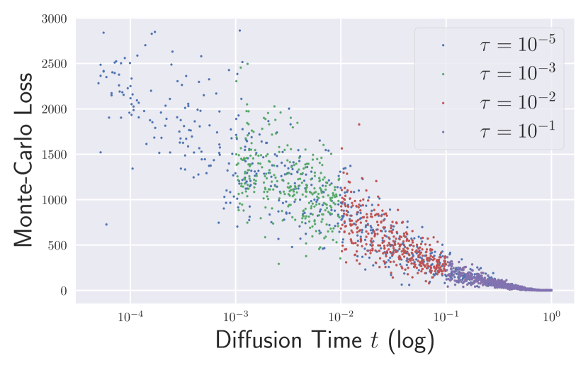
Soft Truncation releases the truncation hyperparameter from a static variable to a random variable with a probability distribution of . In every mini-batch update, Soft Truncation optimizes the diffusion model with in Eq. (9) for a sampled . In other words, for every batch , Soft Truncation optimizes the Monte-Carlo loss
with sampled from the importance distribution of , where .
Soft Truncation resolves the oversampling issue of diffusion time near , meaning that Monte-Carlo time is not concentrated on anymore. Figure 7 illustrates the quantiles of importance weighted Monte-Carlo time with Soft Truncation under and . The score network is trained more equally on diffusion time when , and as a consequence, the loss imbalance issue in each training step is also alleviated as in Figure 6-(b) with purple dots. This limited range of provides a chance to learn a score network more balanced on diffusion time. As is softened, such truncation level will vary by mini-batch updates: see the loss scales change by blue, green, red, and purple dots according to various s in Figure 6-(b). Eventually, the softened will provide a fair chance to learn the score network from small as well as large diffusion time.
4.3 Soft Truncation Equals to A Diffusion Model With A General Weight
In the original diffusion model, the loss estimation, , is just a batch-wise approximation of a population loss, . However, the target population loss of Soft Truncation, , is depending on a random variable , so the target population loss itself becomes a random variable. Therefore, we derive the expected Soft Truncation loss to reveal the connection to the original diffusion model:
up to a constant, where , by exchanging the orders of the integrations. Therefore, we conclude that Soft Truncation reduces to a diffusion model with a general weight of , see Appendix A.3:
| (10) |
4.4 Soft Truncation is Maximum Perturbed Likelihood Estimation
As explained in Section 4.3, Soft Truncation is a diffusion model with a general weight, in the expected sense. Reversely, this section analyzes a diffusion model with a general weight in view of Soft Truncation. Suppose we have a general weight . Theorem 1 implies that this general weighted diffusion loss, , is the variational bound of the perturbed KL divergence expected by . Theorem 1 collapses to Lemma 1 if for any 111If , the probability satisfies , which is a probability distribution of one mass at .. See Appendix B for the detailed statement and proof.
Theorem 1.
Suppose is a nondecreasing and nonnegative absolutely continuous function on and zero on . For the probability defined by
where ; up to a constant, the variational bound of the general weighted diffusion loss becomes
The meaning of Soft Truncation becomes clearer in view of Theorem 1. Instead of training the general weighted diffusion loss, , we optimize the truncated variational bound, . This truncated loss upper bounds the perturbed KL divergence, by Lemma 1, and Figure 1-(c) indicates that the Inequality (6) is nearly tight. Therefore, Soft Truncation could be interpreted as the Maximum Perturbed Likelihood Estimation (MPLE), where the perturbation level is a random variable. Soft Truncation is not MLE training because the Inequality 8 is not tight as demonstrated in Figure 1-(b) unless is sufficiently small.
Old wisdom is to minimize the loss variance if available for stable training. However, some optimization methods in the deep learning era (e.g., stochastic gradient descent) deliberately add noises to a loss function that eventually helps escape from a local optimum. Soft Truncation is categorized in such optimization methods that inflate the loss variance by intentionally imposing auxiliary randomness on loss estimation. This randomness is represented by the outmost expectation of , which controls the diffusion time range batch-wisely. Additionally, the loss with a sampled is the proxy of the perturbed KL divergence by , so the auxiliary randomness on loss estimation is theoretically tamed, meaning that it is not a random perturbation.
4.5 Choice of Truncation Probability Distribution
We parametrize the probability distribution of by
| (11) |
where with sufficiently small enough truncation hyperparameter. Note that it is still beneficial to remain strictly positive because a batch update with would drift the score network away from the optimal point. Figure 6-(c) illustrates the importance distribution of for varying . From the definition of Eq. (11), as , and this limiting delta distribution corresponds to the original diffusion model with the likelihood weighting. Figure 6-(c) shows that the importance distribution of with finite interpolates the likelihood weighting and the variance weighting.
With the current simple form, we experimentally find that the sweet spot is in VPSDE and in VESDE with the emphasis on the sample quality. For VPSDE, the importance distribution in Figure 6-(c) is nearly equal to that of the variance weighting if , so Soft Truncation with improves the sample fidelity, while maintaining low NLL. On the other hand, if is too small, no will be sampled near , so it hurts both sample generation and density estimation. We leave further study on searching for the optimal distribution of as future work.
![[Uncaptioned image]](https://cdn.awesomepapers.org/papers/fb468bdd-590d-494f-990d-f68cecedfd55/x12.png)
| Loss | Soft Truncation | NLL | NELBO | FID | |
|---|---|---|---|---|---|
| ODE | |||||
| CIFAR-10 | ✗ | 3.03 | 3.13 | 6.70 | |
| ✗ | 3.21 | 3.34 | 3.90 | ||
| ✗ | 3.06 | 3.18 | 6.11 | ||
| ✓ | 3.01 | 3.08 | 3.96 | ||
| ✓ | 3.03 | 3.13 | 3.45 | ||
| ImageNet32 | ✗ | 3.92 | 3.94 | 12.68 | |
| ✗ | 3.95 | 4.00 | 9.22 | ||
| ✗ | 3.93 | 3.97 | 11.89 | ||
| ✓ | 3.90 | 3.91 | 8.42 |
| SDE | Model | Loss | NLL | NELBO | FID | |
|---|---|---|---|---|---|---|
| PC | ODE | |||||
| VE | NCSN++ | 3.41 | 3.42 | 3.95 | - | |
| 3.44 | 3.44 | 2.68 | - | |||
| RVE | UNCSN++ | 2.01 | 2.01 | 3.36 | - | |
| 1.97 | 2.02 | 1.92 | - | |||
| VP | DDPM++ | 2.14 | 2.21 | 3.03 | 2.32 | |
| 2.17 | 2.29 | 2.88 | 1.90 | |||
| UDDPM++ | 2.11 | 2.20 | 3.23 | 4.72 | ||
| 2.16 | 2.28 | 2.22 | 1.94 | |||
| DDPM++ | 2.00 | 2.09 | 5.31 | 3.95 | ||
| 2.00 | 2.11 | 4.50 | 2.90 | |||
| UDDPM++ | 1.98 | 2.12 | 4.65 | 3.98 | ||
| 2.00 | 2.10 | 4.45 | 2.97 | |||
| Loss | NLL | NELBO | FID (ODE) | |
|---|---|---|---|---|
| 4.64 | 4.69 | 38.82 | ||
| 3.51 | 3.52 | 6.21 | ||
| 3.05 | 3.08 | 6.33 | ||
| 3.03 | 3.13 | 6.70 | ||
| 4.65 | 4.69 | 39.83 | ||
| 3.51 | 3.52 | 5.14 | ||
| 3.05 | 3.08 | 4.16 | ||
| 3.01 | 3.08 | 3.96 |
| Loss | NLL | NELBO | FID (ODE) |
|---|---|---|---|
| 3.24 | 3.39 | 6.27 | |
| 3.03 | 3.05 | 3.61 | |
| 3.03 | 3.13 | 3.45 | |
| 3.01 | 3.08 | 3.96 | |
| 3.02 | 3.09 | 3.98 | |
| 3.03 | 3.09 | 3.98 | |
| 3.01 | 3.10 | 6.31 | |
| 3.02 | 3.09 | 6.54 | |
| 3.01 | 3.09 | 6.70 | |
| Loss | NLL | NELBO | FID (ODE) |
|---|---|---|---|
| INDM (VP, NLL) | 2.98 | 2.98 | 6.01 |
| INDM (VP, FID) | 3.17 | 3.23 | 3.61 |
| INDM (VP, NLL) + ST | 3.01 | 3.02 | 3.88 |
Model CIFAR10 ImageNet32 CelebA CelebA-HQ STL-10 NLL () FID () IS () NLL FID IS NLL FID FID FID IS Likelihood-free Models StyleGAN2-ADA+Tuning (Karras et al., 2020) - 2.92 10.02 - - - - - - - - Styleformer (Park & Kim, 2022) - 2.82 9.94 - - - - 3.66 - 15.17 11.01 Likelihood-based Models ARDM-Upscale 4 (Hoogeboom et al., 2021) 2.64 - - - - - - - - - - VDM (Kingma et al., 2021) 2.65 7.41 - 3.72 - - - - - - - LSGM (FID) (Vahdat et al., 2021) 3.43 2.10 - - - - - - - - - NCSN++ cont. (deep, VE) (Song et al., 2021b) 3.45 2.20 9.89 - - - 2.39 3.95 7.23 - - DDPM++ cont. (deep, sub-VP) (Song et al., 2021b) 2.99 2.41 9.57 - - - - - - - - DenseFlow-74-10 (Grcić et al., 2021) 2.98 34.90 - 3.63 - - 1.99 - - - - ScoreFlow (VP, FID) (Song et al., 2021a) 3.04 3.98 - 3.84 8.34 - - - - - - Efficient-VDVAE (Hazami et al., 2022) 2.87 - - - - - 1.83 - - - - PNDM (Liu et al., 2022) - 3.26 - - - - - 2.71 - - - ScoreFlow (deep, sub-VP, NLL) (Song et al., 2021a) 2.81 5.40 - 3.76 10.18 - - - - - - Improved DDPM () (Nichol & Dhariwal, 2021) 3.37 2.90 - - - - - - - - - UNCSN++ (RVE) + ST 3.04 2.33 10.11 - - - 1.97 1.92 7.16 7.71 13.43 DDPM++ (VP, FID) + ST 2.91 2.47 9.78 - - - 2.10 1.90 - - - DDPM++ (VP, NLL) + ST 2.88 3.45 9.19 3.85 8.42 11.82 1.96 2.90 - - -
5 Experiments
This section empirically studies our suggestions on benchmark datasets, including CIFAR-10 (Krizhevsky et al., 2009), ImageNet (Van Oord et al., 2016), STL-10 (Coates et al., 2011)222We downsize the dataset from to following Jiang et al. (2021); Park & Kim (2022). CelebA (Liu et al., 2015) and CelebA-HQ (Karras et al., 2018) .
Soft Truncation is a universal training technique indepedent to model architectures and diffusion strategies. In the experiments, we test Soft Truncation on various architectures, including vanilla NCSN++, DDPM++, Unbounded NCSN++ (UNCSN++), and Unbounded DDPM++ (UDDPM++). Also, Soft Truncation is applied to various diffusion SDEs, such as VESDE, VPSDE, and Reverse VESDE (RVESDE). Although we use continuous SDEs for the diffusion strategies, Soft Truncation with the discrete model, such as DDPM (Ho et al., 2020), is a straightforward application of continuous models. Appendix D enumerates the specifications of score architectures and SDEs.
From Figure 1-(c), a sweet spot of the hard threshold is , in which NLL/NELBO are no longer improved under this threshold. As the diffusion model has no information on , we comply Kim et al. (2022) to use Inequality (7) for NLL computation and Inequality (8) for NELBO computation. Following Kim et al. (2022), we compute , rather than . It is the common practice of continuous diffusion models (Song et al., 2021b, a; Dockhorn et al., 2022) to report their performances with , but Kim et al. (2022) show that differs to by 0.05 in BPD scale when , which is quite significant. We use the uniform dequantization (Theis et al., 2016) as default, otherwise noted. For sample generation, we use either of Predictor-Corrector (PC) sampler or Ordinary Differential Equation (ODE) sampler (Song et al., 2021b). We denote as the vanilla training with -weighting, and as the training by Soft Truncation with the truncation probability of . We additionally denote for updating the network by the variance weighted loss per batch-wise update. We release our code at https://github.com/Kim-Dongjun/Soft-Truncation.
FID by Iteration Figure 8 illustrates the FID score (Heusel et al., 2017) in -axis by training steps in -axis. Figure 8 shows that Soft Truncation beats the vanilla training after 150k of training iterations.
Ablation Studies Tables 4, 4, 7, and 7 show ablation studies on various weighting functions, model architectures, SDEs, s, and probability distributions of , respectively. See Appendix E.2. Table 4 shows that Soft Truncation beats or equals to the vanilla training in all performances. We highlight that Soft Truncation with outperforms the FID-favorable model with the variance weighting with respect to FID on both CIFAR-10 and ImageNet32.
Not only comparing with the pre-existing weighting functions, such as or , Table 4 additionally reports the experimental result of a general weighting function of . From Eq. (10), Soft Truncation with and the vanilla training with coincide in their loss functions in average, i.e., . Thus, when comparing the paired experiments, Soft Truncation could be considered as an alternative way of estimating the same loss, and Table 4 implies that Soft Truncation gives better optimization than the vanilla method. This strongly implies that Soft Truncation could be a default training method for a general weighted denoising diffusion loss.
Table 4 provides two implications. First, Soft Truncation particularly boosts FID while maintaining density estimation performances under the variation of score networks and diffusion strategies. Second, Table 4 shows that Soft Truncation is effective on CelebA even when we apply Soft Truncation on the variance weighting, i.e., , but we find that this does not hold on CIFAR-10 and ImageNet32. We leave it as a future work on this extent.
Table 7 shows a contrastive trend of the vanilla training and Soft Truncation. The inverse correlation appears between NLL and FID in the vanilla training, but Soft Truncation monotonically reduces both NLL and FID by . This implies that Soft Truncation significantly reduces the effort of the search. Table 7 studies the effect of the probability distribution of in VPSDE. It shows that Soft Truncation significantly improves FID upon the experiment of on the range of . Finally, Table 7 shows that Soft Truncation also works with a nonlinear forward SDE (Kim et al., 2022), so the scope of Soft Truncation is not limited to a family of linear SDEs.
Quantitative Comparison to SOTA Table 8 compares Soft Truncation (ST) against the current best generative models. It shows that Soft Truncation achieves the state-of-the-art sample generation performances on CIFAR-10, CelebA, CelebA-HQ, and STL-10, while keeping NLL intact. In particular, we have experimented thoroughly on the CelebA dataset, and we find that Soft Truncation largely exceeds the previous best FID scores by far. In FID, Soft Truncation with DDPM++ performs 1.90, which exceeds the previous best FID of 2.92 by DDGM. Also, Soft Truncation significantly improves FID on STL-10.
6 Conclusion
This paper proposes a generally applicable training method for diffusion models. The suggested training method, Soft Truncation, is motivated from the observation that the density estimation is mostly counted on small diffusion time, while the sample generation is mostly constructed on large diffusion time. However, small diffusion time dominates the Monte-Carlo estimation of the loss function, so this imbalance contribution prevents accurate score learning on large diffusion time. Soft Truncation softens the truncation level at each mini-batch update, and this simple modification is connected to the general weighted diffusion loss and the concept of Maximum Perturbed Likelihood Estimation.
Acknowledgements
This research was supported by AI Technology Development for Commonsense Extraction, Reasoning, and Inference from Heterogeneous Data(IITP) funded by the Ministry of Science and ICT(2022-0-00077). We thank Jaeyoung Byeon and Daehan Park for their fruitful mathematical advice, and Byeonghu Na for his support of the experiments.
References
- Anderson (1982) Anderson, B. D. Reverse-time diffusion equation models. Stochastic Processes and their Applications, 12(3):313–326, 1982.
- Chen et al. (2018) Chen, R. T., Rubanova, Y., Bettencourt, J., and Duvenaud, D. K. Neural ordinary differential equations. Advances in neural information processing systems, 31, 2018.
- Chen et al. (2022) Chen, T., Liu, G.-H., and Theodorou, E. Likelihood training of schrödinger bridge using forward-backward SDEs theory. In International Conference on Learning Representations, 2022.
- Coates et al. (2011) Coates, A., Ng, A., and Lee, H. An analysis of single-layer networks in unsupervised feature learning. In Proceedings of the fourteenth international conference on artificial intelligence and statistics, pp. 215–223. JMLR Workshop and Conference Proceedings, 2011.
- Dhariwal & Nichol (2021) Dhariwal, P. and Nichol, A. Diffusion models beat gans on image synthesis. Advances in Neural Information Processing Systems, 34, 2021.
- Dockhorn et al. (2022) Dockhorn, T., Vahdat, A., and Kreis, K. Score-based generative modeling with critically-damped langevin diffusion. International Conference on Learning Representations, 2022.
- Evans (1998) Evans, L. C. Partial differential equations. Graduate studies in mathematics, 19(2), 1998.
- Gerchinovitz et al. (2020) Gerchinovitz, S., Ménard, P., and Stoltz, G. Fano’s inequality for random variables. Statistical Science, 35(2):178–201, 2020.
- Goodfellow et al. (2016) Goodfellow, I., Bengio, Y., and Courville, A. Deep learning. MIT press, 2016.
- Grcić et al. (2021) Grcić, M., Grubišić, I., and Šegvić, S. Densely connected normalizing flows. Advances in Neural Information Processing Systems, 34, 2021.
- Hazami et al. (2022) Hazami, L., Mama, R., and Thurairatnam, R. Efficient-vdvae: Less is more. arXiv preprint arXiv:2203.13751, 2022.
- Heusel et al. (2017) Heusel, M., Ramsauer, H., Unterthiner, T., Nessler, B., and Hochreiter, S. Gans trained by a two time-scale update rule converge to a local nash equilibrium. Advances in neural information processing systems, 30, 2017.
- Ho et al. (2019) Ho, J., Chen, X., Srinivas, A., Duan, Y., and Abbeel, P. Flow++: Improving flow-based generative models with variational dequantization and architecture design. In International Conference on Machine Learning, pp. 2722–2730. PMLR, 2019.
- Ho et al. (2020) Ho, J., Jain, A., and Abbeel, P. Denoising diffusion probabilistic models. Advances in Neural Information Processing Systems, 33:6840–6851, 2020.
- Hoogeboom et al. (2021) Hoogeboom, E., Gritsenko, A. A., Bastings, J., Poole, B., Berg, R. v. d., and Salimans, T. Autoregressive diffusion models. arXiv preprint arXiv:2110.02037, 2021.
- Huang et al. (2021) Huang, C.-W., Lim, J. H., and Courville, A. C. A variational perspective on diffusion-based generative models and score matching. Advances in Neural Information Processing Systems, 34, 2021.
- Jiang et al. (2021) Jiang, Y., Chang, S., and Wang, Z. Transgan: Two pure transformers can make one strong gan, and that can scale up. Advances in Neural Information Processing Systems, 34, 2021.
- Karras et al. (2018) Karras, T., Aila, T., Laine, S., and Lehtinen, J. Progressive growing of gans for improved quality, stability, and variation. In International Conference on Learning Representations, 2018.
- Karras et al. (2019) Karras, T., Laine, S., and Aila, T. A style-based generator architecture for generative adversarial networks. In Proceedings of the IEEE/CVF Conference on Computer Vision and Pattern Recognition, pp. 4401–4410, 2019.
- Karras et al. (2020) Karras, T., Aittala, M., Hellsten, J., Laine, S., Lehtinen, J., and Aila, T. Training generative adversarial networks with limited data. Advances in Neural Information Processing Systems, 33:12104–12114, 2020.
- Kim et al. (2022) Kim, D., Na, B., Kwon, S. J., Lee, D., Kang, W., and Moon, I.-C. Maximum likelihood training of implicit nonlinear diffusion models. arXiv preprint arXiv:2205.13699, 2022.
- Kingma et al. (2021) Kingma, D. P., Salimans, T., Poole, B., and Ho, J. Variational diffusion models. In Advances in Neural Information Processing Systems, 2021.
- Krizhevsky et al. (2009) Krizhevsky, A., Hinton, G., et al. Learning multiple layers of features from tiny images. 2009.
- Liu et al. (2022) Liu, L., Ren, Y., Lin, Z., and Zhao, Z. Pseudo numerical methods for diffusion models on manifolds. arXiv preprint arXiv:2202.09778, 2022.
- Liu et al. (2015) Liu, Z., Luo, P., Wang, X., and Tang, X. Deep learning face attributes in the wild. In Proceedings of the IEEE international conference on computer vision, pp. 3730–3738, 2015.
- Meng et al. (2021) Meng, C., He, Y., Song, Y., Song, J., Wu, J., Zhu, J.-Y., and Ermon, S. Sdedit: Guided image synthesis and editing with stochastic differential equations. In International Conference on Learning Representations, 2021.
- Nichol & Dhariwal (2021) Nichol, A. Q. and Dhariwal, P. Improved denoising diffusion probabilistic models. In International Conference on Machine Learning, pp. 8162–8171. PMLR, 2021.
- Oksendal (2013) Oksendal, B. Stochastic differential equations: an introduction with applications. Springer Science & Business Media, 2013.
- Park & Kim (2022) Park, J. and Kim, Y. Styleformer: Transformer based generative adversarial networks with style vector. Proceedings of the IEEE/CVF International Conference on Computer Vision, 2022.
- Parmar et al. (2022) Parmar, G., Zhang, R., and Zhu, J.-Y. On buggy resizing libraries and surprising subtleties in fid calculation. Proceedings of the IEEE/CVF International Conference on Computer Vision, 2022.
- Parmar et al. (2018) Parmar, N., Vaswani, A., Uszkoreit, J., Kaiser, L., Shazeer, N., Ku, A., and Tran, D. Image transformer. In International Conference on Machine Learning, pp. 4055–4064. PMLR, 2018.
- Pavon & Wakolbinger (1991) Pavon, M. and Wakolbinger, A. On free energy, stochastic control, and schrödinger processes. In Modeling, Estimation and Control of Systems with Uncertainty, pp. 334–348. Springer, 1991.
- Song & Ermon (2019) Song, Y. and Ermon, S. Generative modeling by estimating gradients of the data distribution. Advances in Neural Information Processing Systems, 32, 2019.
- Song & Ermon (2020) Song, Y. and Ermon, S. Improved techniques for training score-based generative models. Advances in neural information processing systems, 33:12438–12448, 2020.
- Song et al. (2021a) Song, Y., Durkan, C., Murray, I., and Ermon, S. Maximum likelihood training of score-based diffusion models. Advances in Neural Information Processing Systems, 34, 2021a.
- Song et al. (2021b) Song, Y., Sohl-Dickstein, J., Kingma, D. P., Kumar, A., Ermon, S., and Poole, B. Score-based generative modeling through stochastic differential equations. In International Conference on Learning Representations, 2021b.
- Szegedy et al. (2016) Szegedy, C., Vanhoucke, V., Ioffe, S., Shlens, J., and Wojna, Z. Rethinking the inception architecture for computer vision. In Proceedings of the IEEE conference on computer vision and pattern recognition, pp. 2818–2826, 2016.
- Theis et al. (2016) Theis, L., van den Oord, A., and Bethge, M. A note on the evaluation of generative models. In International Conference on Learning Representations (ICLR 2016), pp. 1–10, 2016.
- Vahdat & Kautz (2020) Vahdat, A. and Kautz, J. Nvae: A deep hierarchical variational autoencoder. Advances in Neural Information Processing Systems, 33:19667–19679, 2020.
- Vahdat et al. (2021) Vahdat, A., Kreis, K., and Kautz, J. Score-based generative modeling in latent space. Advances in Neural Information Processing Systems, 34, 2021.
- Van Oord et al. (2016) Van Oord, A., Kalchbrenner, N., and Kavukcuoglu, K. Pixel recurrent neural networks. In International Conference on Machine Learning, pp. 1747–1756. PMLR, 2016.
- Vargas et al. (2021) Vargas, F., Thodoroff, P., Lamacraft, A., and Lawrence, N. Solving schrödinger bridges via maximum likelihood. Entropy, 23(9):1134, 2021.
- Welling & Teh (2011) Welling, M. and Teh, Y. W. Bayesian learning via stochastic gradient langevin dynamics. In Proceedings of the 28th international conference on machine learning (ICML-11), pp. 681–688. Citeseer, 2011.
Appendix A Derivation
A.1 Transition Probability for Linear SDEs
Kim et al. (2022) has classified linear SDEs as
| (12) |
where and are real-valued functions. VESDE has and , where and are the minimum/maximum perturbation variances, respectively. It has the transition probability of
where and . VPSDE has and with the transition probability of
where and .
Analogous to VE/VP SDEs, the transition probability of the generic linear SDE of Eq. (12) is a Gaussian distribution of , where its mean and covariance functions are characterized as a system of ODEs of
| (13) | |||
| (14) |
with initial conditions to be and .
A.2 Diverging Denoising Loss
The gradient of the log transition probability, , is diverging at , where . Below Lemma 2 indicates that for any continuous score function, . This leads that the denoising score loss diverges as as illustrated in Figure 1-(a).
Lemma 2.
Let . Suppose a continuous vector field defined on a subset of a compact manifold (i.e., ) is unbounded, then there exists no such that a.e. on .
Proof of Lemma 2.
Since is an open subset of a compact manifold , for all . Also, if , is bounded. Hence, the local Lipschitzness of implies that there exists a positive such that for any and . Therefore, for any , there exists such that for all and , which leads no that satisfies a.e. on as . ∎
A.3 General Weighted Diffusion Loss
The denoising score loss is
| (17) | ||||
for any . For an appropriate class of function ,
holds by changing the order of integration. Therefore, we get
where
If , then we have
Appendix B Theorems and Proofs
Lemma 1.
For any ,
Proof.
Suppose is the path measure of the forward SDE, and is the path measure of the generative SDE. The restricted measure is defined by , where if and is a measurable set in otherwise. The restricted measure of is defined analogously. Then, by the data processing inequality, we get
| (18) |
Now, from the chain rule of KL divergences, we have
| (19) |
From the Girsanov theorem and the Martingale property, we get
| (20) |
and combining Eq. (18), (19) and (20), we have
| (21) |
Now, from
we can transform into , Eq. (21) is equivalent to
| (24) | ||||||
Now, directly applying Theorem 4 of Song et al. (2021a), the entropy of becomes
| (25) |
Therefore, from Eq. (24) and (25), we get
∎
Theorem 1.
Suppose is a weighting function of the NCSN loss. If is a nondecreasing and nonnegative absolutely continuous function on and zero on , then
Proof.
Also, plugging into Eq. (26), we have
| (28) |
Corollary 1.
Suppose is a weighting function of the NCSN loss. If is a nondecreasing and nonnegative continuous function on and zero on , then
Remark 1.
A direct extension of the proof indicates that Theorem 1 still holds when has finite jump on .
Remark 2.
The weight of is the normalizing constant of the unnormalized truncation probability, .
Appendix C Additional Score Architectures and SDEs
C.1 Additional Score Architectures: Unbounded Parametrization
From the released code of Song et al. (2021b), the NCSN++ network is modeled by , where the second argument is instead of . Experiments with or were not as good as the parametrization of , and we analyze this experimental results from Lemma 2 and Proposition 1.
Proposition 1.
Let . Suppose a continuous vector field defined on a -dimensional open subset of a compact manifold is unbounded, and the projection of on each axis is locally integrable. Then, there exists such that a.e. on .
The gradient of the log transition probability diverges at theoretically (Section A.2) and empirically (Figure 9-(a)). Here, in high-dimensional space, with is either zero or infinity. Thus, the data score is nearly identical to the gradient of the log transition probability, , and the observation of Figure 9-(a) is valid for the exact data score, as well.
Although Lemma 2 is based on , the identical result also holds for the parametrization of , so it indicates that both and cannot estimate the data score as . On the other hand, Proposition 1 implies that there exists a score function that estimates the unbounded data score asymptotically, and Proposition 1 explains the reason why the parametrization of Song et al. (2021b), i.e., , is successful on score estimation.
On top of that, we introduce another parametrization that particularly focuses on the score estimation near . We name Unbounded NCSN++ (UNCSN++) as the network of with and Unbounded DDPM++ (UDDPM++) as the network of with .
In UNCSN++, and are the hyperparameters. By acknowledging the parametrization of , we choose as . Also, to satisfy the continuously differentiability of , two hyperparameters and satisfy a system of equations with degree 2, so and are fully determined with this system of equations.


The choice of such for UDDPM++ is expected to enhance the score estimation near because the input of is distributed uniformly when we draw samples from the importance weight. Concretely, when the sampling distribution on the diffusion time is given by , the -distribution from the importance sampling becomes , which is depicted in Figure 9-(b).
Proof of Proposition 1.
Let be a standard mollifier function. If , then converges to a.e. on as (Theorem 7-(ii) of Appendix C in (Evans, 1998)). Therefore, if we define on the domain of and elsewhere, then a.e. on as .
Now, to show that is locally Lipschitz, let be a compact subset of . From , if there exists such that and for all and , then is Lipschitz on .
First, since is infinitely differentiable on its domain (Theorem 7-(i) of Appendix C in (Evans, 1998)) and , there exists such that . Second, the mollifier satisfies the uniform convergence on any compact subset of (Theorem 7-(iii) of Appendix C in (Evans, 1998)), which leads that for some . Therefore, becomes an element of . ∎
C.2 Additional SDE: Reciprocal VESDE
VESDE assumes . Then, the variance of the transition probability becomes if the diffusion starts from with the initial condition of . VESDE was originally introduced in Song & Ermon (2020) in order to satisfy the geometric property for its smooth transition of the distributional shift. Mathematically, the variance is geometric if is a constant, but VESDE losses the geometric property as illustrated in Figure 9-(c).
To attain the geometric property in VESDE, VESDE approximates the variance to be by omitting 1 from . However, this approximation leads that is not converging to in distribution because as . Indeed, a bit stronger claim is possible:
Proposition 2.
There is no SDE that has the stochastic process , defined by a transition probability , as the solution.
Proposition 2 indicates that if we approximate the variance by , then the reverse diffusion process cannot be modeled by a generative process.
Rigorously, however, if the diffusion process starts from , rather than , then the variance of the transition probability becomes , which is exactly the variance . Therefore, VESDE can be considered as a diffusion process starting from .
From this point of view, we introduce a SDE that satisfies the geometric progression property starting from . We name a new SDE as the Reciprocal VE SDE (RVESDE). RVESDE has the identical form of SDE, , with
Then, the transition probability of RVESDE becomes
As illustrated in Figure 9-(c), RVESDE attains the geometric property at the expense of having reciprocated time, . Also, RVESDE satisfies and . The existence and uniqueness of solution for RVESDE is guaranteed by Theorem 5.2.1 in (Oksendal, 2013).
Appendix D Implementation Details
D.1 Experimental Details
Training Throughout the experiments, we train our model with a learning rate of 0.0002, warmup of 5000 iterations, and gradient clipping by 1. For UNCSN++, we take , and for NCSN++, we take . On ImageNet32 training of the likelihood weighting and the variance weighting without Soft Truncation, we take , following the setting of Song et al. (2021a). Otherwise, we take . For other hyperparameters, we run our experiments according to Song et al. (2021b, a).
On datasets of resolution , we use the batch size of 128, which consumes about 48Gb GPU memory. On STL-10 with resolution , we use the batch size of 192, and on datasets of resolution , we experiment with 128 batch size. The batch size for the datasets of resolution is 40, which takes nearly 120Gb of GPU memory. On the dataset of resolution, we use the batch size of 16, which takes around 120Gb of GPU memory. We use five NVIDIA RTX-3090 GPU machines to train the model exceeding 48Gb, and we use a pair of NVIDIA RTX-3090 GPU machines to train the model that consumes less than 48Gb.
Evaluation We apply the EMA with rate of 0.999 on NCSN++/UNCSN++ and 0.9999 on DDPM++/UDDPM++. For the density estimation, we obtain the NLL performance by the Instantaneous Change of Variable (Song et al., 2021b; Chen et al., 2018). We choose to integrate the instantaneous change-of-variable of the probability flow as default, even for the ImageNet32 dataset. In spite that Song et al. (2021b, a) integrates the change-of-variable formula with the starting variable to be , Table 5 of Kim et al. (2022) analyzes that there are significant difference between starting from and , if is not small enough. Therefore, we follow Kim et al. (2022) to compute . However, to compare with the baseline models, we also evaluate the way Song et al. (2021b, a) and Vahdat et al. (2021) compute NLL. We denote the way of Kim et al. (2022) as after correction and Song et al. (2021a) as before correction, throughout the appendix. We dequantize the data variable by the uniform dequantization (Ho et al., 2019) for both after-and-before corrections. In the main paper, we only report the after correction performances.
For the sampling, we apply the Predictor-Corrector (PC) algorithm introduced in Song et al. (2021b). We set the signal-to-noise ratio as 0.16 on datasets, 0.17 on and datasets, 0.075 on 256256 sized datasets, and 0.15 on . On datasets less than resolution, we iterate 1,000 steps for the PC sampler, while we apply 2,000 steps on the other high-dimensional datasets. Throughout the experiments for VESDE, we use the reverse diffusion (Song et al., 2021b) for the predictor algorithm and the annealed Langevin dynamics (Welling & Teh, 2011) for the corrector algorithm. For VPSDE, we use the Euler-Maruyama for the predictor algorithm, and we do not use any corrector algorithm.
We compute the FID score (Song et al., 2021b) based on the modified Inception V1 network333https://tfhub.dev/tensorflow/tfgan/eval/inception/1 using the tensorflow-gan package for CIFAR-10 dataset, and we use the clean-FID (Parmar et al., 2022) based on the Inception V3 network (Szegedy et al., 2016) for the remaining datasets. We note that FID computed by (Parmar et al., 2022) reports a higher FID score compared to the original FID calculation444See https://github.com/GaParmar/clean-fid for the detailed experimental results..
Appendix E Additional Experimental Results
E.1 Ablation Study on Reconstruction Term
| Loss | Soft Truncation | Reconstruction Term for Training | NLL | NELBO | FID | ||
| (before correction) | (after correction) | (without residual) | (with residual) | ODE | |||
| ✗ | ✗ | 2.97 | 3.03 | 3.11 | 3.13 | 6.70 | |
| ✗ | ✓ | 3.01 | 2.99 | 3.07 | 3.09 | 6.93 | |
| ✓ | ✗ | 2.98 | 3.01 | 3.08 | 3.08 | 3.96 | |
| ✓ | ✓ | 2.95 | 2.98 | 3.04 | 3.04 | 4.23 | |
Table 9 presents that the training with the reconstruction term outperforms the training without the reconstruction term on NLL/NELBO with the sacrifice on sample generation. If is fixed as , then the bound
is tight enough to estimate the negative log-likelihood. However, if is a subject of random variable, then the bound is not tight to the negative log-likelihood, as evidenced in Figure 1-(b). On the other hand, if we do not count the reconstruction, then the bound becomes
up to a constant, and this bound becomes tight regardless of , which is evidenced in Figure 1-(c). This is why we call Soft Truncation as Maximum Perturbed Likelihood Estimation (MPLE).
| Dataset | Loss | Soft Truncation | NLL | NELBO | FID | ||
|---|---|---|---|---|---|---|---|
| after correction | before correction | with residual | without residual | ODE | |||
| CIFAR-10 | ✗ | 3.03 | 2.97 | 3.13 | 3.11 | 6.70 | |
| ✗ | 3.21 | 3.16 | 3.34 | 3.32 | 3.90 | ||
| ✗ | 3.06 | 3.02 | 3.18 | 3.14 | 6.11 | ||
| ✓ | 3.01 | 2.98 | 3.08 | 3.08 | 3.96 | ||
| ImageNet32 | ✗ | 3.92 | 3.90 | 3.94 | 3.95 | 12.68 | |
| ✗ | 3.95 | 3.96 | 4.00 | 4.01 | 9.22 | ||
| ✗ | 3.93 | 3.92 | 3.97 | 3.98 | 11.89 | ||
| ✓ | 3.90 | 3.87 | 3.92 | 3.92 | 9.52 | ||
| ✓ | 3.90 | 3.88 | 3.91 | 3.91 | 8.42 | ||
| SDE | Model | Loss | NLL | NELBO | FID | |||
|---|---|---|---|---|---|---|---|---|
| after correction | before correction | with residual | without residual | PC | ODE | |||
| VE | NCSN++ | 3.41 | 2.37 | 3.42 | 3.96 | 3.95 | - | |
| 3.44 | 2.42 | 3.44 | 3.97 | 2.68 | - | |||
| RVE | UNCSN++ | 2.01 | 1.96 | 2.01 | 2.17 | 3.36 | - | |
| 1.97 | 1.91 | 2.02 | 2.18 | 1.92 | - | |||
| VP | DDPM++ | 2.14 | 2.07 | 2.21 | 2.22 | 3.03 | 2.32 | |
| 2.17 | 2.08 | 2.29 | 2.26 | 2.88 | 1.90 | |||
| UDDPM++ | 2.11 | 2.07 | 2.20 | 2.21 | 3.23 | 4.72 | ||
| 2.16 | 2.08 | 2.28 | 2.25 | 2.22 | 1.94 | |||
| DDPM++ | 2.00 | 1.93 | 2.09 | 2.09 | 5.31 | 3.95 | ||
| 2.00 | 1.94 | 2.11 | 2.11 | 4.50 | 2.90 | |||
| UDDPM++ | 1.98 | 1.95 | 2.12 | 2.15 | 4.65 | 3.98 | ||
| 2.00 | 1.94 | 2.10 | 2.10 | 4.45 | 2.97 | |||
| Loss | NLL | NELBO | FID | |||
|---|---|---|---|---|---|---|
| after correction | before correction | with residual | without residual | ODE | ||
| 4.64 | 4.02 | 4.69 | 5.20 | 38.82 | ||
| 3.51 | 3.20 | 3.52 | 3.90 | 6.21 | ||
| 3.05 | 2.98 | 3.08 | 3.24 | 6.33 | ||
| 3.03 | 2.97 | 3.13 | 3.11 | 6.70 | ||
| 4.65 | 4.03 | 4.69 | 5.20 | 39.83 | ||
| 3.51 | 3.21 | 3.52 | 3.88 | 5.14 | ||
| 3.05 | 2.98 | 3.08 | 3.24 | 4.16 | ||
| 3.01 | 2.98 | 3.08 | 3.08 | 3.96 | ||
| Loss | NLL | NELBO | FID | ||
|---|---|---|---|---|---|
| after correction | before correction | with residual | without residual | ODE | |
| 3.24 | 3.16 | 3.39 | 3.34 | 6.27 | |
| 3.03 | 3.00 | 3.05 | 3.05 | 3.61 | |
| 3.03 | 2.99 | 3.13 | 3.13 | 3.45 | |
| 3.01 | 2.98 | 3.08 | 3.08 | 3.96 | |
| 3.02 | 2.99 | 3.09 | 3.10 | 3.98 | |
| 3.03 | 2.99 | 3.09 | 3.09 | 3.98 | |
| 3.01 | 2.97 | 3.10 | 3.09 | 6.31 | |
| 3.02 | 2.96 | 3.09 | 3.09 | 6.54 | |
| 3.01 | 2.95 | 3.09 | 3.07 | 6.70 | |
| Loss | NLL | NELBO | FID | ||
|---|---|---|---|---|---|
| after correction | before correction | with residual | without residual | ODE | |
| 2.97 | 2.94 | 2.97 | 2.96 | 6.06 | |
| 3.17 | 3.11 | 3.23 | 3.18 | 3.61 | |
| 3.01 | 2.98 | 3.02 | 3.01 | 3.89 | |
E.2 Full Tables
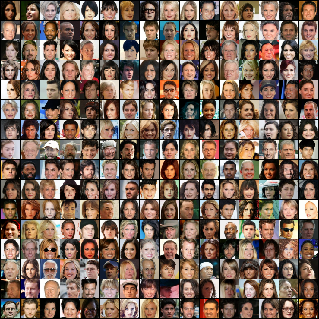
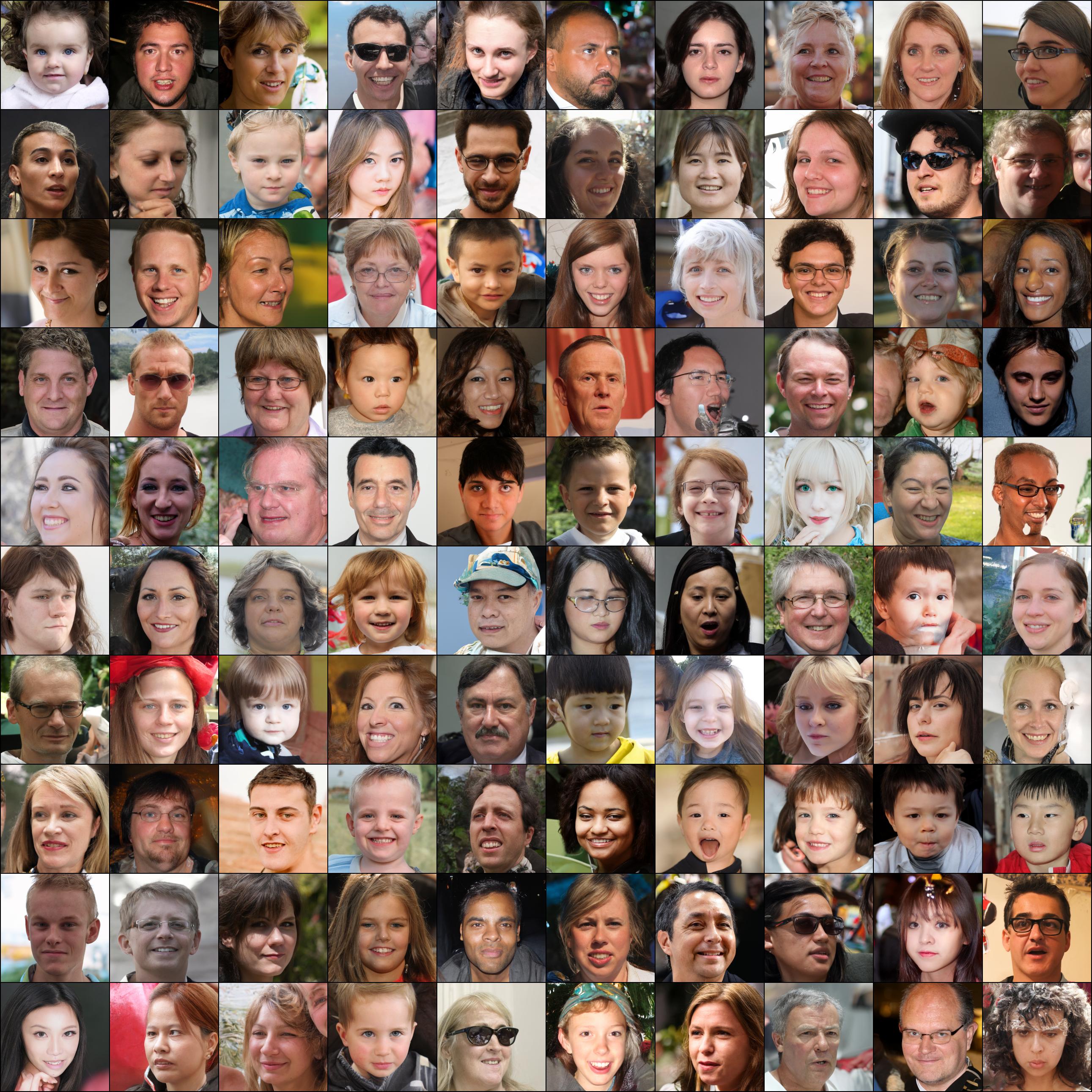
E.3 Generated Samples
Figure 10 shows how images are created from the trained model, and Figures from 11 to 16 present non-cherry picked generated samples of the trained model.