This paper was converted on www.awesomepapers.org from LaTeX by an anonymous user.
Want to know more? Visit the Converter page.

Soft-Minimum and Soft-Maximum Barrier Functions for
Safety with Actuation Constraints

Pedram Rabiee [email protected]    Jesse B. Hoagg [email protected] Department of Mechanical and Aerospace Engineering, University of Kentucky, Lexington, KY 40506
Abstract

This paper presents two new control approaches for guaranteed safety (remaining in a safe set) subject to actuator constraints (the control is in a convex polytope). The control signals are computed using real-time optimization, including linear and quadratic programs subject to affine constraints, which are shown to be feasible. The first control method relies on a soft-minimum barrier function that is constructed using a finite-time-horizon prediction of the system trajectories under a known backup control. The main result shows that the control is continuous and satisfies the actuator constraints, and a subset of the safe set is forward invariant under the control. Next, we extend this method to allow from multiple backup controls. This second approach relies on a combined soft-maximum/soft-minimum barrier function, and it has properties similar to the first. We demonstrate these controls on numerical simulations of an inverted pendulum and a nonholonomic ground robot.

keywords:
Control of constrained systems, Optimization-based controller synthesis, Nonlinear predictive control, Safety
thanks: This work is supported in part by the National Science Foundation (1849213,1932105) and the Air Force Office of Scientific Research (FA9550-20-1-0028).

,

1 Introduction

Robots and autonomous systems are often required to respect safety-critical constraints while achieving a specified task [1, 2]. Safety constraints can be achieved by determining a control that makes a designated safe set 𝒮sn{\mathcal{S}}_{\rm s}\subset{\mathbb{R}}^{n} forward invariant with respect to the closed-loop dynamics [3], that is, designing a control for which the state is guaranteed to remain in 𝒮s{\mathcal{S}}_{\rm s}. Approaches that address safety using set invariance include reachability methods [4, 5], model predictive control [6, 7, 8], and barrier function (BF) methods (e.g., [9, 10, 11, 12, 13, 14, 15]).

Barrier functions are employed in a variety of ways. For example, they are used for Lyapunov-like control design and analysis [9, 10, 11, 12]. As another example, the control barrier function (CBF) approaches in [13, 14, 15] compute the control signal using real-time optimization. These optimization-based methods can be modular in that they often combine a nominal performance controller (which may not attempt to respect safety) with a safety filter that performs a real-time optimization using CBF constraints to generate a control that guarantees safety. This real-time optimization is often formulated as an instantaneous minimum-intervention problem, that is, the problem of finding a control at the current time instant that is as close as possible to the nominal performance control while satisfying the CBF safety constraints.

Barrier-function methods typically rely on the assumption that 𝒮s{\mathcal{S}}_{\rm s} is control forward invariant (i.e., there exists a control that makes 𝒮s{\mathcal{S}}_{\rm s} forward invariant). For systems without actuator constraints (i.e., input constraints), control forward invariance is satisfied under relatively minor structural assumptions (e.g., constant relative degree). In this case, the control can be generated from a quadratic program that employs feasible CBF constraints (e.g., [13, 14, 15]). In contrast, actuator constraints can prevent 𝒮s{\mathcal{S}}_{\rm s} from being control forward invariant. In this case, it may be possible to compute a control forward invariant subset of 𝒮s{\mathcal{S}}_{\rm s} using methods such as Minkowski operations [16], sum-of-squares [17, 18], approximate solutions of a Hamilton-Jacobi partial differential equation [19], or sampling [20]. However, these methods may not scale to high-dimensional systems.

Another approach to address safety with actuator constraints is to use a prediction of the system trajectories into the future to obtain a control forward invariant subset of 𝒮s{\mathcal{S}}_{\rm s}. For example, [21] uses the trajectory under a backup control. However, [21] uses an infinite time horizon prediction, which limits applicability. In contrast, [22, 23] determine a control forward invariant subset of 𝒮s{\mathcal{S}}_{\rm s} from a BF constructed from a finite-horizon prediction under a backup control. This BF uses the minimum function, which is not continuously differentiable and cannot be used directly to form a BF constraint for real-time optimization. Thus, [22, 23] replace the original BF by a finite number of continuously differentiable BFs. However, the number of substitute BFs (and thus optimization constraints) increases as the prediction horizon increases, and these multiple BF constraints can be conservative. It is also worth noting that [22, 23] do not guarantee feasibility of the optimization with these multiple BF constraints. Related approaches are in [24, 25, 26].

This paper makes several new contributions. First, we present a soft-minimum BF that uses a finite-horizon prediction of the system trajectory under a backup control. We show that this BF describes a control forward invariant (subject to actuator constraints) subset of 𝒮s{\mathcal{S}}_{\rm s}. Since the soft-minimum BF is continuously differentiable, it can be used to form a single non-conservative BF constraint regardless of the prediction horizon. The soft-minimum BF facilitates the paper’s second contribution, namely, a real-time optimization-based control that guarantees safety with actuator constraints. Notably, the optimization required to compute the control is convex with guaranteed feasibility. Next, we extend this approach to allow from multiple backup controls by using a novel soft-maximum/soft-minimum BF. In comparison to the soft-minimum BF, the soft-maximum/soft-minimum BF (with multiple backup controls) can yield a larger control forward invariant subset of 𝒮s{\mathcal{S}}_{\rm s}. Some preliminary results on the soft-minimum BF appear in [27].

2 Notation

Let ρ>0\rho>0, and consider softminρ,softmaxρ:N\mbox{softmin}_{\rho},\mbox{softmax}_{\rho}:{\mathbb{R}}^{N}\to{\mathbb{R}} defined by

softminρ(z1,,zN)\displaystyle\mbox{softmin}_{\rho}(z_{1},\ldots,z_{N}) 1ρlogi=1Neρzi,\displaystyle\triangleq-\frac{1}{\rho}\log\sum_{i=1}^{N}e^{-\rho z_{i}},
softmaxρ(z1,,zN)\displaystyle\mbox{softmax}_{\rho}(z_{1},\ldots,z_{N}) 1ρlogi=1NeρzilogNρ,\displaystyle\triangleq\frac{1}{\rho}\log\sum_{i=1}^{N}e^{\rho z_{i}}-\frac{\log N}{\rho},

which are the soft minimum and soft minimum. The next result relates soft minimum and soft maximum to the minimum and maximum.

Proposition 1.

Let z1,,zNz_{1},\ldots,z_{N}\in{\mathbb{R}}. Then,

min{z1,,zN}logNρ\displaystyle\min\,\{z_{1},\ldots,z_{N}\}-\frac{\log N}{\rho} softminρ(z1,,zN)\displaystyle\leq\mbox{softmin}_{\rho}(z_{1},\ldots,z_{N})
min{z1,,zN},\displaystyle\leq\min\,\{z_{1},\ldots,z_{N}\},

and

max{z1,,zN}logNρ\displaystyle\max\,\{z_{1},\ldots,z_{N}\}-\frac{\log N}{\rho} softmaxρ(z1,,zN)\displaystyle\leq\mbox{softmax}_{\rho}(z_{1},\ldots,z_{N})
max{z1,,zN}.\displaystyle\leq\max\,\{z_{1},\ldots,z_{N}\}.

Proposition 1 shows that as ρ\rho\to\infty, softminρ\mbox{softmin}_{\rho} and softmaxρ\mbox{softmax}_{\rho} converge to the minimum and maximum. Thus, softminρ\mbox{softmin}_{\rho} and softmaxρ\mbox{softmax}_{\rho} are smooth approximations of the minimum and maximum. Note that if N>1N>1, then the soft minimum is strictly less than the minimum.

For a continuously differentiable function η:nl\eta\colon{\mathbb{R}}^{n}\to{\mathbb{R}}^{l}, let η:nl×n\eta^{\prime}\colon{\mathbb{R}}^{n}\to{\mathbb{R}}^{l\times n} be defined by η(x)=η(x)x\eta^{\prime}(x)=\frac{\partial\eta(x)}{\partial x}. The Lie derivatives of η\eta along the vector field of ψ:nn×p\psi\colon{\mathbb{R}}^{n}\to{\mathbb{R}}^{n\times p} is Lψη(x)η(x)ψ(x)L_{\psi}\eta(x)\triangleq\eta^{\prime}(x)\psi(x). Let int 𝒜\mbox{int }{\mathcal{A}}, bd 𝒜\mbox{bd }{\mathcal{A}}, cl 𝒜\mbox{cl }{\mathcal{A}} denote the interior, boundary, and closure of the set 𝒜n{\mathcal{A}}\subset{\mathbb{R}}^{n}. Let a,bra,b\in{\mathbb{R}}^{r}. If each element of aa is less than or equal to the corresponding element of bb, then we write aba\preceq b.

3 Problem Formulation

Consider

x˙(t)=f(x(t))+g(x(t))u(t),\dot{x}(t)=f(x(t))+g(x(t))u(t), (1)

where f:nnf:{\mathbb{R}}^{n}\to{\mathbb{R}}^{n} and g:nn×mg:{\mathbb{R}}^{n}\to{\mathbb{R}}^{n\times m} are continuously differentiable on n{\mathbb{R}}^{n}, x(t)nx(t)\in{\mathbb{R}}^{n} is the state, x(0)=x0nx(0)=x_{0}\in{\mathbb{R}}^{n} is the initial condition, and u(t)mu(t)\in{\mathbb{R}}^{m} is the control. Let Aur×mA_{u}\in{\mathbb{R}}^{r\times m} and burb_{u}\in{\mathbb{R}}^{r}, and define

𝒰{um:Auubu}m,{\mathcal{U}}\triangleq\{u\in{\mathbb{R}}^{m}:A_{u}u\preceq b_{u}\}\subset{\mathbb{R}}^{m}, (2)

which we assume is bounded and not empty. We call uu an admissible control if for all t0t\geq 0, u(t)𝒰u(t)\in{\mathcal{U}}.

Let hs:nh_{\rm s}:{\mathbb{R}}^{n}\to{\mathbb{R}} be continuously differentiable, and define the safe set

𝒮s{xn:hs(x)0}.{\mathcal{S}}_{\rm s}\triangleq\{x\in{\mathbb{R}}^{n}\colon h_{\rm s}(x)\geq 0\}. (3)

Note that 𝒮s{\mathcal{S}}_{\rm s} is not assumed to be control forward invariant with respect to (1) where uu is an admissible control. In other words, there may not exist an admissible control uu such that if x0𝒮sx_{0}\in{\mathcal{S}}_{\rm s}, then for all t0t\geq 0, x(t)𝒮sx(t)\in{\mathcal{S}}_{\rm s}.

Next, consider the nominal desired control ud:nmu_{\rm d}:{\mathbb{R}}^{n}\to{\mathbb{R}}^{m} designed to satisfy performance specifications, which can be independent of and potentially conflict with safety. Thus, 𝒮s{\mathcal{S}}_{\rm s} is not necessarily forward invariant with respect to (1) where u=udu=u_{\rm d}. We also note that udu_{\rm d} is not necessarily an admissible control.

The objective is to design a full-state feedback control u:nmu:{\mathbb{R}}^{n}\to{\mathbb{R}}^{m} such that for all initial conditions in a subset of 𝒮s{\mathcal{S}}_{\rm s}, the following hold:

  1. (O1)

    For all t0t\geq 0, x(t)𝒮sx(t)\in{\mathcal{S}}_{\rm s}.

  2. (O2)

    For all t0t\geq 0, u(x(t))𝒰u(x(t))\in{\mathcal{U}}.

  3. (O3)

    For all t0t\geq 0, u(x(t))ud(x(t))2\|u(x(t))-u_{\rm d}(x(t))\|_{2} is small.

4 Barrier Functions Using the Trajectory Under a Backup Control

Consider a continuously differentiable backup control ub:n𝒰u_{\rm b}:{\mathbb{R}}^{n}\to{\mathcal{U}}. Let hb:nh_{\rm b}:{\mathbb{R}}^{n}\to{\mathbb{R}} be continuously differentiable, and define the backup safe set

𝒮b{xn:hb(x)0}.{\mathcal{S}}_{\rm b}\triangleq\{x\in{\mathbb{R}}^{n}\colon h_{\rm b}(x)\geq 0\}. (4)

We assume 𝒮b𝒮s{\mathcal{S}}_{\rm b}\subseteq{\mathcal{S}}_{\rm s} and make the following assumption.

Assumption 1.

If u=ubu=u_{\rm b} and x0𝒮bx_{0}\in{\mathcal{S}}_{\rm b}, then for all t0t\geq 0, x(t)𝒮bx(t)\in{\mathcal{S}}_{\rm b}.

Assumption 1 states that 𝒮b{\mathcal{S}}_{\rm b} is forward invariant with respect to (1) where u=ubu=u_{\rm b}. However, 𝒮b{\mathcal{S}}_{\rm b} may be small relative to 𝒮s{\mathcal{S}}_{\rm s}.

Consider f~:nn\tilde{f}:{\mathbb{R}}^{n}\to{\mathbb{R}}^{n} defined by

f~(x)f(x)+g(x)ub(x),\tilde{f}(x)\triangleq f(x)+g(x)u_{\rm b}(x), (5)

which is the right-hand side of the closed-loop dynamics (1) with u=ubu=u_{\rm b}. Next, let ϕ:n×[0,)n\phi:{\mathbb{R}}^{n}\times[0,\infty)\to{\mathbb{R}}^{n} satisfy

ϕ(x,τ)=x+0τf~(ϕ(x,σ))dσ,\phi(x,\tau)=x+\int_{0}^{\tau}\tilde{f}(\phi(x,\sigma))\,{\rm d}\sigma, (6)

which implies that ϕ(x,τ)\phi(x,\tau) is the solution to (1) at time τ\tau with u=ubu=u_{\rm b} and initial condition xx.

Let T>0T>0 be a time horizon, and consider h:nh_{*}:{\mathbb{R}}^{n}\to{\mathbb{R}} defined by

h(x)min{hb(ϕ(x,T)),minτ[0,T]hs(ϕ(x,τ))},h_{*}(x)\triangleq\min\,\mathopen{}\mathclose{{}\left\{h_{\rm b}(\phi(x,T)),\min_{\tau\in[0,T]}h_{\rm s}(\phi(x,\tau))}\right\}, (7)

and define

𝒮{xn:h(x)0}.{\mathcal{S}}_{*}\triangleq\{x\in{\mathbb{R}}^{n}\colon h_{*}(x)\geq 0\}. (8)

For all x𝒮x\in{\mathcal{S}}_{*}, the solution (6) under ubu_{\rm b} does not leave 𝒮s{\mathcal{S}}_{\rm s} and reaches 𝒮b{\mathcal{S}}_{\rm b} by time TT. The next result relates 𝒮{\mathcal{S}}_{*} to 𝒮b{\mathcal{S}}_{\rm b} and 𝒮s{\mathcal{S}}_{\rm s}. The result is similar to [22, Proposition 6].

Proposition 2.

Assume that ubu_{\rm b} satisfies Assumption 1. Then, 𝒮b𝒮𝒮s{\mathcal{S}}_{\rm b}\subseteq{\mathcal{S}}_{*}\subseteq{\mathcal{S}}_{\rm s}.

{pf}

Let x1𝒮bx_{1}\in{\mathcal{S}}_{\rm b}. Assumption 1 implies for all t0t\geq 0, ϕ(x1,t)𝒮b𝒮s\phi(x_{1},t)\in{\mathcal{S}}_{\rm b}\subseteq{\mathcal{S}}_{\rm s}, which implies for all t0t\geq 0, hs(ϕ(x1,t))0h_{\rm s}(\phi(x_{1},t))\geq 0 and hb(ϕ(x1,t))0h_{\rm b}(\phi(x_{1},t))\geq 0. Thus, it follows from (7) and (8) that h(x1)0h_{*}(x_{1})\geq 0, which implies x1𝒮x_{1}\in{\mathcal{S}}_{*}. Therefore, 𝒮b𝒮{\mathcal{S}}_{\rm b}\subseteq{\mathcal{S}}_{*}.

Let x2𝒮x_{2}\in{\mathcal{S}}_{*}, and (7) implies hs(x2)=hs(ϕ(x2,0))h(x2)0h_{\rm s}(x_{2})=h_{\rm s}(\phi(x_{2},0))\geq h_{*}(x_{2})\geq 0. Thus, x2𝒮sx_{2}\in{\mathcal{S}}_{\rm s}, which implies 𝒮𝒮s{\mathcal{S}}_{*}\subseteq{\mathcal{S}}_{\rm s}. \Box

The next result shows that 𝒮{\mathcal{S}}_{*} is forward invariant with respect to (1) where u=ubu=u_{\rm b}. In fact, this result shows that the state converges to 𝒮b𝒮{\mathcal{S}}_{\rm b}\subseteq{\mathcal{S}}_{*} by time TT.

Proposition 3.

Consider (1), where x0𝒮x_{0}\in{\mathcal{S}}_{*}, u=ubu=u_{\rm b}, and ubu_{\rm b} satisfies Assumption 1. Then, the following hold:

  1. (a)

    For all tTt\geq T, x(t)𝒮bx(t)\in{\mathcal{S}}_{\rm b}.

  2. (b)

    For all t0t\geq 0, x(t)𝒮x(t)\in{\mathcal{S}}_{*}.

{pf}

To prove (a), since x0𝒮x_{0}\in{\mathcal{S}}_{*}, it follows from (7) and (8) that hb(ϕ(x0,T))0h_{\rm b}(\phi(x_{0},T))\geq 0, which implies x(T)=ϕ(x0,T)𝒮bx(T)=\phi(x_{0},T)\in{\mathcal{S}}_{\rm b}. Since x(T)𝒮bx(T)\in{\mathcal{S}}_{\rm b}, Assumption 1 implies for all tTt\geq T, x(t)𝒮bx(t)\in{\mathcal{S}}_{\rm b}, which confirms (a).

To prove (b), let t10t_{1}\geq 0 and consider 2 cases: t1Tt_{1}\geq T, and t1<Tt_{1}<T. First, let t1Tt_{1}\geq T, and it follows from (a) that for all tt1t\geq t_{1}, x(t)𝒮b𝒮sx(t)\in{\mathcal{S}}_{\rm b}\subseteq{\mathcal{S}}_{\rm s}. Since, in addition, for all tt1t\geq t_{1}, x(t)=ϕ(x(t1),tt1)x(t)=\phi(x(t_{1}),t-t_{1}), it follows from (7) and (8) that h(x(t1))0h_{*}(x(t_{1}))\geq 0, which implies x(t1)𝒮x(t_{1})\in{\mathcal{S}}_{*}. Next, let t1<Tt_{1}<T. Since x0𝒮x_{0}\in{\mathcal{S}}_{*}, it follows from (7) and (8) that for all t[t1,T]t\in[t_{1},T], hs(ϕ(x0,t))0h_{\rm s}(\phi(x_{0},t))\geq 0, which implies for all t[t1,T]t\in[t_{1},T], x(t)=ϕ(x0,t)𝒮sx(t)=\phi(x_{0},t)\in{\mathcal{S}}_{\rm s}. Since, in addition, for all tTt\geq T, x(t)𝒮b𝒮sx(t)\in{\mathcal{S}}_{\rm b}\subseteq{\mathcal{S}}_{\rm s}, it follows from from (7) and (8) that h(ϕ(x0,t1))0h_{*}(\phi(x_{0},t_{1}))\geq 0, which implies x(t1)𝒮x(t_{1})\in{\mathcal{S}}_{*}. \Box

Proposition 3 implies that for all x0𝒮x_{0}\in{\mathcal{S}}_{*}, the backup control ubu_{\rm b} satisfies (O1) and (O2). However, ubu_{\rm b} does not address (O3). One approach to address (O3) is to use hh_{*} as a BF in a minimum intervention quadratic program. However, hh_{*} is not continuously differentiable. Thus, it cannot be used directly to construct a BF constraint because the constraint and associated control would not be well-defined at the locations in the state space where hh_{*} is not differentiable. This issue is addressed in [22] by using multiple BFs—one for each argument of the minimum in (7). However, (7) has infinitely many arguments because the minimum is over [0,T][0,T]. Thus, [22] uses a sampling of times. Specifically, let NN be a positive integer, and define 𝒩{0,1,,N}{\mathcal{N}}\triangleq\{0,1,\ldots,N\} and TsT/NT_{\rm s}\triangleq T/N. Then, consider h¯:n\bar{h}_{*}:{\mathbb{R}}^{n}\to{\mathbb{R}} defined by

h¯(x)min{hb(ϕ(x,NTs)),mini𝒩hs(ϕ(x,iTs))},\bar{h}_{*}(x)\triangleq\min\,\mathopen{}\mathclose{{}\left\{h_{\rm b}(\phi(x,NT_{\rm s})),\min_{i\in{\mathcal{N}}}h_{\rm s}(\phi(x,iT_{\rm s}))}\right\}, (9)

and define

𝒮¯{xn:h¯(x)0}.\bar{\mathcal{S}}_{*}\triangleq\{x\in{\mathbb{R}}^{n}\colon\bar{h}_{*}(x)\geq 0\}. (10)

The next result relates 𝒮¯\bar{\mathcal{S}}_{*} to 𝒮{\mathcal{S}}_{*} and 𝒮s{\mathcal{S}}_{\rm s}.

Proposition 4.

𝒮𝒮¯𝒮s{\mathcal{S}}_{*}\subseteq\bar{\mathcal{S}}_{*}\subseteq{\mathcal{S}}_{\rm s}.

{pf}

Let x1𝒮x_{1}\in{\mathcal{S}}_{*}, and it follows from from (7)–(10) that x1𝒮¯x_{1}\in\bar{\mathcal{S}}_{*}, which implies 𝒮𝒮¯{\mathcal{S}}_{*}\subseteq\bar{\mathcal{S}}_{*}.

Let x2𝒮¯x_{2}\in\bar{\mathcal{S}}_{*}, and (9) implies hs(x2)=hs(ϕ(x2,0))h¯(x2)0h_{\rm s}(x_{2})=h_{\rm s}(\phi(x_{2},0))\geq\bar{h}_{*}(x_{2})\geq 0. Thus, x2𝒮sx_{2}\in{\mathcal{S}}_{\rm s}, which implies 𝒮¯𝒮s\bar{\mathcal{S}}_{*}\subseteq{\mathcal{S}}_{\rm s}. \Box

The next result shows that for all x0𝒮¯x_{0}\in\bar{\mathcal{S}}_{*}, the backup control ubu_{\rm b} causes the state to remain in 𝒮¯\bar{\mathcal{S}}_{*} at the sample times Ts,2Ts,,NTsT_{\rm s},2T_{\rm s},\ldots,NT_{\rm s} and converge to 𝒮b{\mathcal{S}}_{\rm b} by time TT.

Proposition 5.

Consider (1), where x0𝒮x_{0}\in{\mathcal{S}}_{*}, u=ubu=u_{\rm b}, and ubu_{\rm b} satisfies Assumption 1. Then, the following hold:

  1. (a)

    For all tTt\geq T, x(t)𝒮bx(t)\in{\mathcal{S}}_{\rm b}.

  2. (b)

    For all i𝒩i\in{\mathcal{N}}, x(iTs)𝒮¯x(iT_{\rm s})\in\bar{\mathcal{S}}_{*}.

{pf}

To prove (a), since x0𝒮¯x_{0}\in\bar{\mathcal{S}}_{*}, it follows from (9) and (10) that hb(ϕ(x0,T))0h_{\rm b}(\phi(x_{0},T))\geq 0, which implies x(T)=ϕ(x0,T)𝒮bx(T)=\phi(x_{0},T)\in{\mathcal{S}}_{\rm b}. Since x(T)𝒮bx(T)\in{\mathcal{S}}_{\rm b}, Assumption 1 implies for all tTt\geq T, x(t)𝒮bx(t)\in{\mathcal{S}}_{\rm b}, which confirms (a).

To prove (b), let i1𝒩i_{1}\in{\mathcal{N}}. Since x0𝒮¯x_{0}\in\bar{\mathcal{S}}_{*}, it follows from (9) and (10) that for all i{i1,,N}i\in\{i_{1},\ldots,N\}, hs(ϕ(x0,iTs))0h_{\rm s}(\phi(x_{0},iT_{\rm s}))\geq 0, which implies for all i{i1,,N}i\in\{i_{1},\ldots,N\}, x(iTs)=ϕ(x0,iTs)𝒮sx(iT_{\rm s})=\phi(x_{0},iT_{\rm s})\in{\mathcal{S}}_{\rm s}. Since, in addition, for all tNTst\geq NT_{\rm s}, x(t)𝒮b𝒮sx(t)\in{\mathcal{S}}_{\rm b}\subseteq{\mathcal{S}}_{\rm s}, it follows from (9) and (10) that h¯(ϕ(x0,i1Ts))0\bar{h}_{*}(\phi(x_{0},i_{1}T_{\rm s}))\geq 0, which implies x(i1Ts)𝒮¯x(i_{1}T_{\rm s})\in\bar{\mathcal{S}}_{*}. \Box

Proposition 5 does not provide any information about the state in between the sample times. Thus, Proposition 5 does not imply that 𝒮¯\bar{\mathcal{S}}_{*} is forward invariant with respect to (1) where u=ubu=u_{\rm b}. However, we can adopt an approach similar to [22] to determine a superlevel set of h¯\bar{h}_{*} such that for all initial conditions in that superlevel set, ubu_{\rm b} keeps the state in 𝒮{\mathcal{S}}_{*} for all time. To define this superlevel set, let lsl_{\rm s} be the Lipschitz constant of hsh_{\rm s} with respect to the two norm, and define lϕsupx𝒮¯f~(x)2l_{\phi}\triangleq\sup_{x\in\bar{\mathcal{S}}_{*}}\|\tilde{f}(x)\|_{2}, which is finite if 𝒮s{\mathcal{S}}_{\rm s} is bounded. Define the superlevel set

𝒮¯{xn:h¯(x)12Tslϕls}.\underaccent{\bar}{\SSS}_{*}\triangleq\mathopen{}\mathclose{{}\left\{x\in{\mathbb{R}}^{n}:\bar{h}_{*}(x)\geq\tfrac{1}{2}T_{\rm s}l_{\phi}l_{\rm s}}\right\}. (11)

The next result combines [22, Thm. 1] and Proposition 4.

Proposition 6.

𝒮¯𝒮𝒮¯𝒮s\underaccent{\bar}{\SSS}_{*}\subseteq{\mathcal{S}}_{*}\subseteq\bar{\mathcal{S}}_{*}\subseteq{\mathcal{S}}_{\rm s}.

Together, Propositions 3 and 6 imply that for all x0𝒮¯x_{0}\in\underaccent{\bar}{\SSS}_{*}, the backup control ubu_{\rm b} keeps the state in 𝒮{\mathcal{S}}_{*} for all time. However, ubu_{\rm b} does not address (O3).

Since h¯\bar{h}_{*} is not continuously differentiable, [22] addresses (O3) using a minimum intervention quadratic program with N+1N+1 BFs—one for each of the arguments in (9). However, this approach has 3 drawbacks. First, the number of BFs increases as the time horizon TT increases or the sample time TsT_{\rm s} decreases (i.e., as NN increases). Thus, the number of affine constraints and computational complexity increases as NN increases. Second, although imposing an affine constraint for each of the N+1N+1 BFs is sufficient to ensure that h¯\bar{h}_{*} remains positive, it is not necessary. These N+1N+1 affine constraints are conservative and can limit the set of feasible solutions for the control. Third, [22] does not guarantee feasibility of the optimization used to obtain the control.

The next section uses a soft-minimum BF to approximate h¯\bar{h}_{*} and presents a control synthesis approach with guaranteed feasibility and where the number of affine constraints is fixed (i.e., independent of NN).

5 Safety-Critical Control Using Soft-Minimum Barrier Function with One Backup Control

This section presents a continuous control that guarantees safety subject to the constraint that the control is admissible (i.e., in 𝒰{\mathcal{U}}). The control is computed using a minimum intervention quadratic program with a soft-minimum BF constraint. The control also relies on a linear program to provide a feasibility metric, that is, a measure of how close the quadratic program is to becoming infeasible. Then, the control continuously transitions to the backup control ubu_{\rm b} if the feasibility metric or the soft-minimum BF are less than user-defined thresholds.

Let ρ1>0\rho_{1}>0, and consider h:nh:{\mathbb{R}}^{n}\to{\mathbb{R}} defined by

h(x)\displaystyle h(x) softminρ1(hs(ϕ(x,0)),hs(ϕ(x,Ts)),,\displaystyle\triangleq\mbox{softmin}_{\rho_{1}}(h_{\rm s}(\phi(x,0)),h_{\rm s}(\phi(x,T_{\rm s})),\ldots,
hs(ϕ(x,NTs)),hb(ϕ(x,NTs))),\displaystyle\qquad h_{\rm s}(\phi(x,NT_{\rm s})),h_{\rm b}(\phi(x,NT_{\rm s}))), (12)

which is continuously differentiable. Define

𝒮{xn:h(x)0}.{\mathcal{S}}\triangleq\{x\in{\mathbb{R}}^{n}\colon h(x)\geq 0\}. (13)

Proposition 1 implies that for all xnx\in{\mathbb{R}}^{n}, h(x)<h¯(x)h(x)<\bar{h}_{*}(x). Thus, 𝒮𝒮¯{\mathcal{S}}\subset\bar{\mathcal{S}}_{*}. Proposition 1 also implies that for sufficiently large ρ1>0\rho_{1}>0, h(x)h(x) is arbitrarily close to h¯(x)\bar{h}_{*}(x). Thus, hh is a smooth approximation of h¯\bar{h}_{*}. However, if ρ1>0\rho_{1}>0 is large, then h(x)2\|h^{\prime}(x)\|_{2} is large at points where h¯\bar{h}_{*} is not differentiable. Thus, selecting ρ1\rho_{1} is a trade-off between the conservativeness of hh and the size of h(x)2\|h^{\prime}(x)\|_{2}.

Next, let α>0\alpha>0 and ϵ[0,supx𝒮h(x))\epsilon\in[0,\sup_{x\in{\mathcal{S}}}h(x)). Consider β:n\beta\colon{\mathbb{R}}^{n}\to{\mathbb{R}} defined by

β(x)Lfh(x)+α(h(x)ϵ)+maxu^𝒰Lgh(x)u^,\beta(x)\triangleq L_{f}h(x)+\alpha(h(x)-\epsilon)+\max_{\hat{u}\in{\mathcal{U}}}L_{g}h(x)\hat{u}, (14)

where β\beta exists because 𝒰{\mathcal{U}} is not empty. Define

{xn:β(x)0},{\mathcal{B}}\triangleq\{x\in{\mathbb{R}}^{n}\colon\beta(x)\geq 0\}, (15)

The next result follows immediately from (14) and (15).

Proposition 7.

For all xx\in{\mathcal{B}}, there exists u^𝒰\hat{u}\in{\mathcal{U}} such that Lfh(x)+Lgh(x)u^+α(h(x)ϵ)0L_{f}h(x)+L_{g}h(x)\hat{u}+\alpha(h(x)-\epsilon)\geq 0.

Let κh,κβ>0\kappa_{h},\kappa_{\beta}>0 and consider γ:n\gamma\colon{\mathbb{R}}^{n}\to{\mathbb{R}} defined by

γ(x)min{h(x)ϵκh,β(x)κβ},\gamma(x)\triangleq\min\mathopen{}\mathclose{{}\left\{\frac{h(x)-\epsilon}{\kappa_{h}},\frac{\beta(x)}{\kappa_{\beta}}}\right\}, (16)

and define

Γ{xn:γ(x)0}.\Gamma\triangleq\{x\in{\mathbb{R}}^{n}\colon\gamma(x)\geq 0\}. (17)

Note that Γ\Gamma\subseteq{\mathcal{B}}. For all xΓx\in\Gamma, define

u(x)argminu^𝒰u^ud(x)22\displaystyle u_{*}(x)\triangleq\underset{\hat{u}\in{\mathcal{U}}}{\mbox{argmin}}\,\|\hat{u}-u_{\rm d}(x)\|_{2}^{2} (18a)
subject to
Lfh(x)+Lgh(x)u^+α(h(x)ϵ)0.\displaystyle L_{f}h(x)+L_{g}h(x)\hat{u}+\alpha(h(x)-\epsilon)\geq 0. (18b)

Since Γ\Gamma\subseteq{\mathcal{B}}, Proposition 7 implies that for all xΓx\in\Gamma, the quadratic program (18) has a solution.

Consider a continuous function σ:[0,1]\sigma:{\mathbb{R}}\to[0,1] such that for all a(,0]a\in(-\infty,0], σ(a)=0\sigma(a)=0; for all a[1,)a\in[1,\infty), σ(a)=1\sigma(a)=1; and σ\sigma is strictly increasing on a[0,1]a\in[0,1]. The following example provides one possible choice for σ\sigma.

Example 1.

Consider σ:[0,1]\sigma:{\mathbb{R}}\to[0,1] given by

σ(a)={0,if a0,a,if 0<a<1,1,if a1.\sigma(a)=\begin{cases}0,&\mbox{if }a\leq 0,\\ a,&\mbox{if }0<a<1,\\ 1,&\mbox{if }a\geq 1.\\ \end{cases} \triangle

Finally, define the control

u(x)={[1σ(γ(x))]ub(x)+σ(γ(x))u(x),if xΓ,ub(x),else.u(x)=\begin{cases}[1-\sigma(\gamma(x))]u_{\rm b}(x)+\sigma(\gamma(x))u_{*}(x),&\mbox{if }x\in\Gamma,\\ u_{\rm b}(x),&\mbox{else}.\end{cases} (19)

Since hh is continuously differentiable, the quadratic program (18) requires only the single affine constraint (18b) as opposed to the N+1N+1 constraints used in [22]. Since (18) has only one affine constraint, we can define the feasible set {\mathcal{B}} as the zero-superlevel set of β\beta, which is the solution to the linear program (14). Since there is only one affine constraint, we can use the homotopy in (19) to continuously transition from uu_{*} to ubu_{\rm b} as xx leaves Γ\Gamma.

Remark 1.

The control (12)–(19) is designed for the case where the relative degree of (1) and (12) is one (i.e., Lgh(x)0L_{g}h(x)\neq 0). However, this control can be applied independent of the relative degree. If Lgh(x)=0L_{g}h(x)=0, then it follows from (14)–(18) that for all xΓx\in\Gamma, the solution to the quadratic program (18) is the unconstrained minimizer, which is the desired control if ud(x)𝒰u_{\rm d}(x)\in{\mathcal{U}}. In this case, (19) implies that uu is determined from a continuous blending of udu_{\rm d} and ubu_{\rm b} based on γ\gamma (i.e., feasibility of (18) and safety). We also note that the control (12)–(19) can be generalized to address the case where the relative degree exceeds one. In this case, the linear program (14) for feasibility and the quadratic program constraint (18b) are replaced by the appropriate higher-relative-degree Lie derivative expressions (see [28, 29, 30]).

The next theorem is the main result on the control (12)–(19) that uses the soft-minimum BF approach.

Theorem 1.

Consider (1) and uu given by (12)–(19), where 𝒰{\mathcal{U}} given by (2) is bounded and nonempty, and ubu_{\rm b} satisfies Assumption 1. Then, the following hold:

  1. (a)

    uu is continuous on n{\mathbb{R}}^{n}.

  2. (b)

    For all xnx\in{\mathbb{R}}^{n}, u(x)𝒰u(x)\in{\mathcal{U}}.

  3. (c)

    Let x0𝒮¯x_{0}\in\bar{\mathcal{S}}_{*}. Assume there exists t10t_{1}\geq 0 such that x(t1)bd𝒮¯x(t_{1})\in\rm{bd\,}\bar{\mathcal{S}}_{*}. Then, there exists τ(0,Ts]\tau\in(0,T_{\rm s}] such that x(t1+τ)𝒮¯𝒮sx(t_{1}+\tau)\in\bar{\mathcal{S}}_{*}\subseteq{\mathcal{S}}_{\rm s}.

  4. (d)

    Let ϵ12Tslϕls\epsilon\geq\frac{1}{2}T_{\rm s}l_{\phi}l_{\rm s} and x0𝒮x_{0}\in{\mathcal{S}}_{*}. Then, for all t0t\geq 0, x(t)𝒮𝒮sx(t)\in{\mathcal{S}}_{*}\subseteq{\mathcal{S}}_{\rm s}.

{pf}

To prove (a), we first show that uu_{*} is continuous on Γ\Gamma. Define J(x,u^)u^ud(x)22J(x,\hat{u})\triangleq\|\hat{u}-u_{\rm d}(x)\|_{2}^{2} and Ω(x){u^𝒰:Lfh(x)+Lgh(x)u^+α(h(x)ϵ)0}\Omega(x)\triangleq\{\hat{u}\in{\mathcal{U}}:L_{f}h(x)+L_{g}h(x)\hat{u}+\alpha(h(x)-\epsilon)\geq 0\}. Let aΓa\in\Gamma\subseteq{\mathcal{B}}, and Proposition 7 implies Ω(a)\Omega(a) is not empty. Since, in addition, J(a,u^)J(a,\hat{u}) is strictly convex, 𝒰{\mathcal{U}} is convex, and (18b) with x=ax=a is convex, it follows that u(a)u_{*}(a) is unique. Next, since for all xΓx\in\Gamma, u(x)𝒰u_{*}(x)\subseteq{\mathcal{U}} is bounded, it follows that u(Γ)u_{*}(\Gamma) is bounded. Thus, cl u(Γ)\mbox{cl }u_{*}(\Gamma) is compact. Next, since 𝒰{\mathcal{U}} is a convex polytope and (18b) is affine in u^\hat{u}, it follows from [31, Remark 5.5] that Ω\Omega is continuous at aa. Finally, since u(a)u_{*}(a) exists and is unique, cl u(Γ)\mbox{cl }u_{*}(\Gamma) is compact, Ω\Omega is continuous at aa, and JJ is continuous on a×Ω(a)a\times\Omega(a), it follows from [32, Corollary 8.1] that uu_{*} is continuous at aa. Thus, uu_{*} is continuous on Γ\Gamma.

Define J2(x,u^)Lfh(x)+Lgh(x)u^+α(h(x)ϵ)J_{2}(x,\hat{u})\triangleq L_{f}h(x)+L_{g}h(x)\hat{u}+\alpha(h(x)-\epsilon), and note that (14) implies β(x)=maxu^𝒰J2(x,u^)\beta(x)=\max_{\hat{u}\in{\mathcal{U}}}J_{2}(x,\hat{u}). Since J2(x,u^)J_{2}(x,\hat{u}) is continuous on Γ×𝒰\Gamma\times{\mathcal{U}} and 𝒰{\mathcal{U}} is compact, it follows from [32, Theorem 7] that β\beta is continuous on Γ\Gamma. Thus, (17) implies γ\gamma is continuous on Γ\Gamma.

For all xΓx\in\Gamma, define b(x)[1σ(γ(x))]ub(x)+σ(γ(x))u(x)b(x)\triangleq[1-\sigma(\gamma(x))]u_{\rm b}(x)+\sigma(\gamma(x))u_{*}(x). Since uu_{*}, γ\gamma, and ubu_{\rm b} are continuous on Γ\Gamma, and σ\sigma is continuous on {\mathbb{R}}, it follows that bb is continuous on Γ\Gamma. Next, let cbd Γc\in\mbox{bd }\Gamma. Since u(c)𝒰u_{*}(c)\in{\mathcal{U}} is bounded, it follows from (16) and (17) that b(c)=ub(c)b(c)=u_{{\rm b}}(c). Since bb is continuous on Γ\Gamma, ubu_{\rm b} is continuous on n{\mathbb{R}}^{n}, and for all xbd Γx\in\mbox{bd }\Gamma, b(x)=ub(x)b(x)=u_{{\rm b}}(x), it follows from (19) that uu is continuous on n{\mathbb{R}}^{n}.

To prove (b), let dnd\in{\mathbb{R}}^{n}. Since ub(d),u(d)𝒰u_{\rm b}(d),u_{*}(d)\in{\mathcal{U}}, it follows from (2) that Auub(d)buA_{u}u_{\rm b}(d)\preceq b_{u} and Auu(d)buA_{u}u_{*}(d)\preceq b_{u}. Since, in addition, σ(γ(d))[0,1]\sigma(\gamma(d))\in[0,1], it follows that

[1σ(γ(d))]Auub(d)[1σ(γ(d))]bu,\displaystyle[1-\sigma(\gamma(d))]A_{u}u_{\rm b}(d)\preceq[1-\sigma(\gamma(d))]b_{u}, (20)
σ(γ(x))Auu(d)σ(γ(d))bu.\displaystyle\sigma(\gamma(x))A_{u}u_{*}(d)\preceq\sigma(\gamma(d))b_{u}. (21)

Next, summing (20) and (21) and using (19) yields Auu(d)buA_{u}u(d)\preceq b_{u}, which implies u(d)𝒰u(d)\in{\mathcal{U}}.

To prove (c), assume for contradiction that for all τ(0,Ts]\tau\in(0,T_{\rm s}], x(t1+τ)𝒮¯x(t_{1}+\tau)\not\in\bar{\mathcal{S}}_{*}. Since, in addition, x(t1)bd𝒮¯x(t_{1})\in\rm{bd\,}\bar{\mathcal{S}}_{*}, it follows from (10) that for all τ[0,Ts]\tau\in[0,T_{\rm s}], h¯(x(t1+τ))0\bar{h}_{*}(x(t_{1}+\tau))\leq 0. Thus, Proposition 1 implies for all τ[0,Ts]\tau\in[0,T_{\rm s}], h(x(t1+τ))<h¯(x(t1+τ))0h(x(t_{1}+\tau))<\bar{h}_{*}(x(t_{1}+\tau))\leq 0, which combined with (16) and (17) implies x(t1+τ)Γx(t_{1}+\tau)\not\in\Gamma. Next, (19) implies the for all τ[0,Ts]\tau\in[0,T_{\rm s}], u(x(t1+τ))=ub(x(t1+τ))u(x(t_{1}+\tau))=u_{\rm b}(x(t_{1}+\tau)). Hence, Proposition 5 implies x(t1+Ts)𝒮¯x(t_{1}+T_{\rm s})\in\bar{\mathcal{S}}_{*}, which is a contradiction.

To prove (d), let aΓa\in\Gamma, and (16) and (17) impliy h(a)ϵ12Tslϕlsh(a)\geq\epsilon\geq\frac{1}{2}T_{\rm s}l_{\phi}l_{\rm s}. Since, in addition, Proposition 1 implies h¯(a)>h(a)\bar{h}_{*}(a)>h(a), it follows that h¯(a)>12Tslϕls\bar{h}_{*}(a)>\frac{1}{2}T_{\rm s}l_{\phi}l_{\rm s}. Thus, (11) implies aint 𝒮¯a\in\mbox{int }\underaccent{\bar}{\SSS}_{*}, which implies Γ𝒮¯𝒮\Gamma\subset\underaccent{\bar}{\SSS}_{*}\subseteq{\mathcal{S}}_{*}.

Let t30t_{3}\geq 0, and assume for contradiction that x(t3)𝒮x(t_{3})\notin{\mathcal{S}}_{*}. Since, in addition, x0𝒮x_{0}\in{\mathcal{S}}_{*} and Γ𝒮\Gamma\subset{\mathcal{S}}_{*}, it follows that there exists t2[0,t3]t_{2}\in[0,t_{3}] such that x(t2)𝒮x(t_{2})\in{\mathcal{S}}_{*} and for all τ[t2,t3]\tau\in[t_{2},t_{3}], x(τ)Γx(\tau)\not\in\Gamma. Thus, (19) implies for all τ[t2,t3]\tau\in[t_{2},t_{3}], u(x(τ))=ub(x(τ))u(x(\tau))=u_{{\rm b}}(x(\tau)). Since, in addition, x(t2)𝒮x(t_{2})\in{\mathcal{S}}_{*}, Proposition 3 implies x(t3)𝒮x(t_{3})\in{\mathcal{S}}_{*}, which is a contradiction. \Box

Parts (a) and (b) of Theorem 1 guarantee that the control is continuous and admissible. Part (d) states that if ϵ12Tslϕls\epsilon\geq\frac{1}{2}T_{\rm s}l_{\phi}l_{\rm s}, then 𝒮{\mathcal{S}}_{*} is forward invariant under the control and xx is in 𝒮s{\mathcal{S}}_{\rm s} for all time. Part (c) shows that for any choice of ϵ>0\epsilon>0, xx is in the safe set 𝒮s{\mathcal{S}}_{\rm s} at sample times 0,Ts,2Ts,3Ts,0,T_{\rm s},2T_{\rm s},3T_{\rm s},\ldots.

The control (12)–(19) relies on the Lie derivatives in (14) and (18b). To calculate LfhL_{f}h and LghL_{g}h, note that

h(x)\displaystyle h^{\prime}(x) =hb(ϕ(x,NTs))Q(x,NTs)eρ1(h(x)hb(ϕ(x,NTs)))\displaystyle=\vphantom{\sum_{i=0}^{N}}\frac{h_{\rm b}^{\prime}(\phi(x,NT_{\rm s}))Q(x,NT_{\rm s})}{e^{-\rho_{1}(h(x)-h_{\rm b}(\phi(x,NT_{\rm s})))}}
+i=0Nhs(ϕ(x,iTs))Q(x,iTs)eρ1(h(x)hs(ϕ(x,iTs))),\displaystyle\qquad+\sum_{i=0}^{N}\frac{h_{\rm s}^{\prime}(\phi(x,iT_{\rm s}))Q(x,iT_{\rm s})}{e^{-\rho_{1}(h(x)-h_{\rm s}(\phi(x,iT_{\rm s})))}}, (22)

where Q:n×[0,)n×nQ:{\mathbb{R}}^{n}\times[0,\infty)\to{\mathbb{R}}^{n\times n} is defined by Q(x,τ)ϕ(x,τ)xQ(x,\tau)\triangleq\frac{\partial\phi(x,\tau)}{\partial x}. Differentiating (6) with respect to xx yields

Q(x,τ)=I+0τf~(ϕ(x,s))Q(x,s)ds.Q(x,\tau)=I+\int_{0}^{\tau}\tilde{f}^{\prime}(\phi(x,s))Q(x,s)\,{\rm d}s. (23)

Next, differentiating (23) with respect to τ\tau yields

Q(x,τ)τ=f~(ϕ(x,τ))Q(x,τ).\frac{\partial Q(x,\tau)}{\partial\tau}=\tilde{f}^{\prime}(\phi(x,\tau))Q(x,\tau). (24)

Note that for all xnx\in{\mathbb{R}}^{n}, Q(x,τ)Q(x,\tau) is the solution to (24), where the initial condition is Q(x,0)=IQ(x,0)=I. Thus, for all xnx\in{\mathbb{R}}^{n}, Lfh(x)L_{f}h(x) and Lgh(x)L_{g}h(x) can be calculated from (5), where ϕ(x,τ)\phi(x,\tau) is the solution to (1) under ubu_{\rm b} on the interval τ[0,T]\tau\in[0,T] with ϕ(x,0)=x\phi(x,0)=x, and Q(x,τ)Q(x,\tau) is the solution to (24) on the interval τ[0,T]\tau\in[0,T] with Q(x,0)=IQ(x,0)=I. In practice, these solutions can be computed numerically at the time instants where the control algorithm (12)–(19) is executed (i.e., the time instants where the control is updated). Algorithm 1 summarizes the implementation of (12)–(19), where δt>0\delta t>0 is the time increment for a zero-order-hold on the control.

The control (12)–(19) involves the user-selected parameters ρ1,α,κh,κβ>0\rho_{1},\alpha,\kappa_{h},\kappa_{\beta}>0. Recall that large ρ1\rho_{1} improves the soft-minimum approximation of the minimum but can also result in large h(x)2\|h^{\prime}(x)\|_{2}, which can tend to cause u˙(x(t))2\|\dot{u}(x(t))\|_{2} to be large. The quadratic program (18) shows that small α\alpha results in more conservative behavior; specifically, uu deviates more from the desired control udu_{\rm d} in order to keep the state trajectory farther away from bd 𝒮\mbox{bd }{\mathcal{S}}. The homotopy (19) and definition (16) of γ\gamma show that large κh\kappa_{h} or κβ\kappa_{\beta} cause the control uu to deviate more from the optimal control uu_{*} to the backup control ubu_{\rm b} if either the feasibility metric β\beta or the barrier function hh are small.

Input: udu_{\rm d}, ubu_{\rm b}, hbh_{\rm b}, hsh_{\rm s}, NN, TsT_{\rm s}, ρ1\rho_{1}, α\alpha, ϵ\epsilon, κh\kappa_{h}, κβ\kappa_{\beta}, σ\sigma, δt\delta t
for k=0,1,2,k=0,1,2,\ldots do
       xx(kδt)x\leftarrow x(k\delta t)
       Solve (6), (24) for {ϕ(x,iTs)}i=0N\{\phi(x,iT_{\rm s})\}_{i=0}^{N}, {Q(x,iTs)}i=0N\{Q(x,iT_{\rm s})\}_{i=0}^{N}
       Compute Lfh(x)L_{f}h(x) and Lgh(x)L_{g}h(x) using (5)
       hh\leftarrow (12), β\beta\leftarrow (14), γmin{hϵκh,βκβ}\gamma\leftarrow\min\{\frac{h-\epsilon}{\kappa_{h}},\frac{\beta}{\kappa_{\beta}}\}
       if γ<0\gamma<0 then
             uub(x)u\leftarrow u_{\rm b}(x)
      else
             uu_{*}\leftarrow solution to quadratic program (18)
             u[1σ(γ)]ub(x)+σ(γ)uu\leftarrow[1-\sigma(\gamma)]u_{\rm b}(x)+\sigma(\gamma)u_{*}
            
       end if
      
end for
Algorithm 1 Control using the soft-minimum BF quadratic program
Example 2.

Consider the inverted pendulum modeled by (1), where

f(x)=[θ˙sinθ],g(x)=[01],x=[θθ˙],f(x)=\begin{bmatrix}\dot{\theta}\\ \sin\theta\end{bmatrix},\qquad g(x)=\begin{bmatrix}0\\ 1\end{bmatrix},\qquad x=\begin{bmatrix}\theta\\ \dot{\theta}\end{bmatrix},

and θ\theta is the angle from the inverted equilibrium. Let u¯=1.5\bar{u}=1.5 and 𝒰={u:u[u¯,u¯]}{\mathcal{U}}=\{u\in{\mathbb{R}}\colon u\in[-\bar{u},\bar{u}]\}. The safe set 𝒮s{\mathcal{S}}_{\rm s} is given by (3), where hs(x)=πxph_{\rm s}(x)=\pi-\|x\|_{p}, p\|\cdot\|_{p} is the pp-norm, and p=100p=100. The backup control is ub(x)=tanhKxu_{\rm b}(x)=\tanh Kx, where K=[33]K=[\,-3\quad-3\,]. The backup safe set 𝒮b{\mathcal{S}}_{{\rm b}} is given by (4), where hb(x)=0.07xT[1.250.250.250.25]x.h_{\rm b}(x)=0.07-x^{\rm T}\mathopen{}\mathclose{{}\left[\begin{smallmatrix}1.25&0.25\\ 0.25&0.25\end{smallmatrix}}\right]x. Lyapunov’s direct method can be used to confirm that Assumption 1 is satisfied. The desired control is ud=0u_{\rm d}=0, which implies that the objective is to stay in 𝒮s{\mathcal{S}}_{\rm s} using instantaneously minimum control effort. We implement the control (12)–(19) using ρ1=100\rho_{1}=100, α=1\alpha=1, κh=κβ=0.05\kappa_{h}=\kappa_{\beta}=0.05, and σ\sigma given by Example 1. We let δt=0.1\delta t=0.1 s, N=50N=50 and Ts=0.1T_{\rm s}=0.1 s, which implies that the time horizon is T=5T=5 s.

Figure 1 shows 𝒮s{\mathcal{S}}_{\rm s}, 𝒮b{\mathcal{S}}_{\rm b}, 𝒮{\mathcal{S}}, and 𝒮¯\bar{\mathcal{S}}_{*}. Note that 𝒮𝒮¯{\mathcal{S}}\subset\bar{\mathcal{S}}_{*}. Figure 1 also provides the closed-loop trajectories for 8 initial conditions, specifically, x0=[θ00]Tx_{0}=[\,\theta_{0}\quad 0\,]^{\rm T}, where θ0{±0.5,±1,±1.5,±2}\theta_{0}\in\{\pm 0.5,\pm 1,\pm 1.5,\pm 2\}. We let ϵ=0\epsilon=0 for the initial conditions with θ0{0.5,1,1.5,2}\theta_{0}\in\{0.5,1,1.5,2\}, and we let ϵ=12Tslϕls\epsilon=\frac{1}{2}T_{\rm s}l_{\phi}l_{\rm s} for θ0{0.5,1,1.5,2}\theta_{0}\in\{-0.5,-1,-1.5,-2\}, which are the reflection of the first 4 across the origin. For the cases with ϵ=12Tslϕls\epsilon=\frac{1}{2}T_{\rm s}l_{\phi}l_{\rm s}, Theorem 1 implies that 𝒮{\mathcal{S}}_{*} is forward invariant under the control (19). The trajectories with ϵ=12Tslϕls\epsilon=\frac{1}{2}T_{\rm s}l_{\phi}l_{\rm s} are more conservative than those with ϵ=0\epsilon=0.

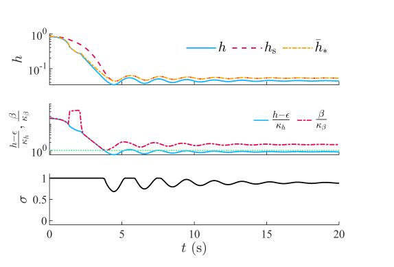
Figure 2 and 3 provide time histories for the case where x0=[ 0.50]Tx_{0}=[\,0.5\quad 0\,]^{\rm T} and ϵ=0\epsilon=0. Figure 2 shows θ\theta, θ˙\dot{\theta}, uu, udu_{\rm d}, ubu_{\rm b}, and uu_{*}. The first row of Figure 3 shows that hh, hsh_{\rm s}, and h¯\bar{h}_{*} are nonnegative for all time. The second row of Figure 3 shows hϵκh\frac{h-\epsilon}{\kappa_{h}} and βκβ\frac{\beta}{\kappa_{\beta}}. Note that β\beta is positive for all time, which implies that (18) is feasible at all points along the closed-loop trajectory. Since γ\gamma is positive for all time but is less than 11 in steady state, it follows from (19) that uu in steady state is a blend of ubu_{\rm b} and uu_{*}. \triangle

Refer to caption
Figure 1: 𝒮s{\mathcal{S}}_{\rm s}, 𝒮b{\mathcal{S}}_{\rm b}, 𝒮{\mathcal{S}}, 𝒮¯\bar{\mathcal{S}}_{*}, and closed-loop trajectories for 8 initial conditions.
Refer to caption
Figure 2: θ\theta, θ˙\dot{\theta}, uu, udu_{\rm d}, ubu_{\rm b}, and uu_{*} for x0=[0.5  0]Tx_{0}=[0.5\,\,0]^{\rm T}.
Refer to caption
Figure 3: hh, hsh_{\rm s}, h¯\bar{h}_{*}, hϵκh\frac{h-\epsilon}{\kappa_{h}}, βκβ\frac{\beta}{\kappa_{\beta}}, and σ\sigma for x0=[0.5  0]Tx_{0}=[0.5\,\,0]^{\rm T}.
Example 3.

Consider the nonholonomic ground robot modeled by (1), where

f(x)=[vcosθvsinθ00],g(x)=[00001001],x=[qxqyvθ],u=[u1u2],f(x)=\begin{bmatrix}v\cos{\theta}\\ v\sin{\theta}\\ 0\\ 0\end{bmatrix},\,g(x)=\begin{bmatrix}0&0\\ 0&0\\ 1&0\\ 0&1\end{bmatrix},\,x=\begin{bmatrix}q_{\rm x}\\ q_{\rm y}\\ v\\ \theta\end{bmatrix},\,u=\begin{bmatrix}u_{1}\\ u_{2}\end{bmatrix},

and [qxqy]T[\,q_{\rm x}\quad q_{\rm y}\,]^{\rm T} is the robot’s position in an orthogonal coordinate system, vv is the speed, and θ\theta is direction of the velocity vector (i.e., the angle from [ 10]T[\,1\quad 0\,]^{\rm T} to [q˙xq˙y]T[\,\dot{q}_{\rm x}\quad\dot{q}_{\rm y}\,]^{\rm T}). Let u¯1=4\bar{u}_{1}=4, u¯2=1\bar{u}_{2}=1, and

𝒰={[u1u2]T2:u1[u¯1,u¯1],u2[u¯2,u¯2]}.{\mathcal{U}}=\{[u_{1}\,u_{2}]^{\rm T}\in{\mathbb{R}}^{2}:u_{1}\in[-\bar{u}_{1},\bar{u}_{1}],u_{2}\in[-\bar{u}_{2},\bar{u}_{2}]\}.

Define rxqx+dcosθr_{\rm x}\triangleq q_{\rm x}+d\cos{\theta}, and ryqy+dsinθr_{\rm y}\triangleq q_{\rm y}+d\sin{\theta}, where d=1d=1, and note that [rxry]T[\,r_{\rm x}\quad r_{\rm y}\,]^{\rm T} is the position of a point-of-interest on the robot. Consider the map shown in Figure 4, which has 6 obstacles and a wall. For i{1,,6}i\in\{1,\ldots,6\}, the area outside the iith obstacle is modeled as the zero-superlevel set of

qi(x)=[ax,i(rxbx,i)ay,i(ryby,i)av,i(vbv,i)]pci,q_{i}(x)=\mathopen{}\mathclose{{}\left\|\mathopen{}\mathclose{{}\left[\begin{smallmatrix}a_{{\rm x},i}(r_{\rm x}-b_{{\rm x},i})\\ a_{{\rm y},i}(r_{\rm y}-b_{{\rm y},i})\\ a_{v,i}(v-b_{v,i})\end{smallmatrix}}\right]}\right\|_{p}-c_{i},

where bx,i,by,i,bv,i,ax,i,ay,i,av,i,ci,p>0b_{{\rm x},i},b_{{\rm y},i},b_{v,i},a_{{\rm x},i},a_{{\rm y},i},a_{v,i},c_{i},p>0 specify the location and dimensions of the iith obstacle. The area inside the wall is modeled as the zero-superlevel set of

qw(x)=c[axrxayryavv]p,q_{\rm w}(x)=c-\mathopen{}\mathclose{{}\left\|\mathopen{}\mathclose{{}\left[\begin{smallmatrix}a_{{\rm x}}r_{\rm x}\\ a_{{\rm y}}r_{\rm y}\\ a_{v}v\end{smallmatrix}}\right]}\right\|_{p},

where ax,ay,av,c,p>0a_{{\rm x}},a_{{\rm y}},a_{v},c,p>0 specify the dimension of the space inside the wall. The safe set 𝒮s{\mathcal{S}}_{\rm s} is given by (3), where hs(x)=softmin20(qw(x),q1(x),,q6(x))h_{\rm s}(x)=\mbox{softmin}_{20}(q_{\rm w}(x),q_{1}(x),\ldots,q_{6}(x)). The safe set 𝒮s{\mathcal{S}}_{\rm s} projected into the rxr_{\rm x}ryr_{\rm y} plane is shown in Figure 4. Note that 𝒮s{\mathcal{S}}_{\rm s} is also bounded in speed vv, specifically, for all x𝒮sx\in{\mathcal{S}}_{\rm s}, v[1,9]v\in[-1,9].

The backup control is ub(x)=[u¯1tanhμv0]Tu_{{\rm b}}(x)=[\,\bar{u}_{1}\tanh\mu v\quad 0\,]^{\rm T}, where μ=15\mu=-15. The backup safe set 𝒮b{\mathcal{S}}_{{\rm b}} is given by (4), where hb(x)=hs(x)100v2u¯1h_{{\rm b}}(x)=h_{\rm s}(x)-100\frac{v^{2}}{\bar{u}_{1}}. Lyapunov’s direct method can be used to confirm that Assumption 1 is satisfied. Figure 4 shows the projection of 𝒮b{\mathcal{S}}_{{\rm b}} into the rxr_{\rm x}ryr_{\rm y} plane.

Let rd2r_{{\rm d}}\in{\mathbb{R}}^{2} be the goal location, that is, the desired location for [rxry]T[\,r_{\rm x}\quad r_{\rm y}\,]^{\rm T}. Next, the desired control is ud(x)=[u¯1tanhvd(x)u¯2tanhωd(x)]Tu_{{\rm d}}(x)=[\,\bar{u}_{1}\tanh v_{{\rm d}}(x)\quad\bar{u}_{2}\tanh\omega_{{\rm d}}(x)\,]^{\rm T}, where

vd(x)\displaystyle v_{{\rm d}}(x) (μ1+μ2)v(1+μ1μ2)e1(x)+μ12de2(x)2,\displaystyle\triangleq-(\mu_{1}+\mu_{2})v-(1+\mu_{1}\mu_{2})e_{1}(x)+\frac{\mu_{1}^{2}}{d}e_{2}(x)^{2},
ωd(x)\displaystyle\omega_{{\rm d}}(x) μ1de2(x),\displaystyle\triangleq-\frac{\mu_{1}}{d}e_{2}(x),
[e1(x)e2(x)]\displaystyle\begin{bmatrix}e_{1}(x)\\ e_{2}(x)\end{bmatrix} [cosθsinθsinθcosθ]([rxry]rd),\displaystyle\triangleq\begin{bmatrix}\cos{\theta}&\sin{\theta}\\ -\sin{\theta}&\cos{\theta}\end{bmatrix}\mathopen{}\mathclose{{}\left(\begin{bmatrix}r_{\rm x}\\ r_{\rm y}\end{bmatrix}-r_{\rm d}}\right),

where μ1=μ2=0.8\mu_{1}=\mu_{2}=0.8. Note that the desired control is designed using a process similar to [33, pp. 30–31].

We implement the control (12)–(19) using ρ1=50\rho_{1}=50, α=1\alpha=1, ϵ=0\epsilon=0, κh=0.012\kappa_{h}=0.012, κβ=0.05\kappa_{\beta}=0.05, and σ\sigma given by Example 1. We let δt=0.02s\delta t=0.02\,{\rm s}, N=50N=50 and Ts=0.02sT_{\rm s}=0.02\,{\rm s}.

Figure 4 shows the closed-loop trajectories for x0=[38.500]Tx_{0}=[\,-3\quad-8.5\quad 0\quad 0\,]^{\rm T} with 3 different goal locations rd=[ 24.5]Tr_{{\rm d}}=[\,2\quad 4.5\,]^{\rm T}, rd=[10]Tr_{{\rm d}}=[\,-1\quad 0\,]^{\rm T}, and rd=[4.58]Tr_{{\rm d}}=[\,-4.5\quad 8\,]^{\rm T}. In all cases, the robot position converges to the goal location while satisfying safety and the actuator constraints.

Figures 5 and 6 show the trajectories of the relevant signals for the case where rd=[ 24.5]Tr_{{\rm d}}=[\,2\quad 4.5\,]^{\rm T}. Figure 6 shows that β\beta is positive for all time, which implies that (18) is feasible at all points along the closed-loop trajectory. Since γ\gamma is positive for all time and is greater than 11 for t>3.4st>3.4~{}{\rm s}, it follows from (19) that uu in steady state is equal to uu_{*} (as shown in Figure 2). \triangle

Refer to caption
Figure 4: 𝒮s{\mathcal{S}}_{\rm s}, 𝒮b{\mathcal{S}}_{\rm b}, and 3 closed-loop trajectories.
Refer to caption
Figure 5: qxq_{\rm x}, qyq_{\rm y}, vv, θ\theta, uu, udu_{\rm d}, ubu_{\rm b}, and uu_{*} for rd=[ 24.5]Tr_{{\rm d}}=[\,2\quad 4.5\,]^{\rm T}.
Refer to caption
Figure 6: hh, hsh_{\rm s}, h¯\bar{h}_{*}, hϵκh\frac{h-\epsilon}{\kappa_{h}}, βκβ\frac{\beta}{\kappa_{\beta}}, and σ\sigma for rd=[ 24.5]Tr_{{\rm d}}=[\,2\quad 4.5\,]^{\rm T}.

6 Soft-Maximum/Soft-Minimum Barrier Function with Multiple Backup Controls

This section extends the method from the previous section to allow for multiple backup controls by adopting a soft-maximum/soft-minimum BF. The following example illustrates the limitations of a single backup control and motivates the potential benefit of considering multiple backup controls.

Example 4.

We revisit the inverted pendulum from Example 2, where the safe set 𝒮s{\mathcal{S}}_{\rm s} is given by (3), where hs(x)=1[1π001]x100h_{\rm s}(x)=1-\mathopen{}\mathclose{{}\left\|\mathopen{}\mathclose{{}\left[\begin{smallmatrix}\frac{1}{\pi}&0\\ 0&1\end{smallmatrix}}\right]x}\right\|_{100}. We let ϵ=0\epsilon=0, N=150N=150 and Ts=0.1T_{\rm s}=0.1. Everything else is the same as in Example 2.

Figure 7 shows 𝒮s{\mathcal{S}}_{\rm s}, 𝒮b{\mathcal{S}}_{\rm b} and 𝒮{\mathcal{S}}. We note that increasing TT does not change 𝒮{\mathcal{S}}. In other words, TT was selected to yield the largest possible 𝒮{\mathcal{S}} under the backup control and safe set considered. Thus, with only one backup control, 𝒮{\mathcal{S}} cannot always be expanded by increasing TT.

Figure 7 also shows the closed-loop trajectory under Algorithm 1 with x0=[2.70]Tx_{0}=[\,-2.7\quad 0\,]^{\rm T}. The state leaves the safe set 𝒮s{\mathcal{S}}_{\rm s}. In this example, u=ubu=u_{\rm b} because that state is never in 𝒮{\mathcal{S}}. \triangle

Refer to caption
Figure 7: 𝒮s{\mathcal{S}}_{\rm s}, 𝒮b{\mathcal{S}}_{\rm b}, 𝒮{\mathcal{S}}, 𝒮¯\bar{\mathcal{S}}_{*}, and the closed-loop trajectory under Algorithm 1 with x0=[2.7  0]Tx_{0}=[\,-2.7\,\,0\,]^{\rm T}.

This section presents a method to expand 𝒮{\mathcal{S}} by using multiple backup controls. Let ν\nu be a positive integer, and consider the continuously differentiable backup controls ub1,,ubν:n𝒰u_{{\rm b}_{1}},\ldots,u_{{\rm b}_{\nu}}:{\mathbb{R}}^{n}\to{\mathcal{U}}. Let hbj:nh_{{\rm b}_{j}}:{\mathbb{R}}^{n}\to{\mathbb{R}} be continuously differentiable, and define the backup safe set

𝒮bj{xn:hbj(x)0}.{\mathcal{S}}_{{\rm b}_{j}}\triangleq\{x\in{\mathbb{R}}^{n}\colon h_{{\rm b}_{j}}(x)\geq 0\}. (25)

We assume 𝒮bj𝒮s{\mathcal{S}}_{{\rm b}_{j}}\subseteq{\mathcal{S}}_{\rm s} and make the following assumption.

Assumption 2.

For all j{1,,ν}j\in\{1,\ldots,\nu\}, if u=ubju=u_{{\rm b}_{j}} and x0𝒮bjx_{0}\in{\mathcal{S}}_{{\rm b}_{j}}, then for all t0t\geq 0, x(t)𝒮bjx(t)\in{\mathcal{S}}_{{\rm b}_{j}}.

Assumption 2 states that 𝒮bj{\mathcal{S}}_{{\rm b}_{j}} is forward invariant with respect to (1) where u=ubju=u_{{\rm b}_{j}}. This is equivalent to Assumption 1 for each backup control.

Let f~j:nn\tilde{f}_{j}:{\mathbb{R}}^{n}\to{\mathbb{R}}^{n} be defined by (5), where f~\tilde{f} and ubu_{\rm b} are replaced by f~j\tilde{f}_{j} and ubju_{{\rm b}_{j}}. Similarly, let ϕj:n×[0,)n\phi_{j}:{\mathbb{R}}^{n}\times[0,\infty)\to{\mathbb{R}}^{n} be defined by (6), where ϕ\phi and f~\tilde{f} are replaced by ϕj\phi_{j} and f~j\tilde{f}_{j}. Thus, ϕj(x,τ)\phi_{j}(x,\tau) is the solution to (1) at time τ\tau with u=ubju=u_{{\rm b}_{j}} and initial condition xx.

Let T>0T>0, and consider hj,h:nh_{*_{j}},h_{*}:{\mathbb{R}}^{n}\to{\mathbb{R}} defined by

hj(x)\displaystyle h_{*_{j}}(x) min{hbj(ϕj(x,T)),minτ[0,T]hs(ϕj(x,τ))},\displaystyle\triangleq\min\,\mathopen{}\mathclose{{}\left\{h_{{\rm b}_{j}}(\phi_{j}(x,T)),\min_{\tau\in[0,T]}h_{\rm s}(\phi_{j}(x,\tau))}\right\},
h(x)\displaystyle h_{*}(x) maxj{1,,ν}hj(x),\displaystyle\triangleq\max_{j\in\{1,\ldots,\nu\}}\,h_{*_{j}}(x),

and define 𝒮j{xn:hj(x)0}{\mathcal{S}}_{*_{j}}\triangleq\{x\in{\mathbb{R}}^{n}\colon h_{*_{j}}(x)\geq 0\} and 𝒮{xn:h(x)0}{\mathcal{S}}_{*}\triangleq\{x\in{\mathbb{R}}^{n}\colon h_{*}(x)\geq 0\}. The next result examines forward invariance of 𝒮{\mathcal{S}}_{*} and is a consequence of Proposition 3.

Proposition 8.

Let {1,,ν}\ell\in\{1,\ldots,\nu\}, and consider (1), where x0𝒮x_{0}\in{\mathcal{S}}_{*_{\ell}} and u=ubu=u_{{\rm b}_{\ell}} satisfies Assumption 2. Then, the following hold:

  1. (a)

    For all tTt\geq T, x(t)𝒮bx(t)\in{\mathcal{S}}_{{\rm b}_{\ell}}.

  2. (b)

    For all t0t\geq 0, x(t)𝒮𝒮x(t)\in{\mathcal{S}}_{*_{\ell}}\subseteq{\mathcal{S}}_{*}.

Next, let NN be a positive integer, and define 𝒩{0,1,,N}{\mathcal{N}}\triangleq\{0,1,\ldots,N\} and TsT/NT_{\rm s}\triangleq T/N. Then, consider h¯j,h¯:n\bar{h}_{*_{j}},\bar{h}_{*}:{\mathbb{R}}^{n}\to{\mathbb{R}} defined by

h¯j(x)\displaystyle\bar{h}_{*_{j}}(x) min{hbj(ϕj(x,NTs)),mini𝒩hs(ϕj(x,iTs))},\displaystyle\triangleq\min\Big{\{}h_{{\rm b}_{j}}(\phi_{j}(x,NT_{\rm s})),\min_{i\in{\mathcal{N}}}h_{\rm s}(\phi_{j}(x,iT_{\rm s}))\Big{\}}, (26)
h¯(x)\displaystyle\bar{h}_{*}(x) maxj{1,,ν}h¯j(x),\displaystyle\triangleq\max_{j\in\{1,\ldots,\nu\}}\,\bar{h}_{*_{j}}(x), (27)

and define

𝒮¯j\displaystyle\bar{\mathcal{S}}_{*_{j}} {xn:h¯j(x)0},\displaystyle\triangleq\{x\in{\mathbb{R}}^{n}\colon\bar{h}_{*_{j}}(x)\geq 0\}, (28)
𝒮¯\displaystyle\bar{\mathcal{S}}_{*} {xn:h¯(x)0}.\displaystyle\triangleq\{x\in{\mathbb{R}}^{n}\colon\bar{h}_{*}(x)\geq 0\}. (29)

The next result is a consequence of Proposition 5.

Proposition 9.

Let {1,,ν}\ell\in\{1,\ldots,\nu\}, and consider (1), where x0𝒮x_{0}\in{\mathcal{S}}_{*_{\ell}} and u=ubu=u_{{\rm b}_{\ell}} satisfies Assumption 2. Then, the following hold:

  1. (a)

    For all tTt\geq T, x(t)𝒮bx(t)\in{\mathcal{S}}_{{\rm b}_{\ell}}.

  2. (b)

    For all i{0,1,,N}i\in\{0,1,\ldots,N\}, x(iTs)𝒮¯𝒮¯x(iT_{\rm s})\in\bar{\mathcal{S}}_{*_{\ell}}\subseteq\bar{\mathcal{S}}_{*}.

Part (b) of Proposition 9 does not provide information regarding the state in between sample times. Thus, we adopt an approach similar to that in Section 5. Specifically, define the superlevel sets

𝒮¯j\displaystyle\underaccent{\bar}{\SSS}_{*_{j}} {xn:h¯j(x)12Tslϕls},\displaystyle\triangleq\mathopen{}\mathclose{{}\left\{x\in{\mathbb{R}}^{n}:\bar{h}_{*_{j}}(x)\geq\tfrac{1}{2}T_{\rm s}l_{\phi}l_{\rm s}}\right\}, (30)
𝒮¯\displaystyle\underaccent{\bar}{\SSS}_{*} {xn:h¯(x)12Tslϕls},\displaystyle\triangleq\mathopen{}\mathclose{{}\left\{x\in{\mathbb{R}}^{n}:\bar{h}_{*}(x)\geq\tfrac{1}{2}T_{\rm s}l_{\phi}l_{\rm s}}\right\}, (31)

where lsl_{\rm s} is the Lipschitz constant of hsh_{\rm s} with respect to the two norm and lϕmaxj{1,,ν}supx𝒮¯jf~j(x)2l_{\phi}\triangleq\max_{j\in\{1,\ldots,\nu\}}\sup_{x\in\bar{\mathcal{S}}_{*_{j}}}\|\tilde{f}_{j}(x)\|_{2}. The next result is analogous to Proposition 6, and its proof is similar.

Proposition 10.

The following statements hold:

  1. (a)

    For j{1,2,,ν}j\in\{1,2,\ldots,\nu\}, 𝒮¯j𝒮j𝒮¯j𝒮s\underaccent{\bar}{\SSS}_{*_{j}}\subseteq{\mathcal{S}}_{*_{j}}\subseteq\bar{\mathcal{S}}_{*_{j}}\subseteq{\mathcal{S}}_{\rm s}.

  2. (b)

    𝒮¯𝒮𝒮¯𝒮s\underaccent{\bar}{\SSS}_{*}\subseteq{\mathcal{S}}_{*}\subseteq\bar{\mathcal{S}}_{*}\subseteq{\mathcal{S}}_{\rm s}.

Next, we use the soft minimum and soft maximum to define continuously differentiable approximations to h¯j\bar{h}_{*_{j}} and h¯\bar{h}_{*}. Let ρ1,ρ2>0\rho_{1},\rho_{2}>0, and consider hj,h:nh_{j},h:{\mathbb{R}}^{n}\to{\mathbb{R}} defined by

hj(x)\displaystyle h_{j}(x) softminρ1(hs(ϕj(x,0)),hs(ϕj(x,Ts)),,\displaystyle\triangleq\mbox{softmin}_{\rho_{1}}(h_{\rm s}(\phi_{j}(x,0)),h_{\rm s}(\phi_{j}(x,T_{\rm s})),\ldots,
hs(ϕj(x,NTs)),hb(ϕj(x,NTs))),\displaystyle\qquad h_{\rm s}(\phi_{j}(x,NT_{\rm s})),h_{\rm b}(\phi_{j}(x,NT_{\rm s}))), (32)
h(x)\displaystyle h(x) softmaxρ2(h1(x),,hν(x)).\displaystyle\triangleq\mbox{softmax}_{\rho_{2}}(h_{1}(x),\ldots,h_{\nu}(x)). (33)

and define

𝒮{xn:h(x)0}.{\mathcal{S}}\triangleq\{x\in{\mathbb{R}}^{n}\colon h(x)\geq 0\}. (34)

Proposition 1 implies that 𝒮𝒮¯{\mathcal{S}}\subset\bar{\mathcal{S}}_{*}.

Let α>0\alpha>0, ϵ[0,maxx𝒮h(x))\epsilon\in[0,\max_{x\in{\mathcal{S}}}h(x)), and κh,κβ>0\kappa_{h},\kappa_{\beta}>0. Furthermore, let β\beta, {\mathcal{B}}, γ\gamma, Γ\Gamma, and uu_{*} be given by (14)–(18) where hh is given by (33) instead of (12).

We cannot use the control (19) because there are ν\nu different backup controls rather than just one. Next, define

𝒮ϵ{xn:h¯(x)ϵ},{\mathcal{S}}_{\epsilon}\triangleq\{x\in{\mathbb{R}}^{n}:\bar{h}_{*}(x)\geq\epsilon\}, (35)

and for all x𝒮¯x\in\bar{\mathcal{S}}_{*}, define

I(x){j:h¯j(x)ϵ}.I(x)\triangleq\{j:\bar{h}_{*_{j}}(x)\geq\epsilon\}. (36)

Then, for all xint 𝒮ϵx\in\mbox{int }{\mathcal{S}}_{\epsilon}, define the augmented backup control

ua(x)jI(x)[h¯j(x)ϵ]ubj(x)jI(x)[h¯j(x)ϵ],u_{\rm a}(x)\triangleq\dfrac{\sum_{j\in I(x)}[\bar{h}_{*_{j}}(x)-\epsilon]u_{{\rm b}_{j}}(x)}{\sum_{j\in I(x)}[\bar{h}_{*_{j}}(x)-\epsilon]}, (37)

which is a weighted sum of the backup controls for which h¯j(x)>ϵ\bar{h}_{*_{j}}(x)>\epsilon. Note that (35) implies that for all xint 𝒮ϵx\in\mbox{int }{\mathcal{S}}_{\epsilon}, I(x)I(x) is not empty and thus, ua(x)u_{\rm a}(x) is well-defined.

Proposition 11.

uau_{\rm a} is continuous on int 𝒮ϵ\mbox{int }{\mathcal{S}}_{\epsilon}.

{pf}

It follows from (36) and (37) that ua(x)=na(x)/da(x)u_{\rm a}(x)=n_{\rm a}(x)/d_{\rm a}(x), where

na(x)\displaystyle n_{\rm a}(x) j{1,,ν}max{0,h¯j(x)ϵ}ubj(x),\displaystyle\triangleq\sum_{j\in\{1,\ldots,\nu\}}\max\,\{0,\bar{h}_{*_{j}}(x)-\epsilon\}u_{{\rm b}_{j}}(x),
da(x)\displaystyle d_{\rm a}(x) j{1,,ν}max{0,h¯j(x)ϵ}.\displaystyle\triangleq\sum_{j\in\{1,\ldots,\nu\}}\max\,\{0,\bar{h}_{*_{j}}(x)-\epsilon\}.

Since ubju_{{\rm b}_{j}} and h¯j\bar{h}_{*_{j}} are continuous on n{\mathbb{R}}^{n}, it follows that nan_{\rm a} and dad_{\rm a} are continuous on n{\mathbb{R}}^{n}. Since, in addition, for all xint 𝒮ϵx\in\mbox{int }{\mathcal{S}}_{\epsilon}, da(x)0d_{\rm a}(x)\neq 0, it follows that uau_{\rm a} is continuous on int 𝒮ϵ\mbox{int }{\mathcal{S}}_{\epsilon}. \Box

The next result relates Γ\Gamma to int 𝒮ϵ\mbox{int }{\mathcal{S}}_{\epsilon} and is a consequence of Proposition 1, (16), (17), and (35).

Proposition 12.

Γint 𝒮ϵ\Gamma\subseteq\mbox{int }{\mathcal{S}}_{\epsilon}.

Next, for all xΓint 𝒮ϵx\in\Gamma\subseteq\mbox{int }{\mathcal{S}}_{\epsilon}, define

um(x)[1σ(γ(x))]ua(x)+σ(γ(x))u(x),u_{\rm m}(x)\triangleq[1-\sigma(\gamma(x))]u_{\rm a}(x)+\sigma(\gamma(x))u_{*}(x), (38)

which is the same as the homotopy in (19) except that ubu_{\rm b} is replaced by the augmented backup control uau_{\rm a}.

Finally, consider the control

u(x)={um(x),if xΓ,ua(x),if xint 𝒮ϵ\Γ,ubq(x),else,u(x)=\begin{cases}u_{\rm m}(x),&\mbox{if }x\in\Gamma,\\ u_{\rm a}(x),&\mbox{if }x\in\mbox{int }{\mathcal{S}}_{\epsilon}\backslash\Gamma,\\ u_{{\rm b}_{q}}(x),&\mbox{else},\end{cases} (39)

where q:[0,){1,2,,ν}q:[0,\infty)\to\{1,2,\ldots,\nu\} satisfies

{q˙=0,if xbd 𝒮ϵ,q+I(x),if xbd 𝒮ϵ,\begin{cases}\dot{q}=0,&\mbox{if }x\not\in\mbox{bd }{\mathcal{S}}_{\epsilon},\\ q^{+}\in I(x),&\mbox{if }x\in\mbox{bd }{\mathcal{S}}_{\epsilon},\\ \end{cases} (40)

where q(0){1,,ν}q(0)\in\{1,\ldots,\nu\} and q+q^{+} is the value of qq after an instantaneous change. It follows from (40) that if x𝒮ϵx\not\in{\mathcal{S}}_{\epsilon}, then the index qq is constant. In this case, the same backup control ubqu_{{\rm b}_{q}} is used in (39) until the state reaches bd 𝒮ϵ\mbox{bd }{\mathcal{S}}_{\epsilon}. This approach is adopted so that switching between backup controls (i.e., switching qq in (40)) only occurs on bd 𝒮ϵ\mbox{bd }{\mathcal{S}}_{\epsilon}.

If there is only one backup control (i.e., ν=1\nu=1), then ua=ubu_{\rm a}=u_{\rm b} and ubq=ubu_{{\rm b}_{q}}=u_{\rm b}. In this case, the control in this section simplifies to the control (12)–(19) in Section 5.

The following theorem is the main result on the soft-maximum/soft-minimum BF approach.

Theorem 2.

Consider (1) and uu given by (14)–(18) and (32)–(40), where 𝒰{\mathcal{U}} given by (2) is bounded and nonempty, and ub1,,ubνu_{{\rm b}_{1}},\ldots,u_{{\rm b}_{\nu}} satisfy Assumption 2. Then, the following hold:

  1. (a)

    uu is continuous on n\bd 𝒮ϵ{\mathbb{R}}^{n}\backslash\mbox{bd }{\mathcal{S}}_{\epsilon}.

  2. (b)

    For all xnx\in{\mathbb{R}}^{n}, u(x)𝒰u(x)\in{\mathcal{U}}.

  3. (c)

    Let x0𝒮¯x_{0}\in\bar{\mathcal{S}}_{*} and q(0){j:h¯j(x0)0}q(0)\in\{j\colon\bar{h}_{*_{j}}(x_{0})\geq 0\}. Assume there exists t10t_{1}\geq 0 such that x(t1)bd 𝒮¯x(t_{1})\in\mbox{bd }\bar{\mathcal{S}}_{*}. Then, there exists τ(0,Ts]\tau\in(0,T_{\rm s}] such that x(t1+τ)𝒮¯𝒮sx(t_{1}+\tau)\in\bar{\mathcal{S}}_{*}\subseteq{\mathcal{S}}_{\rm s}.

  4. (d)

    Let ϵ12Tslϕls\epsilon\geq\frac{1}{2}T_{\rm s}l_{\phi}l_{\rm s}, x0𝒮x_{0}\in{\mathcal{S}}_{*}, and q(0){j:hj(x0)0}q(0)\in\{j\colon h_{*_{j}}(x_{0})\geq 0\}. Then, for all t0t\geq 0, x(t)𝒮𝒮sx(t)\in{\mathcal{S}}_{*}\subseteq{\mathcal{S}}_{\rm s}.

{pf}

To prove (a), note that the same arguments in the proof to Theorem 1(a) imply that uu_{*} and γ\gamma are continuous on Γ\Gamma. Next, Propositions 11 and 12 imply that uau_{\rm a} is continuous on Γ\Gamma. Since, in addition, σ\sigma is continuous on {\mathbb{R}}, it follows from (38) that umu_{\rm m} is continuous on Γ\Gamma. Next, let cbd Γc\in\mbox{bd }\Gamma. Since u(c)𝒰u_{*}(c)\in{\mathcal{U}} is bounded, it follows from (16), (17), and (38) that um(c)=ua(c)u_{\rm m}(c)=u_{{\rm a}}(c). Since umu_{\rm m} is continuous on Γ\Gamma, uau_{\rm a} is continuous on int 𝒮ϵ\mbox{int }{\mathcal{S}}_{\epsilon}, and for all xbd Γx\in\mbox{bd }\Gamma, um(x)=ua(x)u_{\rm m}(x)=u_{{\rm a}}(x), it follows from (19) that uu is continuous on int 𝒮ϵ\mbox{int }{\mathcal{S}}_{\epsilon}. Next, (40) implies for xn\𝒮ϵx\in{\mathbb{R}}^{n}\backslash{\mathcal{S}}_{\epsilon}, qq is constant. Since, in addition, ubju_{{\rm b}_{j}} is continuous on n{\mathbb{R}}^{n}, it follows from (39) that uu is continuous on n\𝒮ϵ{\mathbb{R}}^{n}\backslash{\mathcal{S}}_{\epsilon}. Thus, uu is continuous on (int 𝒮ϵ)(n\𝒮ϵ)(\mbox{int }{\mathcal{S}}_{\epsilon})\cup({\mathbb{R}}^{n}\backslash{\mathcal{S}}_{\epsilon}), which confirms (a).

To prove (b), let dnd\in{\mathbb{R}}^{n}, and we consider 2 cases: dn\int 𝒮ϵd\in{\mathbb{R}}^{n}\backslash\mbox{int }{\mathcal{S}}_{\epsilon}, and dint 𝒮ϵd\in\mbox{int }{\mathcal{S}}_{\epsilon}. First, let dn\int 𝒮ϵd\in{\mathbb{R}}^{n}\backslash\mbox{int }{\mathcal{S}}_{\epsilon}, and (39) implies u(d)=ubq(d)𝒰u(d)=u_{{\rm b}_{q}}(d)\in{\mathcal{U}}. Next, let dint 𝒮ϵd\in\mbox{int }{\mathcal{S}}_{\epsilon}. Since for j{1,,ν}j\in\{1,\ldots,\nu\}, ubj(d)𝒰u_{{\rm b}_{j}}(d)\in{\mathcal{U}}, it follows from (37) that ua(d)𝒰u_{\rm a}(d)\in{\mathcal{U}}. Since ua(d),u(d)𝒰u_{\rm a}(d),u_{*}(d)\in{\mathcal{U}}, the same arguments in the proof to Theorem 1(b) with ubu_{\rm b} replaced by uau_{\rm a} imply that u(d)𝒰u(d)\in{\mathcal{U}}, which confirms (b).

To prove (c), assume for contradiction that for all τ(0,Ts]\tau\in(0,T_{\rm s}], x(t1+τ)𝒮¯x(t_{1}+\tau)\not\in\bar{\mathcal{S}}_{*}, and it follows from (29) and (35) that for all τ(0,Ts]\tau\in(0,T_{\rm s}], x(t1+τ)𝒮ϵx(t_{1}+\tau)\not\in{\mathcal{S}}_{\epsilon}. Next, we consider two cases: (i) there exists t[0,t1]t\in[0,t_{1}] such that x(t)bd 𝒮ϵx(t)\in\mbox{bd }{\mathcal{S}}_{\epsilon}, and (ii) for all t[0,t1]t\in[0,t_{1}], x(t)bd 𝒮ϵx(t)\not\in\mbox{bd }{\mathcal{S}}_{\epsilon}.

First, consider case (i), and it follows that there exists ti[0,t1]t_{\rm i}\in[0,t_{1}] such that x(ti)bd 𝒮ϵx(t_{\rm i})\in\mbox{bd }{\mathcal{S}}_{\epsilon} and for all τ(ti,t1+Ts]\tau\in(t_{\rm i},t_{1}+T_{\rm s}], x(τ)𝒮ϵx(\tau)\not\in{\mathcal{S}}_{\epsilon}. Hence, (40) and (39) imply that there exists I(x(ti))\ell\in I(x(t_{\rm i})) such that for all τ[ti,t1+Ts]\tau\in[t_{\rm i},t_{1}+T_{\rm s}], q(τ)=q(\tau)=\ell and u(x(τ))=ub(x(τ))u(x(\tau))=u_{{\rm b}_{\ell}}(x(\tau)). Next, let NiN_{\rm i} be the positive integer such that ti+NiTs(t1,t1+Ts]t_{\rm i}+N_{\rm i}T_{\rm s}\in(t_{1},t_{1}+T_{\rm s}], and define τiti+NiTst1(0,Ts]\tau_{\rm i}\triangleq t_{\rm i}+N_{\rm i}T_{\rm s}-t_{1}\in(0,T_{\rm s}]. Since x(ti)𝒮ϵ𝒮¯x(t_{\rm i})\in{\mathcal{S}}_{\epsilon_{\ell}}\subseteq\bar{\mathcal{S}}_{*_{\ell}} and for all τ[ti,t1+Ts]\tau\in[t_{\rm i},t_{1}+T_{\rm s}], u(x(τ))=ub(x(τ))u(x(\tau))=u_{{\rm b}_{\ell}}(x(\tau)), it follows from Proposition 9 that x(ti+NiTs)=x(t1+τi)𝒮¯x(t_{\rm i}+N_{\rm i}T_{\rm s})=x(t_{1}+\tau_{\rm i})\in\bar{\mathcal{S}}_{*}, which is a contradiction.

Next, consider case (ii), and it follows that for all for all τ[0,t1+Ts]\tau\in[0,t_{1}+T_{\rm s}], x(τ)𝒮ϵx(\tau)\not\in{\mathcal{S}}_{\epsilon}. Hence, (40) and (39) imply that for all τ[0,t1+Ts]\tau\in[0,t_{1}+T_{\rm s}], q(τ)=q(0)q(\tau)=q(0) and u(x(τ))=ubq(0)(x(τ))u(x(\tau))=u_{{\rm b}_{q(0)}}(x(\tau)). Next, let N0N_{0} be the positive integer such that N0Ts(t1,t1+Ts]N_{0}T_{\rm s}\in(t_{1},t_{1}+T_{\rm s}], and define τ0N0Tst1(0,Ts]\tau_{0}\triangleq N_{0}T_{\rm s}-t_{1}\in(0,T_{\rm s}]. Since x0𝒮ϵ𝒮¯x_{0}\in{\mathcal{S}}_{\epsilon_{\ell}}\subseteq\bar{\mathcal{S}}_{*_{\ell}} and for all τ[0,t1+Ts]\tau\in[0,t_{1}+T_{\rm s}], u(x(τ))=ub(x(τ))u(x(\tau))=u_{{\rm b}_{\ell}}(x(\tau)), it follows from Proposition 9 that x(N0Ts)=x(t1+τ0)𝒮¯x(N_{0}T_{\rm s})=x(t_{1}+\tau_{0})\in\bar{\mathcal{S}}_{*}, which is a contradiction.

To prove (d), since ϵ12Tslϕls\epsilon\geq\frac{1}{2}T_{\rm s}l_{\phi}l_{\rm s}, it follows from (31), (35), and Proposition 10 that 𝒮ϵ𝒮¯𝒮{\mathcal{S}}_{\epsilon}\subseteq\underaccent{\bar}{\SSS}_{*}\subseteq{\mathcal{S}}_{*}. Define 𝒮ϵj{xn:h¯j(x)ϵ}{\mathcal{S}}_{\epsilon_{j}}\triangleq\{x\in{\mathbb{R}}^{n}:\bar{h}_{*_{j}}(x)\geq\epsilon\}, and it follows from (30) and Proposition 10 that 𝒮ϵj𝒮¯j𝒮j{\mathcal{S}}_{\epsilon_{j}}\subseteq\underaccent{\bar}{\SSS}_{*_{j}}\subseteq{\mathcal{S}}_{*_{j}}.

Let t30t_{3}\geq 0, and assume for contradiction that x(t3)𝒮x(t_{3})\not\in{\mathcal{S}}_{*}, which implies x(t3)𝒮ϵx(t_{3})\not\in{\mathcal{S}}_{\epsilon}. Next, we consider two cases: (i) there exists t[0,t3)t\in[0,t_{3}) such that x(t)𝒮ϵx(t)\in{\mathcal{S}}_{\epsilon}, and (ii) for all t[0,t3)t\in[0,t_{3}), x(t)𝒮ϵx(t)\not\in{\mathcal{S}}_{\epsilon}.

First, consider case (i), and it follows that there exists t2[0,t3)t_{2}\in[0,t_{3}) such that x(t2)bd 𝒮ϵx(t_{2})\in\mbox{bd }{\mathcal{S}}_{\epsilon} and for all τ(t2,t3]\tau\in(t_{2},t_{3}], x(τ)𝒮ϵx(\tau)\not\in{\mathcal{S}}_{\epsilon}. Thus, (40) and (39) imply that there exists I(x(t2))\ell\in I(x(t_{2})) such that for all τ[t2,t3]\tau\in[t_{2},t_{3}], q(τ)=q(\tau)=\ell and u(x(τ))=ub(x(τ))u(x(\tau))=u_{{\rm b}_{\ell}}(x(\tau)). Since, in addition, x(t2)𝒮ϵ𝒮x(t_{2})\in{\mathcal{S}}_{\epsilon_{\ell}}\subseteq{\mathcal{S}}_{*_{\ell}}, it follows from Proposition 8 that x(t3)𝒮x(t_{3})\in{\mathcal{S}}_{*}, which is a contradiction.

Next, consider case (ii), and (39) and (40) imply that for all τ[0,t2]\tau\in[0,t_{2}], q(τ)=q(0)q(\tau)=q(0) and u(x(τ))=ubq(0)(x(τ))u(x(\tau))=u_{{\rm b}_{q(0)}}(x(\tau)). Since, in addition, x0𝒮q(0)x_{0}\in{\mathcal{S}}_{*_{q(0)}}, Proposition 8 implies x(t2)𝒮x(t_{2})\in{\mathcal{S}}_{*}, which is a contradiction. \Box

Theorem 2 provides the same results as Theorem 1 except uu is not necessarily continuous on bd 𝒮ϵ\mbox{bd }{\mathcal{S}}_{\epsilon} because there are multiple backup controls. Specifically, uu is not continuous on {xbd 𝒮ϵ:I(x) is not a singleton}\{x\in\mbox{bd }{\mathcal{S}}_{\epsilon}\colon I(x)\mbox{ is not a singleton}\}; however, the following remark illustrates a condition under which uu is continuous at a point on bd 𝒮ϵ\mbox{bd }{\mathcal{S}}_{\epsilon}.

Remark 2.

Let t1>0t_{1}>0 such that x(t1)bd 𝒮ϵx(t_{1})\in\mbox{bd }{\mathcal{S}}_{\epsilon}, and let t1t_{1}^{-} and t1+t_{1}^{+} denote times infinitesimally before and after t1t_{1}. If x(t1)𝒮ϵx(t_{1}^{-})\in{\mathcal{S}}_{\epsilon}, x(t1+)𝒮ϵx(t_{1}^{+})\notin{\mathcal{S}}_{\epsilon}, and I(x(t))I(x(t^{-})) is a singleton, then uu is continuous at x(t1)x(t_{1}).

The control (14)–(18) and (32)–(40) can be computed using a process similar to the one described immediately before Example 2. Algorithm 2 summarizes the implementation of (14)–(18) and (32)–(40).

Input: udu_{\rm d}, ubju_{{\rm b}_{j}}, hbjh_{{\rm b}_{j}}, hsh_{\rm s}, NN, TsT_{\rm s}, ρ1\rho_{1}, ρ2\rho_{2}, α\alpha, ϵ\epsilon, κh\kappa_{h}, κβ\kappa_{\beta}, σ\sigma, δt\delta t
for k=0,1,2k=0,1,2\ldots do
       xx(kδt)x\leftarrow x(k\delta t)
       for j=1,,ν1,\ldots,\nu do
             {ϕj(x,iTs)}i=0N,{Qj(x,iTs)}i=0N\{\phi_{j}(x,iT_{\rm s})\}_{i=0}^{N},\{Q_{j}(x,iT_{\rm s})\}_{i=0}^{N}\leftarrow (6), (24)
             h¯j\bar{h}_{*_{j}}\leftarrow (26), hjh_{j}\leftarrow (32)
            
       end for
      h¯\bar{h}_{*}\leftarrow (27)
       if h¯ϵ\bar{h}_{*}\leq\epsilon then
             uubq(x)u\leftarrow u_{{\rm b}_{q}}(x) where qq satisfies (40)
      else
             Compute Lfh(x)L_{f}h(x) and Lgh(x)L_{g}h(x)
             hh\leftarrow (33), β\beta\leftarrow (14), γmin{hϵκh,βκβ}\gamma\leftarrow\min\{\frac{h-\epsilon}{\kappa_{h}},\frac{\beta}{\kappa_{\beta}}\}
             uau_{\rm a}\leftarrow (37)
             if γ<0\gamma<0 then
                  uuau\leftarrow u_{{\rm a}}
            else
                   uu_{*}\leftarrow solution to quadratic program (18)
                   u[1σ(γ)]ua+σ(γ)uu\leftarrow[1-\sigma(\gamma)]u_{\rm a}+\sigma(\gamma)u_{*}
             end if
            
       end if
      
end for
Algorithm 2 Control using the soft-maximum and soft-minimum BF quadratic program with multiple backup controls
Example 5.

We revisit the inverted pendulum from Example 4 but use multiple backup controls to enlarge 𝒮{\mathcal{S}} in comparison to Example 4. The safe set 𝒮s{\mathcal{S}}_{\rm s} is the same as in Example 4. For j{1,2,3}j\in\{1,2,3\}, the backup controls are ubj(x)=tanhK(xxbj)u_{{\rm b}_{j}}(x)=\tanh K(x-x_{{\rm b}_{j}}), where xb10x_{{\rm b}_{1}}\triangleq 0, xb2[π/20]Tx_{{\rm b}_{2}}\triangleq[\,{\pi}/{2}\quad 0\,]^{\rm T}, xb3[π/20]Tx_{{\rm b}_{3}}\triangleq[\,-{\pi}/{2}\quad 0\,]^{\rm T}, and K=[33]K=[\,-3\quad-3\,]. The backup safe sets are given by (25), where

hb1(x)=0.07xT[1.250.250.250.25]x,h_{{\rm b}_{1}}(x)=0.07-x^{\rm T}\mathopen{}\mathclose{{}\left[\begin{smallmatrix}1.25&0.25\\ 0.25&0.25\end{smallmatrix}}\right]x,

and for j{2,3}j\in\{2,3\},

hbj(x)=0.025(xxbj)T[1.170.170.120.22](xxbj).h_{{\rm b}_{j}}(x)=0.025-(x-x_{{\rm b}_{j}})^{\rm T}\mathopen{}\mathclose{{}\left[\begin{smallmatrix}1.17&0.17\\ 0.12&0.22\end{smallmatrix}}\right](x-x_{{\rm b}_{j}}).

Note that ub1u_{{\rm b}_{1}} and 𝒮b1{\mathcal{S}}_{{\rm b}_{1}} are the backup control and backup safe set used in Example 4. Lyapunov’s direct method can be used to confirm that Assumption 2 is satisfied. The desired control is ud=0u_{\rm d}=0.

We implement the control (14)–(18) and (32)–(40) using ρ2=50\rho_{2}=50 and the same parameters as in Example 4 except N=50N=50 rather than 150. We selected N=50N=50 rather than 150 because this example has 3 backup controls, so TT was reduced by 1/3 to obtain a computational complexity that is comparable to Example 4,

Figure 8 shows 𝒮s{\mathcal{S}}_{\rm s}, 𝒮b1{\mathcal{S}}_{{\rm b}_{1}}, 𝒮b2{\mathcal{S}}_{{\rm b}_{2}}, 𝒮b3{\mathcal{S}}_{{\rm b}_{3}}, 𝒮{\mathcal{S}}. Note that 𝒮{\mathcal{S}} using multiple backup controls is larger than that 𝒮{\mathcal{S}} from Example 4, which uses only one backup control and has a comparable computational cost. Figure 8 also shows the closed-loop trajectories under Algorithm 2 for 2 initial conditions, specifically, x0=[2.70]Tx_{0}=[\,-2.7\quad 0]^{\rm T} and x0=[ 0.50]Tx_{0}=[\,0.5\quad 0]^{\rm T}. Example 4 shows that the closed-loop trajectory leaves 𝒮s{\mathcal{S}}_{\rm s} under Algorithm 1 with x0=[2.70]Tx_{0}=[\,-2.7\quad 0\,]^{\rm T}. In contrast, Figure 8 shows that Algorithm 2 keeps the state in 𝒮s{\mathcal{S}}_{\rm s}.

Figure 9 provides time histories for the case where x0=[ 0.50]Tx_{0}=[\,0.5\quad 0]^{\rm T}. The last row of Figure 9 shows that hh and hsh_{\rm s} nonnegative for all time and that the soft maximum in hh is initially an approximation of h1h_{1} and then becomes an approximation of h2h_{2} as the trajectory moves closer to 𝒮b2{\mathcal{S}}_{{\rm b}_{2}}. Note that, γ\gamma is positive for all time but is less than 11 in steady state, it follows from (39) that uu in steady state is a blend of uau_{\rm a} and uu_{*}. \triangle

Refer to caption
Figure 8: 𝒮s{\mathcal{S}}_{\rm s}, 𝒮b1{\mathcal{S}}_{{\rm b}_{1}}, 𝒮b2{\mathcal{S}}_{{\rm b}_{2}}, 𝒮b3{\mathcal{S}}_{{\rm b}_{3}}, 𝒮{\mathcal{S}} with Algorithm 2 , 𝒮{\mathcal{S}} from Example 4, and closed-loop trajectories for 2 initial conditions.
Refer to caption
Figure 9: θ\theta, θ˙\dot{\theta}, uu, udu_{\rm d}, uau_{\rm a}, uu_{*}, hh, hsh_{\rm s}, h1h_{1}, h2h_{2}, h3h_{3} for x0=[0.5  0]Tx_{0}=[0.5\,\,0]^{\rm T}.

References

  • [1] U. Borrmann, L. Wang, A. D. Ames, M. Egerstedt, Control barrier certificates for safe swarm behavior, IFAC-PapersOnLine (2015) 68–73.
  • [2] Q. Nguyen, K. Sreenath, Safety-critical control for dynamical bipedal walking with precise footstep placement, IFAC-PapersOnLine (2015) 147–154.
  • [3] F. Blanchini, Set invariance in control, Automatica (1999) 1747–1767.
  • [4] M. Chen, C. J. Tomlin, Hamilton–Jacobi reachability: Some recent theoretical advances and applications in unmanned airspace management, Ann. Rev. of Contr., Rob., and Auton. Sys. (2018) 333–358.
  • [5] S. Herbert, J. J. Choi, S. Sanjeev, M. Gibson, K. Sreenath, C. J. Tomlin, Scalable learning of safety guarantees for autonomous systems using hamilton-jacobi reachability, in: Int. Conf. Rob. Autom., IEEE, 2021, pp. 5914–5920.
  • [6] K. P. Wabersich, M. N. Zeilinger, Predictive control barrier functions: Enhanced safety mechanisms for learning-based control, IEEE Trans. Autom. Contr.
  • [7] T. Koller, F. Berkenkamp, M. Turchetta, A. Krause, Learning-based model predictive control for safe exploration, in: Proc. Conf. Dec. Contr., IEEE, 2018, pp. 6059–6066.
  • [8] J. Zeng, B. Zhang, K. Sreenath, Safety-critical model predictive control with discrete-time control barrier function, in: Proc. Amer. Contr. Conf., 2021, pp. 3882–3889.
  • [9] S. Prajna, A. Jadbabaie, G. J. Pappas, A framework for worst-case and stochastic safety verification using barrier certificates, IEEE Trans. Autom. Contr. (2007) 1415–1428.
  • [10] D. Panagou, D. M. Stipanović, P. G. Voulgaris, Distributed coordination control for multi-robot networks using Lyapunov-like barrier functions, IEEE Trans. Autom. Contr. (2015) 617–632.
  • [11] K. P. Tee, S. S. Ge, E. H. Tay, Barrier Lyapunov functions for the control of output-constrained nonlinear systems, Automatica (2009) 918–927.
  • [12] X. Jin, Adaptive fixed-time control for MIMO nonlinear systems with asymmetric output constraints using universal barrier functions, IEEE Trans. Autom. Contr. (2018) 3046–3053.
  • [13] A. D. Ames, J. W. Grizzle, P. Tabuada, Control barrier function based quadratic programs with application to adaptive cruise control, in: Proc. Conf. Dec. Contr., 2014, pp. 6271–6278.
  • [14] A. D. Ames, X. Xu, J. W. Grizzle, P. Tabuada, Control barrier function based quadratic programs for safety critical systems, IEEE Trans. Autom. Contr. (2016) 3861–3876.
  • [15] M. Jankovic, Robust control barrier functions for constrained stabilization of nonlinear systems, Automatica 96 (2018) 359–367.
  • [16] S. V. Rakovic, P. Grieder, M. Kvasnica, D. Q. Mayne, M. Morari, Computation of invariant sets for piecewise affine discrete time systems subject to bounded disturbances, in: Proc. Conf. Dec. Contr., 2004, pp. 1418–1423.
  • [17] M. Korda, D. Henrion, C. N. Jones, Convex computation of the maximum controlled invariant set for polynomial control systems, SIAM J. Contr. and Opt. (2014) 2944–2969.
  • [18] X. Xu, J. W. Grizzle, P. Tabuada, A. D. Ames, Correctness guarantees for the composition of lane keeping and adaptive cruise control, IEEE Trans. Auto. Sci. and Eng. (2017) 1216–1229.
  • [19] I. M. Mitchell, A. M. Bayen, C. J. Tomlin, A time-dependent Hamilton-Jacobi formulation of reachable sets for continuous dynamic games, IEEE Trans. Autom. Contr. (2005) 947–957.
  • [20] J. H. Gillula, S. Kaynama, C. J. Tomlin, Sampling-based approximation of the viability kernel for high-dimensional linear sampled-data systems, in: Proc. Int. Conf. Hybrid Sys.: Comp. and Contr., 2014, pp. 173–182.
  • [21] E. Squires, P. Pierpaoli, M. Egerstedt, Constructive barrier certificates with applications to fixed-wing aircraft collision avoidance, in: Proc. Conf. Contr. Tech. and App., 2018, pp. 1656–1661.
  • [22] T. Gurriet, M. Mote, A. Singletary, P. Nilsson, E. Feron, A. D. Ames, A scalable safety critical control framework for nonlinear systems, IEEE Access (2020) 187249–187275.
  • [23] Y. Chen, A. Singletary, A. D. Ames, Guaranteed obstacle avoidance for multi-robot operations with limited actuation: A control barrier function approach, IEEE Contr. Sys. Letters (2020) 127–132.
  • [24] W. Xiao, C. A. Belta, C. G. Cassandras, Sufficient conditions for feasibility of optimal control problems using control barrier functions, Automatica (2022) 109960.
  • [25] A. Singletary, A. Swann, Y. Chen, A. D. Ames, Onboard safety guarantees for racing drones: High-speed geofencing with control barrier functions, IEEE Rob. and Autom. Letters 7 (2) (2022) 2897–2904.
  • [26] A. Singletary, A. Swann, I. D. J. Rodriguez, A. D. Ames, Safe drone flight with time-varying backup controllers, in: Int. Conf. Int. Rob. and Sys., IEEE, 2022, pp. 4577–4584.
  • [27] P. Rabiee, J. B. Hoagg, Soft-minimum barrier functions for safety-critical control subject to actuation constraints, in: Proc. Amer. Contr. Conf., 2023.
  • [28] P. Rabiee, J. B. Hoagg, A closed-form control for safety under input constraints using a composition of control barrier functions, arXiv preprint arXiv:2406.16874.
  • [29] P. Rabiee, J. B. Hoagg, Composition of control barrier functions with differing relative degrees for safety under input constraints, arXiv preprint arXiv:2310.00363.
  • [30] W. Xiao, C. Belta, High-order control barrier functions, IEEE Trans. Autom. Contr. 67 (7) (2021) 3655–3662.
  • [31] F. Borrelli, A. Bemporad, M. Morari, Predictive control for linear and hybrid systems, Cambridge University Press, 2017.
  • [32] W. W. Hogan, Point-to-set maps in mathematical programming, SIAM review (1973) 591–603.
  • [33] A. De Luca, G. Oriolo, M. Vendittelli, Control of wheeled mobile robots: An experimental overview, RAMSETE (2002) 181–226.