Soft Actor-Critic with Beta Policy via Implicit Reparameterization Gradients

A reinforcement learning problem Sutton and Barto (1998) can be formalized as a Markov decision process, defined by a tuple $(\mathcal{S},\mathcal{A},\mathcal{R},\mathcal{P})$, where $\mathcal{S}$ denotes the state space, $\mathcal{A}$ the action space, $\mathcal{R}:\ \mathcal{S}\times\mathcal{A}\rightarrow\mathbb{R}$ the reward function and $\mathcal{P}:\ \mathcal{S}\times\mathcal{A}\rightarrow[0,\infty)$ the transition probability density function. At each time step $t$, the agent observes a state $\bm{s}_{t}\in\mathcal{S}$ and performs an action $\bm{a}_{t}\in\mathcal{A}$ according to a policy $\pi:\ \mathcal{S}\times\mathcal{A}\rightarrow[0,\infty)$, which results in a reward $r_{t+1}=\mathcal{R}(\bm{s}_{t},\bm{a}_{t})$ and a next state $\bm{s}_{t+1}\sim\mathcal{P}(\bm{s}_{t},\bm{a}_{t})$. The return associated with a trajectory (a.k.a. episode or rollout) $\bm{\tau}=(\bm{s}_{0},\bm{a}_{0},r_{1},\bm{s}_{1},\bm{a}_{1},r_{2},\,\dots)$ is defined as

i.e. the infinite-horizon cumulative discounted reward with discount factor $\gamma\in(0,1)$. The agent aims to maximize the expected return

i.e. to learn an optimal policy $\pi^{\star}=\arg\max_{\pi}J(\pi)$. The state value function (a.k.a. state value) $V^{\pi}(\bm{s})$ of a state $\bm{s}$ is defined as

i.e. the expected return obtained by the agent if it starts in state $\bm{s}$ and always acts according to policy $\pi$. Similarly, the state-action value function (a.k.a. action value or Q-value) $Q^{\pi}(\bm{s},\bm{a})$ of a state-action pair $(\bm{s},\bm{a})$ is defined as

i.e. the expected return obtained by the agent if it starts in state $\bm{s}$, performs action $\bm{a}$ and always acts according to policy $\pi$.

SAC Haarnoja et al. (2018) redefines the expected return in Eq. 2 to be maximized by policy $\pi$ as

where $\bm{\tau}=(\bm{s}_{0},\bm{a}_{0},r_{1},\bm{s}_{1},\bm{a}_{1},r_{2},\,\dots)$ is a trajectory of state-action-reward triplets sampled from the environment, $\gamma$ the discount factor, $H(\pi(\,\cdot\mid\bm{s}_{t}))=\mathop{\mathbb{E}}_{\bm{a}\sim\pi(\bm{a}\mid\bm{s}_{t})}\left[-\log\pi(\bm{a}\mid\bm{s}_{t})\right]$ the entropy of $\pi$ in state $\bm{s}_{t}$, and $\alpha>0$ a temperature parameter that controls the relative strength of the entropy regularization term. Since $J(\pi)$ now includes a state-dependent entropy bonus, the definitions of $V^{\pi}(\bm{s})$ and $Q^{\pi}(\bm{s},\bm{a})$ need to be updated accordingly as

Note that the modified $Q^{\pi}(\bm{s},\bm{a})$ does not include the entropy bonus from the first time step. Let $Q_{\bm{\psi}}(\bm{s},\bm{a})$ be the action value function approximated by a neural network with weights $\bm{\psi}$ and $\pi_{\bm{\theta}}$ a stochastic policy parameterized by a neural network with weights $\bm{\theta}$. The action value network is trained to minimize the squared difference between $Q_{\bm{\psi}}(\bm{s},\bm{a})$ and the soft temporal difference estimate of $Q^{\pi}(\bm{s},\bm{a})$, defined as

which is the standard temporal difference estimate Sutton (1988) augmented with the entropy bonus, where $r_{t+1}$ and $\bm{s}_{t+1}$ are sampled from a replay buffer storing past experiences and $\tilde{\bm{a}}_{t+1}$ is sampled from the current policy $\pi_{\bm{\theta}}(\,\cdot\mid\bm{s}_{t+1})$. In practice, the approximation $Q_{\bm{\psi}}(\bm{s}_{t+1},\bm{a}_{t+1})$ is computed by a target network Mnih et al. (2015), whose weights $\bm{\psi}_{\text{target}}$ are periodically updated as $\bm{\psi}_{\text{target}}\leftarrow(1-\tau)\bm{\psi}_{\text{target}}+\tau\bm{\psi}$, with smoothing coefficient $\tau\in[0,1]$. Not only does this help to stabilize the training process, but it also turns the ill-posed problem of learning $Q_{\bm{\psi}}(\bm{s},\bm{a})$ via bootstrapping into a supervised learning one that can be solved via gradient descent. Furthermore, double Q-learning is used to reduce the overestimation bias and speed up convergence Hasselt et al. (2016). This means that $Q_{\bm{\psi}}(\bm{s},\bm{a})$ is computed as the minimum between two action value function approximations $Q_{\bm{\psi}_{1}}(\bm{s},\bm{a})$ and $Q_{\bm{\psi}_{2}}(\bm{s},\bm{a})$, parameterized by neural networks with weights $\bm{\psi}_{1}$ and $\bm{\psi}_{2}$, respectively.

While the action value network learns to minimize the error in the Q-value approximation, $\pi_{\bm{\theta}}$ is updated via gradient ascent to maximize

where $\mathcal{P}$ is the transition probability function, $Q_{\bm{\psi}}(\bm{s},\bm{a})=\min\{Q_{\bm{\psi}_{1}}(\bm{s},\bm{a}),Q_{\bm{\psi}_{2}}(\bm{s},\bm{a})\}$, and $\bm{a}$ is drawn from $\pi_{\bm{\theta}}$ in a differentiable way through the reparameterization trick. The temperature parameter $\alpha$, which explicitly handles the exploration-exploitation trade-off, is particularly sensitive to the magnitude of the reward, and needs to be tuned manually for each task. The final algorithm, which alternates between sampling transitions from the environment and updating the neural networks using the experiences retrieved from a replay buffer, is shown in Algorithm 1. Note that, although in theory the replay buffer can store an arbitrary number of transitions, in practice a maximum size should be specified based on the available memory. When the replay buffer overflows, past experiences are removed according to the First-In First-Out (FIFO) rule. It is also advisable to collect a minimum number of transitions prior to the start of the training process to provide the neural networks with a sufficient amount of uncorrelated experiences to learn from.

Implicit reparameterization Figurnov et al. (2018); Jankowiak and Obermeyer (2018) is an alternative to the reparameterization trick (a.k.a. explicit reparameterization) that enables the computation of gradients of stochastic computations for a broader class of distribution families. Explicit reparameterization requires an invertible and continuously differentiable standardization function $\mathcal{S}_{\bm{\phi}}(\bm{z})$ that, when applied to a sample from distribution $q_{\bm{\phi}}(\bm{z})$, removes its dependency on the distribution parameters $\bm{\phi}$:

For instance, in the case of a normal distribution $\mathcal{N}(\mu,\sigma)$ a valid standardization function is $\mathcal{S}_{\mu,\sigma}(z)=(z-\mu)/\sigma\sim\mathcal{N}(0,1)$. Let $f(\bm{z})$ denote an objective function whose expected value over $q_{\bm{\phi}}$ is to be optimized with respect to $\bm{\phi}$. Then

and the gradient of the expectation can be computed via chain rule as

Although many continuous distributions admit a standardization function, it is often non-invertible or prohibitively expensive to invert, hence the reparameterization trick is not applicable. This is the case for distributions such as gamma, beta, Dirichlet and von Mises. Fortunately, implicit reparameterization relaxes this constraint, allowing for gradient computations without $\mathcal{S}^{-1}_{\bm{\phi}}(\bm{\varepsilon})$. Using the change of variable $\bm{z}=\mathcal{S}^{-1}_{\bm{\phi}}(\bm{\varepsilon})$, Eq. 12 can be rewritten as:

At this point, $\nabla_{\bm{\phi}}\bm{z}$ can be obtained via implicit differentiation by applying the total gradient operator to the equation $\mathcal{S}_{\bm{\phi}}(\bm{z})=\bm{\varepsilon}$:

Remarkably, this expression for the gradient does not require inverting the standardization function but only differentiating it.

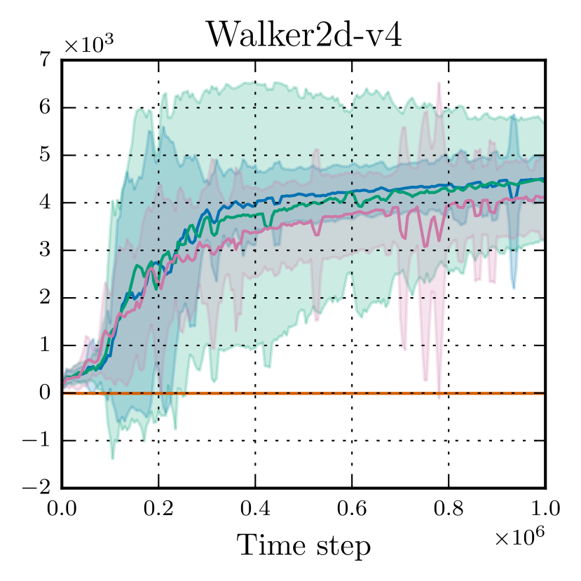
We evaluate the proposed methods on four of the eleven MuJoCo environments, namely Ant-v4, HalfCheetah-v4, Hopper-v4 and Walker2d-v4 (see Fig. 1). The goal is to walk as fast as possible without falling while at the same time minimizing the number of actions and reducing the impact on each joint. Observations consist of coordinate values of different robot’s body parts, followed by the velocities of each of those individual parts. Actions, bounded to $[-1,1]$, represent the torques applied at the joints. The dimensionality of both the observation and the action space varies across the environments, depending on the complexity of the task (see Table 1).

Hyperparameter values are reported in Table 2. We use the same architecture for both the policy and the action value network, consisting of $2$ fully connected hidden layers with ReLU nonlinearities. The action value network receives as an input the concatenation of the flattened observation and action and returns a Q-value. The policy network receives as an input the flattened observation and returns the parameters of the corresponding action distribution. In particular, for SAC-Beta-AD and SAC-Beta-OMT, it returns the logarithm of the concentration parameters shifted by $1$ to ensure that the distribution is both concave and unimodal Chou et al. (2017). For SAC-Normal and SAC-TanhNormal, it returns the mean and the logarithm of the standard deviation. For all distributions, we assume the action dimensions are independent. To improve training stability, we clip the log shifted concentrations and log standard deviation to the interval $[-20,2]$. Furthermore, we clip the samples drawn from the beta distribution to the interval $[10^{-7},1-10^{-7}]$ to avoid underflow and we linearly map them from $[0,1]$ to the environment’s action interval $[-1,1]$. We train the policy for $10^{6}$ time steps using Adam optimizer Kingma and Ba (2015) with a learning rate of $0.001$ and a batch size of $256$. We perform $1$ gradient update per time step and synchronize the target networks after each update with smoothing coefficient $0.005$. We use a discount factor of $0.99$, a temperature of $0.2$ and a replay buffer of size $10^{6}$, which is filled with $10^{4}$ initial transitions collected by sampling actions uniformly at random. We test the policy every $5000$ time steps for $10$ episodes using the distribution mean as the predicted action and we report the average return.

Software for the experimental evaluation was implemented in Python 3.10.2 using Gymnasium 0.28.1¹¹1https://github.com/Farama-Foundation/Gymnasium/tree/v0.28.1 Brockman et al. (2016) + EnvPool 0.8.1²²2https://github.com/sail-sg/envpool/tree/v0.8.1 Weng et al. (2022b) for the MuJoCo environments, Tianshou 0.5.0³³3https://github.com/thu-ml/tianshou/tree/v0.5.0 Weng et al. (2022a) for SAC, PyTorch 1.13.1⁴⁴4https://github.com/pytorch/pytorch/tree/v1.13.1 Paszke et al. (2019) for the neural network architectures, probability distributions and reference implementation of optimal mass transport implicit reparameterization, TensorFlow 2.11.0⁵⁵5https://github.com/tensorflow/tensorflow/tree/v2.11.0 Abadi et al. (2015) + TensorFlow Probability 0.19.0⁶⁶6https://github.com/tensorflow/probability/tree/v0.19.0 Dillon et al. (2017) for the reference implementation of automatic differentation implicit reparameterization and Matplotlib 3.7.0⁷⁷7https://github.com/matplotlib/matplotlib/tree/v3.7.0 Hunter (2007) for plotting. All the experiments were run on a CentOS Linux 7 machine with an Intel Xeon Gold 6148 Skylake CPU with $20$ cores @ $2.40$ GHz, $32$ GB RAM and an NVIDIA Tesla V100 SXM2 @ $16$ GB with CUDA Toolkit 11.4.2.

A comparison between the proposed SAC variants is presented in Fig. 1, with the final performance reported in Table 3. We observe that SAC-Normal struggles to learn anything useful, as the average return remains close to zero in all the environments. This could be ascribed to a poor initialization, as the training process immediately diverges and the policy gets stuck in a region of the search space from which it cannot recover. Further investigations are needed to understand why the normal policy performs poorly with SAC while it does not exhibit the same flawed behavior with other non-entropy-based algorithms such as TRPO Schulman et al. (2015); Chou et al. (2017). Overall, SAC-Beta-AD and SAC-Beta-OMT perform similarly to SAC-TanhNormal, with slightly higher final return in Ant-v4 and Walker2d-v4 but worse in HalfCheetah-v4 and Hopper-v4. However, the large standard deviation values indicate that more experiments might be necessary to obtain more accurate estimates. Regarding the comparison between SAC-Beta-AD and SAC-Beta-OMT, we only observe little differences mostly due to random fluctuations. This is surprising, since we were expecting faster convergence with SAC-Beta-AD, given the fact that it provides more accurate gradient estimates Figurnov et al. (2018). This suggests that highly accurate gradients may not be critical to the algorithm’s success. Therefore, a simpler gradient estimator such as the score function estimator Mohamed et al. (2020), which does not rely on assumptions about the distribution family, could be a promising alternative to explore.

We also conduct an ablation study for SAC-Beta-OMT on Ant-v4 to gain more insights on the impact of our design choices. In particular, we consider the following three ablations:

• •

  SAC-Beta-OMT-no_clip: we do not clip the log shifted concentrations.

• •

  SAC-Beta-OMT-non_concave: we do not shift the concentrations, allowing for non-concave beta distributions.

• •

  SAC-Beta-OMT-softplus: following Chou et al. (2017), we model the concentrations using $\operatorname{softplus}$ instead of $\exp$, meaning that the policy network effectively returns inverse softplus shifted concentrations.

As depicted in Fig. 2, SAC-Beta-OMT performs the best, demonstrating the effectiveness of our training setup. Note that SAC-Beta-OMT-no_clip terminates prematurely after $\sim 400$ k time steps due to exploding or vanishing concentrations, leading us to the conclusion that clipping is crucial to avoid instabilities in the optimization process.

References

- Abadi et al. [2015] M. Abadi, A. Agarwal, P. Barham, E. Brevdo, Z. Chen, C. Citro, G. S. Corrado, A. Davis, J. Dean, M. Devin, S. Ghemawat, I. Goodfellow, A. Harp, G. Irving, M. Isard, Y. Jia, R. Jozefowicz, L. Kaiser, M. Kudlur, J. Levenberg, D. Mané, R. Monga, S. Moore, D. Murray, C. Olah, M. Schuster, J. Shlens, B. Steiner, I. Sutskever, K. Talwar, P. Tucker, V. Vanhoucke, V. Vasudevan, F. Viégas, O. Vinyals, P. Warden, M. Wattenberg, M. Wicke, Y. Yu, and X. Zheng. TensorFlow: Large-scale machine learning on heterogeneous systems, 2015. URL https://www.tensorflow.org.
- Bhattacharjee [1970] G. P. Bhattacharjee. Algorithm AS 32: The incomplete gamma integral. Journal of the Royal Statistical Society. Series C (Applied Statistics), 19(3):285–287, 1970. URL https://www.jstor.org/stable/2346339.
- Brockman et al. [2016] G. Brockman, V. Cheung, L. Pettersson, J. Schneider, J. Schulman, J. Tang, and W. Zaremba. OpenAI Gym. arXiv preprint arXiv:1606.01540v1, 2016. URL http://arxiv.org/abs/1606.01540v1.
- Chou et al. [2017] P.-W. Chou, D. Maturana, and S. Scherer. Improving stochastic policy gradients in continuous control with deep reinforcement learning using the beta distribution. In International Conference on Machine Learning (ICML), volume 70, pages 834–843, 2017. URL https://proceedings.mlr.press/v70/chou17a.html.
- Dillon et al. [2017] J. V. Dillon, I. Langmore, D. Tran, E. Brevdo, S. Vasudevan, D. Moore, B. Patton, A. Alemi, M. D. Hoffman, and R. A. Saurous. TensorFlow Distributions. arXiv preprint arXiv:1711.10604v1, 2017. URL https://arxiv.org/abs/1711.10604v1.
- Dinh et al. [2017] L. Dinh, J. Sohl-Dickstein, and S. Bengio. Density estimation using Real NVP. In International Conference on Learning Representations, (ICLR), 2017. URL https://arxiv.org/abs/1605.08803v3.
- Figurnov et al. [2018] M. Figurnov, S. Mohamed, and A. Mnih. Implicit reparameterization gradients. In International Conference on Neural Information Processing Systems (NeurIPS), volume 31, 2018. URL https://arxiv.org/abs/1805.08498v4.
- Haarnoja et al. [2018] T. Haarnoja, A. Zhou, P. Abbeel, and S. Levine. Soft actor-critic: Off-policy maximum entropy deep reinforcement learning with a stochastic actor. In International Conference on Machine Learning (ICML), pages 1861–1870, 2018. URL https://arxiv.org/abs/1801.01290v2.
- Hasselt et al. [2016] H. V. Hasselt, A. Guez, and D. Silver. Deep reinforcement learning with double Q-learning. In AAAI Conference on Artificial Intelligence, pages 2094–2100, 2016. URL https://arxiv.org/abs/1509.06461v3.
- Hunter [2007] J. D. Hunter. Matplotlib: A 2D graphics environment. Computing in Science & Engineering, 9(3):90–95, 2007. URL https://doi.org/10.1109/MCSE.2007.55.
- Jankowiak and Obermeyer [2018] M. Jankowiak and F. Obermeyer. Pathwise derivatives beyond the reparameterization trick. In International Conference on Machine Learning (ICML), volume 80, pages 2240–2249, 2018. URL https://arxiv.org/abs/1806.01851v2.
- Kingma and Ba [2015] D. P. Kingma and J. Ba. Adam: A method for stochastic optimization. In International Conference on Learning Representations (ICLR), 2015. URL https://arxiv.org/abs/1412.6980v9.
- Mazoure et al. [2020] B. Mazoure, T. Doan, A. Durand, J. Pineau, and R. D. Hjelm. Leveraging exploration in off-policy algorithms via normalizing flows. In Conference on Robot Learning (CoRL), pages 430–444, 2020. URL https://arxiv.org/abs/1905.06893v3.
- Mnih et al. [2013] V. Mnih, K. Kavukcuoglu, D. Silver, A. Graves, I. Antonoglou, D. Wierstra, and M. Riedmiller. Playing atari with deep reinforcement learning. In International Conference on Neural Information Processing Systems (NeurIPS), 2013. URL https://arxiv.org/abs/1312.5602v1.
- Mnih et al. [2015] V. Mnih, K. Kavukcuoglu, D. Silver, A. A. Rusu, J. Veness, M. G. Bellemare, A. Graves, M. A. Riedmiller, A. K. Fidjeland, G. Ostrovski, S. Petersen, C. Beattie, A. Sadik, I. Antonoglou, H. King, D. Kumaran, D. Wierstra, S. Legg, and D. Hassabis. Human-level control through deep reinforcement learning. Nature, pages 529–533, 2015. URL https://doi.org/10.1038/nature14236.
- Mohamed et al. [2020] S. Mohamed, M. Rosca, M. Figurnov, and A. Mnih. Monte carlo gradient estimation in machine learning. Journal of Machine Learning Research (JMLR), 21(1), 2020. URL https://arxiv.org/abs/1906.10652v2.
- Paszke et al. [2019] A. Paszke, S. Gross, F. Massa, A. Lerer, J. Bradbury, G. Chanan, T. Killeen, Z. Lin, N. Gimelshein, L. Antiga, A. Desmaison, A. Kopf, E. Yang, Z. DeVito, M. Raison, A. Tejani, S. Chilamkurthy, B. Steiner, L. Fang, J. Bai, and S. Chintala. PyTorch: An imperative style, high-performance deep learning library. In International Conference on Neural Information Processing Systems (NeurIPS), volume 32, 2019. URL https://arxiv.org/abs/1912.01703v1.
- Rezende and Mohamed [2015] D. Rezende and S. Mohamed. Variational inference with normalizing flows. In International Conference on Machine Learning (ICML), volume 37, pages 1530–1538, 2015. URL https://arxiv.org/abs/1505.05770v6.
- Schulman et al. [2015] J. Schulman, S. Levine, P. Abbeel, M. Jordan, and P. Moritz. Trust region policy optimization. In International Conference on Machine Learning (ICML), pages 1889–1897, 2015. URL https://arxiv.org/abs/1502.05477v5.
- Schulman et al. [2016] J. Schulman, P. Moritz, S. Levine, M. Jordan, and P. Abbeel. High-dimensional continuous control using generalized advantage estimation. In International Conference on Learning Representations (ICLR), 2016. URL https://arxiv.org/abs/1506.02438v6.
- Silver et al. [2016] D. Silver, A. Huang, C. J. Maddison, A. Guez, L. Sifre, G. van den Driessche, J. Schrittwieser, I. Antonoglou, V. Panneershelvam, M. Lanctot, S. Dieleman, D. Grewe, J. Nham, N. Kalchbrenner, I. Sutskever, T. Lillicrap, M. Leach, K. Kavukcuoglu, T. Graepel, and D. Hassabis. Mastering the game of Go with deep neural networks and tree search. Nature, 529:484–489, 2016. URL https://doi.org/10.1038/nature16961.
- Sutton [1988] R. S. Sutton. Learning to predict by the methods of temporal differences. Machine Learning, pages 9–44, 1988. URL https://doi.org/10.1023/A:1022633531479.
- Sutton and Barto [1998] R. S. Sutton and A. G. Barto. Reinforcement Learning: An Introduction. MIT Press, 1998.
- Todorov et al. [2012] E. Todorov, T. Erez, and Y. Tassa. MuJoCo: A physics engine for model-based control. In IEEE/RSJ International Conference on Intelligent Robots and Systems, pages 5026–5033, 2012. URL https://doi.org/10.1109/IROS.2012.6386109.
- Wang et al. [2017] Z. Wang, V. Bapst, N. Heess, V. Mnih, R. Munos, K. Kavukcuoglu, and N. de Freitas. Sample efficient actor-critic with experience replay. In International Conference on Learning Representations (ICLR), 2017. URL https://arxiv.org/abs/1611.01224v2.
- Ward et al. [2019] P. Ward, A. Smofsky, and A. Bose. Improving exploration in soft-actor-critic with normalizing flows policies. In International Conference on Machine Learning (ICML), 2019. URL https://arxiv.org/abs/1906.02771v1.
- Weng et al. [2022a] J. Weng, H. Chen, D. Yan, K. You, A. Duburcq, M. Zhang, Y. Su, H. Su, and J. Zhu. Tianshou: A highly modularized deep reinforcement learning library. Journal of Machine Learning Research (JMLR), 23(267):1–6, 2022a. URL https://arxiv.org/abs/2107.14171v3.
- Weng et al. [2022b] J. Weng, M. Lin, S. Huang, B. Liu, D. Makoviichuk, V. Makoviychuk, Z. Liu, Y. Song, T. Luo, Y. Jiang, Z. Xu, and S. Yan. EnvPool: A highly parallel reinforcement learning environment execution engine. In International Conference on Neural Information Processing Systems (NeurIPS), volume 35, pages 22409–22421, 2022b. URL https://arxiv.org/abs/2206.10558v2.