\addauthor

tlcyan \addauthoradolive \addauthorjbmagenta

Social Learning with Bounded Rationality:
Negative Reviews Persist under Newest First

Jackie Baek Stern School of Business, New York University, [email protected] Atanas Dinev Massachusetts Institute of Technology, [email protected] Thodoris Lykouris Massachusetts Institute of Technology, [email protected]

(First version: June 2024
Current version: August 2024¹¹1An extended abstract appeared at the ACM Conference on Economics and Computation (EC) 2024.)

Abstract

We study a model of social learning from reviews where customers are computationally limited and make purchases based on reading only the first few reviews displayed by the platform. Under this bounded rationality, we establish that the review ordering policy can have a significant impact. In particular, the popular Newest First ordering induces a negative review to persist as the most recent review longer than a positive review. This phenomenon, which we term the Cost of Newest First, can make the long-term revenue unboundedly lower than a counterpart where reviews are exogenously drawn for each customer.

We show that the impact of the Cost of Newest First can be mitigated under dynamic pricing, which allows the price to depend on the set of displayed reviews. Under the optimal dynamic pricing policy, the revenue loss is at most a factor of 2. On the way, we identify a structural property for this optimal dynamic pricing: the prices should ensure that the probability of a purchase is always the same, regardless of the state of reviews. We also study an extension of the model where customers put more weight on more recent reviews (and discount older reviews based on their time of posting), and we show that Newest First is still not the optimal ordering policy if customers discount slowly.

Lastly, we corroborate our theoretical findings using a real-world review dataset. We find that the average rating of the first page of reviews is statistically significantly smaller than the overall average rating, which is in line with our theoretical results.

1 Introduction

The use of product reviews to inform customer purchase decisions has become ubiquitous in a variety of online platforms, ranging from electronic commerce to accommodation and recommendation platforms. While the online nature of such platforms may hinder the ability of customers to confidently evaluate the product compared to an in-person experience, reviews written by previous customers can shed light on the product’s quality. It is well established that product reviews play a significant role on customer purchase decisions [CM06, ZZ10, Luc16].

The process in which reviews impact product purchases can be seen as a problem of social learning, which generically studies how agents update their beliefs for an unknown quantity of interest (e.g., product quality) based on observing actions of past agents (e.g., reading reviews written by past customers). The typical assumption in the literature of social learning with reviews is that, when deciding whether to purchase a product, customers consider either all reviews provided by previous customers [CIMS17, IMSZ19, GHKV23] or a summary statistic such as their average rating [BS18, CLT21, AMMO22]. The motivation for the latter assumption is that customers have limited time and computational power and thus rely on a summary statistic, often provided by the platform (see Section 1.2 for a further discussion on these lines of work).

However, in practice, a common scenario may be somewhere “in between” the above two assumptions: customers read a small number of reviews in detail. Existing works have found that the textual content of a review contains important information that goes beyond its numeric score and such information can heavily influence purchase decisions [GI10, AGI11, LDRF⁺13, LLS19, LYMZ22]. Therefore, customers look beyond the average review rating and read a small number of reviews in detail. In particular, [Kav21] find that 76% of customers read between 1 and 9 reviews before making a purchase. This motivates the main questions of our work:

When customers read a limited number of reviews, how does this impact social learning?
Are there operational decisions that should be reconsidered due to this bounded rationality?

To answer these questions, we study a model for a single product (formalized in Section 2), where a platform makes decisions regarding how reviews are ordered and how the product is priced. Customers arrive sequentially and each customer takes only the first $c$ reviews into account to inform their purchase decision, where $c$ is a small constant. We assume that the $t$ ’th customer’s valuation can be decomposed as the sum of a) an idiosyncratic valuation $\Theta_{t}$ that is known to them and b) a product quality $\mu_{t}$ that has a fixed mean $\mu$ ; the latter quantity is unknown to the customer and can only be inferred via the reviews. We assume that when a customer reads a review written by customer $s$ , they observe $\mu_{s}$ (see Section 1.2 for a discussion of this assumption). Each customer uses $c$ reviews to update their belief about $\mu$ , and makes a purchase if their estimate of their valuation is higher than the price. In the event of a purchase, they leave a review that future customers can read.

1.1 Our contribution

A popular review ordering policy is to display reviews in reverse chronological order (newest to oldest); we refer to this policy as ${\sigma^{\textsc{newest}}}$ . This is the default option in platforms such as Airbnb, Tripadvisor and Macy’s²²2This statement is based on access on Feb 7, 2024. Many other platforms such as Amazon and Yelp list newest as the second default and have their own ordering mechanism as the default option. as it allows customers to get access to the most up-to-date reviews. In the context of our model, under the ${\sigma^{\textsc{newest}}}$ ordering, a customer considers the $c$ most recent reviews. The set of these $c$ reviews evolves as a stochastic process over customer arrivals: when a new purchase happens and thus a new review is provided, this review replaces the $c$ -th most recent review.

Cost of Newest First.

By analyzing the steady state of the aforementioned stochastic process, we observe that the ${\sigma^{\textsc{newest}}}$ ordering policy induces an undesirable behavior where negative reviews are read more than positive reviews, leading to a significant loss in overall revenue (Section 3).

To illustrate this phenomenon, consider a simple setting where customers only read the first review ( $c=1$ ) and the probability of a purchase is higher when the review is positive. When the $t$ ’th customer arrives, if the first review is positive, this customer is likely to buy the product and subsequently leave a review; the new review from the $t$ ’th customer then becomes the “first review” for the $(t+1)$ ’th customer. On the other hand, if the first review is negative for the $t$ ’th customer, they are less likely to buy the product, and hence the same negative review remains as the “first review” for the $(t+1)$ ’th customer. Therefore, negative reviews persist under the newest first ordering: a review will stay longer as the first review if it is negative compared to if it is positive.

We show that this arises due to the endogeneity of the stochastic process that ${\sigma^{\textsc{newest}}}$ induces and results in a loss of long-term revenue. To formalize this notion, we compare ${\sigma^{\textsc{newest}}}$ to an exogenous process where each arriving customer sees an independently drawn random set of reviews; we refer to this ordering policy as ${\sigma^{\textsc{random}}}$ . We establish that the long-term revenue under ${\sigma^{\textsc{newest}}}$ is strictly smaller than that of ${\sigma^{\textsc{random}}}$ under any non-degenerate instance (Theorem 3.1) and that the revenue under ${\sigma^{\textsc{newest}}}$ can be arbitrarily smaller, in a multiplicative sense, compared to ${\sigma^{\textsc{random}}}$ (Theorem 3.2). We refer to this phenomenon as the Cost of Newest First (CoNF).

Dynamic pricing mitigates CoNF.

Seeking to mitigate this phenomenon, we consider the impact of optimizing the product’s price (Section 4). We show that even under the optimal static price, the CoNF remains arbitrarily large (Theorem 4.1). However, if we allow for dynamic pricing, where the price can depend on the state of the reviews, we show that the CoNF is upper bounded by a factor of $2$ when the idiosyncratic valuation distribution is non-negative and gracefully decays with its negative mass otherwise (Theorem 4.2).

This improvement stems from the fact that dynamic pricing allows us to change the steady state distribution of the stochastic process. Recall that, under ${\sigma^{\textsc{newest}}}$ , the stochastic process spends more time on states with negative reviews than states with positive reviews. The optimal dynamic pricing policy sets prices so that the purchase probability is equal across all states (Theorem 4.4) — this ensures that the steady state distribution under ${\sigma^{\textsc{newest}}}$ is the same as that of ${\sigma^{\textsc{random}}}$ .

A broader implication of this result is that, when purchase decisions depend on the state of the first reviews, platforms that offer state-dependent prices can be arbitrarily better off than platforms that are unaware of this phenomenon and statically optimize prices (Theorem 4.6).

Time-discounting customers.

Having identified the potential inefficiency of the ${\sigma^{\textsc{newest}}}$ ordering policy, we extend our model to incorporate the main reason behind its popularity: customers often prefer to read more recent reviews as they contain more up-to-date content. A recent survey [Mur19] shows that $48\%$ of the participants only look at reviews within the last two weeks and over $85\%$ of the participants disregard any review that was not posted in the past three months.

To capture this recency-awareness, we extend our model to allow for customers to place more weight on more recent reviews when they update their beliefs (Section 5). Despite the presence of CoNF, when customers severely time-discount, we show that ${\sigma^{\textsc{newest}}}$ yields the highest revenue (Theorem 5.1); in the other extreme where customers do not discount at all, ${\sigma^{\textsc{random}}}$ maximizes revenue (Theorem 5.2). Interestingly, when customers discount slightly, neither of ${\sigma^{\textsc{newest}}}$ or ${\sigma^{\textsc{random}}}$ maximizes revenue; it is better to consider a finite window of the most recent $w$ reviews, and select $c$ reviews at random from this set (Theorem 5.3). Finally, we show that the CoNF interacts with the discount factor in a non-trivial way. For a random set of reviews, if higher weights imply a higher purchase probability, then one would expect that non-discounting customers purchase more than discounting customers. However, due to the CoNF, we show that there are cases in which discounting customers yield a higher purchase rate than non-discounting customers (Theorem 5.4).

Empirical evidence from Tripadvisor data.

Finally in Section 6, we corroborate our theoretical findings using real-world review data from Tripadvisor, an online platform where the default review ordering policy is newest first. We evaluate 109 hotel pages, and we find that for 79 of them, the average review rating of the first 10 reviews is lower than the average review rating of all reviews. These empirical findings support our main theoretical results with statistical significance.

1.2 Related Work and Comparison of Key Modeling Assumptions

Social learning and incentivized exploration.

Classical models of social learning from [Ban92] and [BHW92] study a setting in which there is an unknown state of the world and each agent observes an independent, noisy signal about the state as well as the actions of past agents. The agent uses this information to update their beliefs and then takes an action. In this setting, undesirable “herding” behavior can arise: agents may converge to taking the wrong action. Conceptually closer to our work, [Say18] shows that dynamic pricing can mitigate the aforementioned herding behavior. Subsequent works study how social learning is affected by the agent’s signal distribution [SS00], prior for the state [CDO22], heterogeneous preferences [GPR06, LS16], as well as the structure of their observations [AMMO22]. From a different perspective, there is a stream of literature that aim to design mechanisms to help the learning process, either by modifying the information structure [KMP14, MSS20, BPS18] or by incentivizing exploration through payments [FKKK14, KKM⁺17].

Social learning with reviews.

Closer to our work, several papers focus on the setting where customers learn about a product’s quality through reviews [HPZ17, CIMS17, BS18, SR18, IMSZ19, CLT21, AMMO22, GHKV23, Bon23, CSS24]. This literature induces several modeling differences compared to classical social learning. First, agents do not receive independent signals of the unknown state (the product quality). Second, agents not only observe the binary purchase decision of previous agents, but also the reviews of previous agents who purchased the product. We highlight the key modeling assumptions of our work and how they relate to existing works.

No self-selection bias.

In prior works of social learning with reviews, the main difficulty stems from the self-selection bias, the idea that only customers who value the product highly will buy the product and hence these customers leave reviews with higher ratings. In the presence of self-selection bias, [CIMS17] and [IMSZ19] study conditions in which customer beliefs eventually successfully learn the quality of a product, where customers update their beliefs based on the entire history of reviews. [AMMO22, BS18, SR18, CLT21] consider models in which customers only incorporate summary statistics of prior reviews (e.g., average rating) into their beliefs. [Bon23] analyzes how the magnitude of the self-selection bias depends on the product’s quality and polarization. [CSS24] consider a model where the platform’s pricing decision affect the review ratings and characterizes the impact of the price on the average rating. This is also empirically supported by [BMZ12] which shows that Groupon discounts lead to lower ratings. [HPZ17] study a two-stage model which quantifies both self-selection bias and under-reporting bias (reviews are provided only by customers with extreme experiences); see references within for further related work.

In contrast, our work studies a model where self-selection bias does not arise. Specifically, we assume that customer $t$ ’s valuation can be decomposed as $V_{t}=\Theta_{t}+\mu_{t}$ , where $\Theta_{t}$ is customer-specific, and $\mu_{t}$ has a fixed mean $\mu$ shared across customers. The quantity $\mu$ is the unknown quantity of interest for all customers. Our model assumes that a review reveals $\mu_{t}$ . In contrast, prior works assume that a review reveals $\Theta_{t}+\mu_{t}$ and one cannot separate the contribution from each term. This means that, in our model, the customer-specific valuation and the pricing decision affect the purchase probability but do not affect the review itself conditioning on a purchase. Although our assumption makes it “easier” for customers to learn $\mu$ , we study a new phenomenon that arises due to the fact that customers only read a small number of reviews.

The practical motivation for our modeling assumption is the following. On most online platforms, a review is composed by both a numeric score (e.g., 4 out of 5) and a textual description that further explains the reviewer’s thoughts. Within our model, one interpretation is that the numeric score reveals $\Theta_{t}+\mu_{t}$ , but one can use the textual content of the review to separate $\Theta_{t}$ from $\mu_{t}$ . Therefore, we assume that reading the text of the review reveals $\mu_{t}$ , but we also assume that each customer only reads a small number of reviews since reading the text takes time. Even though most platforms provide the average score of the numeric ratings, this will suffer from self-selection bias (as shown in [BS18, CLT21]) and hence customers must read reviews in detail to learn $\mu$ .

[GHKV23] also study a setting with no self-selection bias (without bounded rationality), focusing on dynamic pricing. Their model assumes that customers are partitioned into a finite number of types and only read reviews written by customers of the same type. This overcomes self-selection bias as customers of the same type can be thought of as having the same value of $\Theta_{t}$ in our model.

Belief convergence vs. stochastic process.

In the existing literature, social learning is deemed “successful” if the customer’s estimate of product quality converges to the true quality. This convergence can either be that their belief distribution converges to a single point [IMSZ19, AMMO22], or that the customer’s scalar estimate of the product quality (e.g., average rating) converges to the true quality [CIMS17, BS18]. In our setting, customers update their beliefs based on the first $c$ reviews and, as discussed above, these $c$ reviews evolve across customers as a stochastic process. Therefore, customer beliefs do not converge but rather oscillate based on the state of those $c$ reviews, even as the number of customers goes to infinity.

Closer to our work, [PSX21] study a similar model (without bounded rationality) and show that the initial review can have an effect on the proclivity of customer purchases and the number of reviews. This bias introduced by initial reviews is also empirically observed by the work of [LKAK18]. Unlike our model, this effect diminishes over time as the product acquires more reviews and the initial review becomes less salient. Our results on the Cost of Newest First can thus be viewed as a stronger version of the result in [PSX21] as we show that, in the presence of bounded rationality, the effect of negative reviews persists even in the steady-state of the system.

Fully Bayesian vs. non-Bayesian.

Existing papers differ in whether customers incorporate information from reviews in a fully Bayesian or non-Bayesian manner. For example, [IMSZ19] and [AMMO22] study a fully Bayesian setting where all distributions (prior on $\mu$ , distribution of $\Theta_{t}$ ) and purchasing behaviors are common knowledge and each customer forms a posterior belief on $\mu$ using the information given to them. In contrast, [CIMS17] and [CLT21] assume that customers use a simple non-Bayesian rule when making their purchase decision. Moreover, [BS18] study both Bayesian and non-Bayesian update rules and compare them.

In our paper, customers use a Bayesian framework but their update rule is not fully Bayesian. Specifically, customers start with a Beta prior on $\mu$ . This prior need not be correct as we assume that $\mu$ is a fixed number. We assume reviews are binary (0 or 1), and customers read $c$ of them and update their beliefs assuming that these reviews are independent draws from $Bernoulli(\mu)$ . However, this is not necessarily the “correct” Bayesian update rule for the customers, due to the endogeneity of the stochastic process of the first $c$ reviews. That is, under the ${\sigma^{\textsc{newest}}}$ ordering rule, negative reviews are more likely to persist as the most recent review — hence even if $\mu=1/2$ , the most recent review is more likely to be negative than positive. Therefore, a fully Bayesian customer should take this phenomenon into account when updating their beliefs. We assume that customers do not account for this (and hence are not fully Bayesian), and we study the impact of how this endogeneity impacts the steady state of the process. Our model also implicitly assumes that customers do not use additional information about previous customers’ non-purchase decisions (which are typically non-observable) and the platform’s pricing policy (which is often opaque).

Finally, our model is flexible in that it allows customers to map their belief distribution to a scalar estimate of $\mu$ in an arbitrary manner, e.g, the mean of the belief distribution (which is considered in most prior work) as well as a pessimistic estimate thereof (as studied in [GHKV23]).

Other work on social learning with reviews.

[HC24] study the design of rating systems motivated by the idea that older reviews become less relevant. In a setting where the product’s quality changes, they show that a moving average rating system is optimal in reflecting the true quality. Social learning with reviews has also been studied for ranking [MSSV23], incorporating quality variability [DLT21], dealing with non-stationary environments [BPS22], and has been applied to green technology adoption [RHP23].

2 Model

We consider a platform that repeatedly offers a product to customers that arrive in consecutive rounds $t=1,2,\ldots$ . The customer makes a purchase decision based on a finite number of reviews and the price; if a purchase occurs, they leave a new review for the product. We consider the platform’s decisions regarding the ordering of reviews as well as the price.

Customer valuation. The customer at round $t$ has a realized valuation $V_{t}=\mu_{t}+\Theta_{t}\in\mathbb{R}$ for the product, where $\mu_{t}$ and $\Theta_{t}$ represent the contribution from the product’s unobservable and observable parts respectively. Specifically, $\mu_{t}\in\{0,1\}$ is drawn independently from $Bernoulli(\mu)$ for each customer $t$ , where $\mu\in(0,1)$ is the same across all customers and is unknown to them. Contrastingly, the quantity $\Theta_{t}$ is customer-specific and is known to customer $t$ before they purchase. We assume that, at every round $t$ , $\Theta_{t}$ is drawn independently from a distribution $\mathcal{F}$ with bounded support. The platform knows the distribution $\mathcal{F}$ but not $\Theta_{t}$ .

If the customer at round $t$ knew their exact valuation $V_{t}$ , then they would purchase the product if and only if $V_{t}\geq p_{t}$ , where $p_{t}$ is the price of the product at time $t$ . However, $\mu_{t}$ is unknown and hence so is $V_{t}$ . We assume that the customers read reviews to learn about $\mu$ , and their purchase decision depends on their belief about $\mu$ after reading the reviews. Note that customers cannot aim to estimate $\mu_{t}$ beyond estimating $\mu$ , since $\mu_{t}$ is drawn independently for each customer.

Review generation. If the customer at round $t$ purchases the product, they write a review that future customers may read. The review rating given by customer $t$ is $\mu_{t}\in\{0,1\}$ (see Section 1.2 for a discussion of this assumption). We often refer to a review with $\mu_{t}=1$ as positive and to a review with $\mu_{t}=0$ as negative. We denote by $X_{t}\in\{0,1,\perp\}$ the rating of customer $t$ ’s review, where $X_{t}=\perp$ if customer $t$ did not purchase the product.

2.1 Customer Purchase Behavior

We describe the customer purchase behavior at one round, taking the price and the review ordering as fixed. Customers have a prior $\mathrm{Beta}(a,b)$ for the value of $\mu$ , for some fixed $a,b>0$ . This prior need not be correct and could be based on information about the features of the product or summary statistics of all reviews which are subject to self-selection bias (see discussion in Section 1.2). Customers read the first $c$ reviews that are shown to them to update their prior. Formally, letting $\bm{Z}_{t}=(Z_{t,1},\ldots,Z_{t,c})\in\{0,1\}^{c}$ denote the ratings of the first $c$ reviews shown, the customer creates the following posterior for the unobservable quality $\mu$ :

\Phi_{t}\coloneqq\mathrm{Beta}\left(a+\sum_{i=1}^{c}Z_{t,i},b+c-\sum_{i=1}^{c}Z_{t,i}\right).

This corresponds to the natural posterior update for $\mu$ if each $Z_{t,i}$ is an independent draw from $Bernoulli(\mu)$ .³³3The reviews $\bm{Z}_{t}$ are not necessarily independent draws from $Bernoulli(\mu)$ , hence the customers are not completely Bayesian. See the last point in Section 1.2 for a detailed discussion. Note that the customer places equal weight on the first $c$ reviews (we also consider time-discounted weights in Section 5). Based on this posterior, the customer creates an estimate $\hat{V}_{t}$ for their valuation. We assume that there is a mapping $h(\Phi_{t})\in(0,1)$ from their posterior to a real number that represents an estimate of the fixed valuation $\mu$ . For example, the mapping $h(\Phi_{t})={\mathbb{E}}[\Phi_{t}]$ represents risk-neutral customers, while if $h(\Phi_{t})$ corresponds to the $\phi$ -quantile of $\Phi_{t}$ for $\phi<0.5$ , this represents pessimistic customers (see Section 5.1). The customer then forms their estimated valuation $\hat{V}_{t}\coloneqq\Theta_{t}+h(\Phi_{t})$ and buys the product at price $p_{t}$ if and only if $\hat{V}_{t}\geq p_{t}$ . Finally, the customer leaves a review $X_{t}\sim Bernoulli(\mu)$ if they bought the product, otherwise $X_{t}=\perp$ .

To ease exposition, we often use $n$ to denote the number of positive ratings (i.e., $n=\sum_{i=1}^{c}Z_{t,i}$ ), and we overload notation to denote by $h(n)$ to refer to $h(\mathrm{Beta}(a+n,b+c-n))$ . We make the natural assumption that higher number of positive ratings leads to a higher purchase probability.

Assumption 2.1.

The estimate $h(n)$ is strictly increasing in the number of positive reviews $n$ .

We also assume that the idiosyncratic valuation has positive mass on non-negative values.

Assumption 2.2.

The distribution $\mathcal{F}$ has positive mass on non-negative values: ${\mathbb{P}}_{\Theta\sim\mathcal{F}}[\Theta\geq 0]>0$ .

We denote the above problem instance as $\mathcal{E}(\mu,\mathcal{F},a,b,c,h)$ for product quality $\mu$ , prior parameters $a,b$ , idiosyncratic distribution $\mathcal{F}$ , customers’ attention budget $c$ , and an estimate mapping $h$ .

2.2 Platform Decisions

We consider two platform decisions, review ordering and pricing.

Review ordering. With respect to ordering, since customers only take the first $c$ reviews into account, choosing an ordering is equivalent to selecting a set of $c$ reviews to show. Let $I_{t}=\{\tau<t:X_{\tau}\neq\perp\}$ be the set of previous rounds in which a review was submitted and let $\mathcal{H}_{t}=\{I_{t},\{X_{\tau}\}_{\tau<t},\{p_{\tau}\}_{\tau<t},\{\bm{Z}_{\tau}\}_{\tau<t}\}$ be the observed history before round $t$ . At round $t$ , the platform maps (possibly in a randomized way) its observed history $\mathcal{H}_{t}$ to the set of review ratings $\sigma(\mathcal{H}_{t})$ corresponding to the $c$ reviews shown. We study the steady-state distribution of the system; to avoid initialization corner cases, we assume that at time $t=1$ , there is an infinite pool of reviews $\{X_{\tau}\}_{\tau=-\infty}^{-1}$ where $X_{\tau}\stackrel{{\scriptstyle\text{i.i.d.}}}{{\sim}}Bernoulli(\mu)$ . We consider the following review ordering policies:

•

$\sigma^{\textsc{newest}}$ selects the $c$ newest reviews. This is formally defined as $\sigma^{\textsc{newest}}(\mathcal{H}_{t})=(Z_{t,i})_{i=1}^{c}$ where $Z_{t,i}$ is the rating of the $i$ -th most recent review.
•

${\sigma^{\textsc{random}(w)}}$ selects $c$ reviews uniformly at random (without replacement) from the most recent $w\geq c$ reviews, independently at each round $t$ . Note that $\sigma^{\textsc{random}(c)}=\sigma^{\textsc{newest}}$ .
•

$\sigma^{\textsc{random}}$ shows $c$ random reviews. This corresponds to ratings being drawn independently from $Bernoulli(\mu)$ at each round $t$ ; i.e., $\sigma^{\textsc{random}}(\mathcal{H}_{t})=(Z_{t,i})_{i=1}^{c}$ where $Z_{t,i}\stackrel{{\scriptstyle\text{i.i.d.}}}{{\sim}}Bernoulli(\mu)$ .

Formally, $\sigma^{\textsc{random}}$ is defined as the limit of $\sigma^{\textsc{random}(w)}$ as $w\to\infty$ (see Appendix A for details). Note that, under $\sigma^{\textsc{random}}$ , the customers’ and platform’s actions at the current round do not influence the reviews shown in future rounds (i.e. the reviews are exogenous). In contrast, under $\sigma^{\textsc{newest}}$ and ${\sigma^{\textsc{random}(w)}}$ for any $w\in\mathbb{N}$ , the customers’ and platform’s actions influence what reviews are shown in future rounds (i.e. the reviews are endogenous to the underlying stochastic process).

Pricing. The platform also decides on the pricing policy, where the price at each round can depend on the set of $c$ displayed reviews. We denote a pricing policy by a function $\rho:\{0,1\}^{c}\to\mathbb{R}$ , which maps the set of displayed review ratings $\bm{z}\in\{0,1\}^{c}$ to a price. We study two classes of pricing policies: static and dynamic. We let $\Pi^{\textsc{static}}$ be the set of pricing policies $\rho$ that assign a fixed price $p$ , i.e., $\rho(\bm{z})=p$ for any $\bm{z}$ . Similarly, $\Pi^{\textsc{dynamic}}$ includes the set of pricing policies $\rho$ where $\rho(\bm{z})$ can depend on the review ratings $\bm{z}$ .

2.3 Revenue and the Cost of Newest First

For an ordering policy $\sigma$ and pricing policy $\rho$ , we define the revenue as the steady-state revenue:⁴⁴4The policies we consider have a stationary distribution so, in our analysis, we replace the $\liminf$ with a $\lim$ .

\textsc{Rev}(\sigma,\rho)\coloneqq\liminf_{T\to\infty}{\mathbb{E}}\Big{[}\frac{\sum_{t=1}^{T}\rho(\bm{Z}_{t})\mathbbm{1}_{\Theta_{t}+h(\Phi_{t})\geq\rho(\bm{Z}_{t})}}{T}\Big{]}.

(1)

Our main focus lies in understanding the effect of the ordering policy on the revenue. Specifically, we compare the revenues of the ordering policies $\sigma^{\textsc{newest}}$ and $\sigma^{\textsc{random}}$ . For a pricing policy $\rho$ , we define the Cost of Newest First (CoNF) as follows:⁵⁵5For all the policies $\rho$ we consider, $\textsc{Rev}(\sigma^{\textsc{newest}},\rho)>0$ . This is formalized for $\rho\in\Pi^{\textsc{static}}$ in Definition 3.1.

\chi(\rho)\coloneqq\frac{\textsc{Rev}(\sigma^{\textsc{random}},\rho)}{{\textsc{Rev}(\sigma^{\textsc{newest}},\rho)}}.

If $\rho\in\Pi^{\textsc{static}}$ , i.e., $\rho(\bm{z})=p$ for any $\bm{z}\in\{0,1\}^{c}$ we use $\textsc{Rev}(\sigma,p)$ and $\chi(p)$ as shorthand for the corresponding steady-state revenue and CoNF.

In Section 4, we study the CoNF when the platform can optimize its pricing policy over a class of policies. For a class of pricing policies $\Pi$ , we define similarly the optimal revenue within-class with respect to an ordering policy $\sigma$ and the corresponding CoNF as:

\textsc{Rev}(\sigma,\Pi)\coloneqq\sup_{\rho\in\Pi}\textsc{Rev}(\sigma,\rho)\qquad\text{and}\qquad\chi(\Pi)\coloneqq\frac{\textsc{Rev}(\sigma^{\textsc{random}},\Pi)}{\textsc{Rev}(\sigma^{\textsc{newest}},\Pi)}\qquad\text{respectively}.

To ease exposition, we make the mild assumption that $0<{\textsc{Rev}}(\sigma,\Pi)<\infty$ .⁶⁶6For the policies we consider, ${\textsc{Rev}}(\sigma,\Pi)>0$ by Assumption 2.2 and the fact that $h(0)>0$ ; ${\textsc{Rev}}(\sigma,\Pi)<\infty$ is satisfied if the maximum revenue from a customer’s idiosyncratic valuation is finite, i.e., $\sup_{p}p{\mathbb{P}}_{\Theta\sim\mathcal{F}}(\Theta\geq p)<+\infty$ .

Finally, we note that, unlike classical revenue maximization works, our focus is not on identifying policies that maximize revenue but rather in comparing the performance of different ordering policies ( $\sigma^{\textsc{newest}}$ vs $\sigma^{\textsc{random}}$ ) and different pricing policies ( $\Pi^{\textsc{static}}$ vs $\Pi^{\textsc{dynamic}}$ ).

Remark 2.1.

Our assumption of Bernoulli reviews and Beta prior is made for ease of exposition. Our results extend to a more general model where reviews come from an arbitrary distribution with finite support (not only $\{0,1\}$ ) and the estimator $h$ arbitrarily maps reviews to an estimate for the fixed valuation $\mu$ ; see Appendix B for details.

3 Cost of Newest First with a Fixed Static Price

Throughout this section, we assume a static pricing policy where the price $p$ is fixed and given. We establish the main phenomenon of the Cost of Newest First by showing that $\chi(p)>1$ under very mild conditions on the price $p$ . We then show that $\chi(p)$ can be arbitrarily large.

Recall that $h(n)$ refers to $h(\mathrm{Beta}(a+n,b+c-n))$ , where $n\in\{0,\ldots,c\}$ refers to the number of positive reviews. We first introduce two natural conditions that the price should satisfy.

Definition 3.1 (Non-absorbing price).

A price $p$ is non-absorbing if the purchase probability is positive for any displayed review ratings; i.e., for all $n\in\{0,1,\dots,c\}$ ,

{\mathbb{P}}_{\Theta\sim\mathcal{F}}[\Theta+h(n)\geq p]>0.

A non-absorbing price is required to guarantee that $\sigma^{\textsc{newest}}$ does not get “stuck” in a zero-revenue state. Specifically, under an absorbing price, there exists a set of review ratings such that the purchase probability is zero. In such a state, there will be no new subsequent review, and the set of most recent reviews will never be updated, resulting in zero revenue for $\sigma^{\textsc{newest}}$ . This is formalized in the following proposition (whose proof is provided in Appendix C.1).

Proposition 3.1.

Any absorbing price $p$ yields $0$ revenue under $\sigma^{\textsc{newest}}$ , i.e., ${\textsc{Rev}}(\sigma^{\textsc{newest}},p)=0$ .

Definition 3.2 (Non-degenerate price).

A price $p$ is non-degenerate if there exist $n_{1},n_{2}\in\{0,\ldots,c\}$ , $n_{1}\neq n_{2}$ such that the purchase probability is different given $n_{1}$ and $n_{2}$ positive review ratings:

{\mathbb{P}}_{\Theta\sim\mathcal{F}}[\Theta+h(n_{1})\geq p]\neq{\mathbb{P}}_{\Theta\sim\mathcal{F}}[\Theta+h(n_{2})\geq p].

A non-degenerate price implies that the review ratings “matter”, since there exist distinct review ratings where the purchase probability differs. In contrast, under a degenerate price, the review ratings have no impact on the purchase probability, hence the review ordering policy has no impact on revenue under such prices. Note that there exist prices which are absorbing and non-degenerate and there also exist prices which are degenerate and non-absorbing.⁷⁷7E.g. if $\mathcal{F}=\mathcal{U}[0,1]$ , $c=a=b=1$ , and $h(n)=\frac{n+1}{3}$ (mean). Then the price $p=\frac{4}{3}$ is non-degenerate but absorbing, while the price $p=\frac{1}{3}$ is degenerate but non-absorbing.

3.1 Existence of Cost of Newest First

Our main result is that the revenue under $\sigma^{\textsc{random}}$ is strictly higher than that of $\sigma^{\textsc{newest}}$ ; that is, $\chi(p)>1$ . As a building block towards this result, we first provide simple and interpretable closed form expressions for $\textsc{Rev}(\sigma^{\textsc{random}},p)$ and $\textsc{Rev}(\sigma^{\textsc{newest}},p)$ for a static price $p$ , which are given in Propositions 3.2 and 3.3 respectively. Let ${\mathrm{Bern}}(\mu)$ denote the Bernoulli distribution with success probability $\mu$ and ${\mathrm{Binom}}(c,\mu)$ denote the Binomial distribution with $c$ i.i.d. ${\mathrm{Bern}}(\mu)$ trials.

Proposition 3.2 (Revenue of $\sigma^{\textsc{random}}$ ).

For any fixed price $p$ ,

\textsc{Rev}(\sigma^{\textsc{random}},p)=p{\mathbb{E}}_{N\sim{\mathrm{Binom}}(c,\mu)}\Big{[}{\mathbb{P}}_{\Theta\sim\mathcal{F}}[\Theta+h(N)\geq p]\Big{]}.

Proof.

By definition, $\sigma^{\textsc{random}}$ displays $c$ i.i.d. ${\mathrm{Bern}}(\mu)$ reviews at every round $t$ . As a result, the number of positive reviews is distributed as ${\mathrm{Binom}}(c,\mu)$ , yielding expected revenue, at every round $t$ , equal to the right hand side of the theorem. Given that this quantity does not depend on $t$ , recalling Eq.(1), it equals the steady-state revenue. ∎

Unlike $\sigma^{\textsc{random}}$ which displays $c$ i.i.d. ${\mathrm{Bern}}(\mu)$ reviews at every round, the reviews displayed by $\sigma^{\textsc{newest}}$ are an endogenous function of the history. The proof of the next result underlies the technical crux of this section and is presented in Section 3.2.

Proposition 3.3 (Revenue of $\sigma^{\textsc{newest}}$ ).

For any non-absorbing fixed price $p$ ,

\textsc{Rev}(\sigma^{\textsc{newest}},p)=\frac{p}{{\mathbb{E}}_{N\sim{\mathrm{Binom}}(c,\mu)}\Big{[}\frac{1}{{\mathbb{P}}_{\Theta\sim\mathcal{F}}[\Theta+h(N)\geq p]}\Big{]}}.

Intuitively, when the newest reviews are positive, the customer is more likely to buy the product and leave a new review, which then updates the set of newest reviews. On the other hand, when the newest reviews are negative, the customer is less likely to buy, and hence the set of newest reviews is less likely to be updated. This implies that $\sigma^{\textsc{newest}}$ spends more time in a state with negative reviews (which yield lower revenue) compared to $\sigma^{\textsc{random}}$ . This phenomenon is the driver of our main result and we refer to it as the Cost of Newest First (CoNF).

Theorem 3.1 (Cost of Newest First).

For any non-degenerate price $p>0$ , the revenue of $\sigma^{\textsc{newest}}$ is strictly smaller than that of $\sigma^{\textsc{random}}$ , i.e., $\textsc{Rev}(\sigma^{\textsc{random}},p)>\textsc{Rev}(\sigma^{\textsc{newest}},p)$ .

Proof.

If $p$ is absorbing (Definition 3.1), by Proposition 3.1, $\textsc{Rev}(\sigma^{\textsc{newest}},p)=0$ as there is a state of reviews in which there will never be another purchase. However, $\textsc{Rev}(\sigma^{\textsc{random}},p)>0$ as $p$ is non-degenerate and hence there is a state of reviews with a positive purchase probability.

If $p$ is non-absorbing, we next show that the expression of Proposition 3.2 is higher than the one of Proposition 3.3. By Jensen’s inequality, ${\mathbb{E}}[X]\geq\frac{1}{{\mathbb{E}}[\frac{1}{X}]}$ for any non-negative random variable $X$ and equality is achieved if and only if $X$ is a constant. Letting $X(N)\coloneqq{\mathbb{P}}_{\Theta\sim\mathcal{F}}[\Theta+h(N)\geq p]$ be the purchase probability in a state with $N$ positive reviews, we apply the inequality for $X=X(N)$ ,

{\mathbb{E}}_{N\sim{\mathrm{Binom}}(c,\mu)}\big{[}{\mathbb{P}}_{\Theta\sim\mathcal{F}}[\Theta+h(N)\geq p]\big{]}\geq\frac{1}{{\mathbb{E}}_{N\sim{\mathrm{Binom}}(c,\mu)}\Big{[}\frac{1}{{\mathbb{P}}_{\Theta\sim\mathcal{F}}[\Theta+h(N)\geq p]}\Big{]}}.

Multiplying with $p>0$ on both sides we obtain that ${\textsc{Rev}}(\sigma^{\textsc{random}},p)\geq{\textsc{Rev}}(\sigma^{\textsc{newest}},p)$ . It remains to show that when $p$ is non-degenerate, the inequality is strict. Note that since $p$ is non-degenerate, we have that ${\mathbb{P}}_{\Theta\sim\mathcal{F}}[\Theta+h(0)\geq p]<{\mathbb{P}}_{\Theta\sim\mathcal{F}}[\Theta+h(c)\geq p]$ and thus ${\mathbb{P}}_{\Theta\sim\mathcal{F}}[\Theta+h(N)\geq p]$ is not a constant random variable when $N\sim{\mathrm{Binom}}(c,\mu)$ . Therefore, the inequality is strict. ∎

We describe a simple example that provides intuition on the CoNF established in Theorem 3.1, which is also illustrated in Figure 1.

Example 3.1.

Suppose $\mu=\frac{1}{2}$ , $\mathcal{F}=\mathcal{U}[0,1]$ , $c=a=b=1$ , $h(\Phi_{t})=\mathbb{E}[\Phi_{t}]=\frac{N+1}{3}$ , and $p=1$ . Under $\sigma^{\textsc{random}}$ the probability that the review shown is positive is $0.5$ (see Figure 1(a)). Under ${\sigma^{\textsc{newest}}}$ the purchase probability is $\frac{2}{3}$ when the review is positive and $\frac{1}{3}$ when it is negative. Thus, under $\sigma^{\textsc{newest}}$ , transitioning from a positive to a negative review is twice as likely as transitioning from a negative to a positive review (see Figure 1(b)). Hence, a negative rating is twice as likely as positive rating. This leads to lower revenue in steady state for $\sigma^{\textsc{newest}}$ compared to $\sigma^{\textsc{random}}$ .

(a)

\sigma^{\textsc{random}}

transitions.

(b)

\sigma^{\textsc{newest}}

transitions.

Figure 1: The state transitions in the instance of the Example 3.1 under

\sigma^{\textsc{random}}

and

\sigma^{\textsc{newest}}

3.2 Characterization of Revenue under Newest (Proof of Proposition 3.3)

We provide the proof of Proposition 3.3, which contains the main technical crux of this section. We first introduce some notation. Recalling that $Z_{t,i}$ denotes the rating of the $i$ -th most recent review at round $t$ , we refer to the $c$ most recent reviews by the vector $\bm{Z}_{t}=(Z_{t,1},\ldots,Z_{t,c})$ . We note that $\bm{Z}_{t}$ is a time-homogeneous Markov chain with a finite state space $\{0,1\}^{c}$ . Given that we assume an infinite pool of initial reviews, $\bm{Z}_{1}=(X_{-1},\ldots,X_{-c})$ where $X_{i}\sim{\mathrm{Bern}}(\mu)$ for $i\in\{-1,\ldots,-c\}$ .

With respect to its transition dynamics of this Markov chain, for the state $\bm{Z}_{t}=(z_{1},\ldots,z_{c})\in\{0,1\}^{c}$ , the purchase probability is ${\mathbb{P}}_{\Theta\sim\mathcal{F}}\Big{[}\Theta+h(\sum_{i=1}^{c}z_{i})\geq p\Big{]}$ . If there is no purchase, no review is given and the state remains $\bm{Z}_{t+1}=(z_{1},\ldots,z_{c})$ . If there is a purchase, $\bm{Z}_{t}$ transitions to the state $\bm{Z}_{t+1}=(1,z_{1},\ldots,z_{c-1})$ if the review is positive (with probability $\mu$ ) and to the state $\bm{Z}_{t+1}=(0,z_{1},\ldots,z_{c-1})$ if the review is negative (with probability $1-\mu$ ).

Because the price $p$ is non-absorbing, for every state of reviews $(z_{1},\ldots,z_{c})\in\{0,1\}^{c}$ , the purchase probability is positive, and the probability that a new review is positive is strictly greater than zero (since $\mu\in(0,1)$ ). Then, $\bm{Z}_{t}$ can reach every state from every other state with positive probability (i.e. it is a single-recurrence-class Markov Chain with no transient states), and hence $\bm{Z}_{t}$ has a unique stationary distribution, which we denote by $\pi$ . Our next lemma exactly characterizes the form of this stationary distribution.

Lemma 3.1.

The stationary distribution $\pi$ of $\bm{Z}_{t}$ under any non-absorbing price $p$ is

\pi_{(z_{1},\ldots,z_{c})}=\kappa\cdot\frac{\mu^{\sum_{i=1}^{c}z_{i}}(1-\mu)^{c-\sum_{i=1}^{c}z_{i}}}{{\mathbb{P}}_{\Theta\sim\mathcal{F}}\Big{[}\Theta+h(\sum_{i=1}^{c}z_{i})\geq p\Big{]}},

where $\kappa=1/{\mathbb{E}}_{N\sim{\mathrm{Binom}}(c,\mu)}\Big{[}\frac{1}{{\mathbb{P}}_{\Theta\sim\mathcal{F}}[\Theta+h(N)\geq p]}\Big{]}$ is a normalizing constant.

Proof sketch.

If the reviews were drawn i.i.d. at each round, the probability of state $(z_{1},\ldots,z_{c})$ would be exactly $\mu^{\sum_{i=1}^{c}z_{i}}(1-\mu)^{c-\sum_{i=1}^{c}z_{i}}$ , which is the numerator. However, the set of newest reviews is only updated when there is a purchase, which occurs with probability ${\mathbb{P}}_{\Theta\sim\mathcal{F}}\Big{[}\Theta+h(\sum_{i=1}^{c}z_{i})\geq p\Big{]}$ . Therefore, we multiply the numerator by $1/{\mathbb{P}}_{\Theta\sim\mathcal{F}}\Big{[}\Theta+h(\sum_{i=1}^{c}z_{i})\geq p\Big{]}$ , which is the expected number of rounds until there is a new review under state $(z_{1},\dots,z_{c})$ ; in fact, we show such a property holds for general Markov chains (Lemma C.3). A formal proof is provided in Appendix C.2. ∎

Equipped with Lemma 3.1, we now prove Proposition 3.3.

Proof of Proposition 3.3.

Using Eq. (1), the revenue of $\sigma^{\textsc{newest}}$ can be written as

	$\displaystyle\textsc{Rev}(\sigma^{\textsc{newest}},p)$	$\displaystyle=p\liminf_{T\to\infty}\frac{{\mathbb{E}}\left[\sum_{t=1}^{T}{\mathbb{P}}_{\Theta\sim\mathcal{F}}\left[\Theta+h(\sum_{i=1}^{c}Z_{t,i})\geq p\right]\right]}{T}$
		$\displaystyle=p\sum_{(z_{1},\ldots,z_{c})\in\{0,1\}^{c}}\pi_{(z_{1},\ldots,z_{c})}{\mathbb{P}}_{\Theta\sim\mathcal{F}}\left[\Theta+h(\sum_{i=1}^{c}z_{i})\geq p\right],$

where the second step expresses the revenue of the stationary distribution via the Ergodic theorem. Expanding $\pi_{(z_{1},\ldots,z_{c})}$ based on Lemma 3.1, the ${\mathbb{P}}_{\Theta\sim\mathcal{F}}[\Theta+h(\sum_{i=1}^{c}z_{i})\geq p]$ term cancels out and:

\displaystyle\textsc{Rev}(\sigma^{\textsc{newest}},p)

\displaystyle=p\cdot\kappa\cdot\Big{(}\sum_{(z_{1},\ldots,z_{c})\in\{0,1\}^{c}}\mu^{\sum_{i=1}^{c}z_{i}}(1-\mu)^{c-\sum_{i=1}^{c}z_{i}}\Big{)}.

Note that the term in the parenthesis equals 1, since it is a sum over all probabilities of ${\mathrm{Binom}}(c,\mu)$ . This yields ${\textsc{Rev}}(\sigma^{\textsc{newest}},p)=p\cdot\kappa$ , which gives the expression in the theorem. ∎

3.3 Cost of Newest First can be arbitrarily bad

Theorem 3.1 implies that, for any non-absorbing price $p>0$ , the CoNF is strictly greater than $1$ , i.e. $\chi(p)>1$ .⁸⁸8For a non-absorbing price $p$ the denominator ${\textsc{Rev}}({\sigma^{\textsc{newest}}},p)$ of $\chi(p)$ is strictly positive. We now show that it can be arbitrarily large. We first provide a closed-form expression for $\chi(p)$ by dividing the expressions in Propositions 3.2 and 3.3 (see Appendix C.3 for proof details).

Lemma 3.2.

For any non-absorbing price $p\geq 0$ , the CoNF is given by:

\chi(p)=\sum_{i,j\in\{0,\ldots,c\}}\mu^{i+j}(1-\mu)^{2c-i-j}\binom{c}{i}\binom{c}{j}\frac{{\mathbb{P}}_{\Theta\sim\mathcal{F}}[\Theta+h(i)\geq p]}{{\mathbb{P}}_{\Theta\sim\mathcal{F}}[\Theta+h(j)\geq p]}.

Theorem 3.2.

For any continuous value distribution $\mathcal{F}$ with positive mass on a bounded support, and any $M>0$ , there exists a non-degenerate and non-absorbing price $p$ such that $\chi(p)>M$ .

Proof.

One summand in the right hand side of Lemma 3.2 has a term corresponding to the ratio of the purchase probability of all reviews being positive compared to all reviews being negative:

\beta(p)\coloneqq\frac{{\mathbb{P}}_{\Theta\sim\mathcal{F}}[\Theta+h(c)\geq p]}{{\mathbb{P}}_{\Theta\sim\mathcal{F}}[\Theta+h(0)\geq p]},

which quantifies how much the reviews affect the purchase probability. Since all other terms are non-negative, the CoNF is lower bounded by this summand, i.e., $\chi(p)\geq\mu^{c}(1-\mu)^{c}\beta(p)$ .

Since $\mathcal{F}$ is bounded, suppose that its support is $[\underline{\theta},\overline{\theta}]$ . When all reviews are negative, selecting a price of $h(0)+\overline{\theta}$ results in a purchase probability of $0$ . Combined with the continuity of $\mathcal{F}$ , this implies that, when $p\to h(0)+\overline{\theta}$ , the purchase probability goes to 0. If, on the other hand, all reviews were positive, then using $h(c)>h(0)$ and that $\mathcal{F}$ is continuous and has positive mass on its support, the purchase probability is positive; i.e., $\lim_{p\to h(0)+\overline{\theta}}{\mathbb{P}}_{\Theta\sim\mathcal{F}}[\Theta+h(c)\geq p]>0$ . Therefore $\lim_{p\to h(0)+\overline{\theta}}\beta(p)=+\infty$ , which implies that $\lim_{p\to h(0)+\overline{\theta}}\chi(p)=+\infty$ since $\chi(p)\geq\mu^{c}(1-\mu)^{c}\beta(p)$ .

Lastly, any price $p\in(\underline{\theta}+h(0),\overline{\theta}+h(0))$ is non-absorbing and non-degenerate because for such prices, $0<{\mathbb{P}}_{\Theta\sim\mathcal{F}}[\Theta+h(0)\geq p]<{\mathbb{P}}_{\Theta\sim\mathcal{F}}[\Theta+h(c)\geq p].$ Hence, for every $M>0$ there exists $\epsilon(M)>0$ such that $p=\overline{\theta}+h(0)-\epsilon(M)$ is non-absorbing, non-degenerate, and $\chi(p)>M$ . ∎

Remark 3.1.

In Appendix C.4, we complement Theorem 3.2 by showing that, if $\mathcal{F}$ has monotone hazard rate, $\chi(p)$ is monotonically increasing in $p$ . In Appendix C.5, we present an explicit expression when $c=1$ and $\mathcal{F}=\mathcal{U}[0,\overline{\theta}]$ is uniform on $[0,\overline{\theta}]$ ; in particular, $\chi(p)=\Theta(k)$ for $p=\overline{\theta}+h(0)-\Theta(\frac{1}{k})$ .

Remark 3.2.

In Appendix C.6, we show that $\chi(p)\leq\beta(p)$ . This suggests that, when $\beta(p)$ is small, the Cost of Newest First is also small. The former occurs when review ratings have small impact on purchases. For example, when $\mathcal{F}=\mathcal{U}[0,\overline{\theta}]$ and $\overline{\theta}\to\infty$ , the idiosyncratic variability dominates the variability from estimating $\mu$ through reviews, yielding $\beta(p)\to 1$ and thus $\chi(p)\to 1$ .

3.4 Generalizing the insight beyond revenue

We generalize our main insights beyond revenue loss by analyzing the distribution of the number of positive reviews among the $c$ reviews. We prove a structural result on this distribution (Proposition 3.4) and show that its expectation is smaller under ${\sigma^{\textsc{newest}}}$ compared to ${\sigma^{\textsc{random}}}$ (Theorem 3.3). These theoretical results are used as a basis for comparison in Section 6, where we analyze a real-world review dataset. We first strengthen the non-degeneracy condition (Definition 3.2) to hold for each pair of review ratings.

Definition 3.3 (Strongly non-degenerate price).

A price $p$ is strongly non-degenerate if the purchase probability is different for all positive review ratings $n_{1},n_{2}\in\{0,1,\ldots,c\}$ with $n_{1}\neq n_{2}$ :

{\mathbb{P}}_{\Theta\sim\mathcal{F}}[\Theta+h(n_{1})\geq p]\neq{\mathbb{P}}_{\Theta\sim\mathcal{F}}[\Theta+h(n_{2})\geq p].

Lemma 3.1 implies that the stationary distribution of seeing $n$ positive reviews under ${\sigma^{\textsc{newest}}}$ is

\displaystyle\pi_{n}^{\textsc{newest}}=\kappa\binom{c}{n}\frac{\mu^{n}(1-\mu)^{c-n}}{{\mathbb{P}}_{\Theta\sim\mathcal{F}}[\Theta+h(n)\geq p]}\qquad\text{where}\qquad\kappa=1/{\mathbb{E}}_{N\sim{\mathrm{Binom}}(c,\mu)}\Big{[}\frac{1}{{\mathbb{P}}_{\Theta\sim\mathcal{F}}[\Theta+h(N)\geq p]}\Big{]}.

By Proposition 3.3, ${\textsc{Rev}}({\sigma^{\textsc{newest}}},p)=\kappa\cdot p$ , so $\kappa$ can be interpreted as the rate at which customers purchase under ${\sigma^{\textsc{newest}}}$ . In contrast, the corresponding stationary distribution under ${\sigma^{\textsc{random}}}$ is

\displaystyle\pi_{n}^{\textsc{random}}=\binom{c}{n}\mu^{n}(1-\mu)^{c-n}.

To compare $\pi_{n}^{\textsc{newest}}$ and $\pi_{n}^{\textsc{random}}$ , we show that there is critical threshold $n^{\star}$ such that the steady-state probability of having $n$ positive reviews is higher under ${\sigma^{\textsc{newest}}}$ than ${\sigma^{\textsc{random}}}$ if $n<n^{\star}$ , and smaller if $n>n^{\star}$ . This phenomenon is illustrated in Figure 2. Formally, $n^{\star}$ is the largest number of positive review ratings where the purchase probability is at most the average purchase rate $\kappa$ , i.e., ${\mathbb{P}}_{\Theta\sim\mathcal{F}}[\Theta+h(n^{\star})\geq p]\leq\kappa$ .

Proposition 3.4.

For any strongly non-degenerate and non-absorbing price $p$ , $\pi^{\textsc{newest}}_{n}<\pi^{\textsc{random}}_{n}$ if $n>n^{\star}$ and $\pi^{\textsc{newest}}_{n}>\pi^{\textsc{random}}_{n}$ if $n<n^{\star}$ .

Proof.

Observe that $\pi^{\textsc{random}}_{n}=\pi^{\textsc{newest}}_{n}\cdot\frac{1}{\kappa}\cdot{\mathbb{P}}_{\Theta\sim\mathcal{F}}[\Theta+h(n)\geq p]$ . As $p$ is strongly non-degenerate, the purchase probability ${\mathbb{P}}_{\Theta\sim\mathcal{F}}[\Theta+h(n)\geq p]$ is strictly increasing in $n$ . By the definition of $n^{\star}$ , if $n<n^{\star}$ , ${\mathbb{P}}_{\Theta\sim\mathcal{F}}[\Theta+h(n)\geq p]<\kappa$ and thus $\pi^{\textsc{newest}}_{n}>\pi^{\textsc{random}}_{n}$ . The other case is analogous. ∎

Refer to caption — Figure 2: Contrasting $\pi^{\textsc{random}}_{n}$ and $\pi^{\textsc{newest}}_{n}$ , the former is the sum of $c$ Bernoulli random variables with probability $\mu$ , while the latter has higher probability for review ratings $n<n^{\star}$ and lower for $n>n^{\star}$ . The solid vertical lines reflect the means of the distributions; the mean is higher under $\pi^{\textsc{random}}$ . In Section 6 we show that review ratings from Tripadvisor data exhibit similar patterns.

Next, we use Proposition 3.4 to show that the mean of $\pi^{\textsc{newest}}_{n}$ is strictly smaller than that of $\pi^{\textsc{random}}_{n}$ ; the proof of the this result is in Appendix C.7.

Theorem 3.3.

For any non-degenerate and non-absorbing price $p$ , the average number of positive reviews under ${\sigma^{\textsc{newest}}}$ is smaller than under ${\sigma^{\textsc{random}}}$ . Formally, ${\mathbb{E}}_{N\sim\pi^{\textsc{newest}}_{n}}[N]<{\mathbb{E}}_{N\sim\pi^{\textsc{random}}_{n}}[N]$ .

In Section 6, we track the distribution of review ratings for a set of hotels from Tripadvisor (which uses $\sigma^{\textsc{newest}}$ as its default ordering policy). The results from this data analysis support our theoretical findings (Proposition 3.4 and Theorem 3.3).

4 Dynamic Pricing Mitigates the Cost of Newest First

In this section, we allow the platform to optimize the pricing policy $\rho$ , while the review ordering policy is either $\sigma^{\textsc{newest}}$ or $\sigma^{\textsc{random}}$ . We assume that the platform knows the true underlying quality $\mu$ .⁹⁹9We assume $\mu$ is fixed over time and the platform has access to enough reviews to estimate $\mu$ arbitrarily well. Recall that $\Pi^{\textsc{static}}$ and $\Pi^{\textsc{dynamic}}$ are the classes of static and dynamic pricing policies respectively, and that the revenue and CoNF for a class $\Pi$ are defined respectively as

\textsc{Rev}(\sigma,\Pi)\coloneqq\sup_{\rho\in\Pi}\textsc{Rev}(\sigma,\rho)\qquad\text{ and }\qquad\chi(\Pi)\coloneqq\frac{{\textsc{Rev}}(\sigma^{\textsc{random}},\Pi)}{{\textsc{Rev}}(\sigma^{\textsc{newest}},\Pi)}.

The main results of this section (Section 4.1) establish that the CoNF can be arbitrarily large for the optimal static pricing policy (Theorem 4.1) but that it is bounded by a small constant for the optimal dynamic pricing policy (Theorem 4.2). The main technical challenge of this section is in proving Theorem 4.2. To do this, we first characterize the optimal dynamic pricing policies under both $\sigma^{\textsc{newest}}$ and $\sigma^{\textsc{random}}$ and derive exact expressions for their long-term revenue (Section 4.2). In doing so, we derive a structural property of the optimal dynamic pricing policy under $\sigma^{\textsc{newest}}$ : the prices ensure that the purchase probability is always equal regardless of the state of reviews.

4.1 Cost of Newest First under Optimal Static and Dynamic Pricing

We first establish that when optimizing over static prices, the CoNF can be arbitrarily large for any number of reviews $c$ . Note that this is not implied by Theorem 3.2, since here we assume the platform always chooses the optimal static price for a given instance.

Theorem 4.1.

For any instance where the support of $\mathcal{F}$ is $[0,\overline{\theta}]$ , it holds that $\chi(\Pi^{\textsc{static}})\geq\frac{\mu^{c}h(c)}{h(0)+\overline{\theta}}$ .

This implies that $\chi(\Pi^{\textsc{static}})\to+\infty$ if $h(c)$ is held constant and $\overline{\theta}\to 0$ and $h(0)\to 0$ . Intuitively, this means that when the variability in the customer’s idiosyncratic valuation $\Theta_{t}$ is negligible compared to the variability in review-inferred quality estimates, $\sigma^{\textsc{newest}}$ spends a disproportionate time in the state with no positive reviews, which leads to unbounded CoNF.

Proof of Theorem 4.1.

Observe that any price $p>h(0)+\overline{\theta}$ is absorbing since ${\mathbb{P}}_{\Theta\sim\mathcal{F}}[\Theta+h(0)\geq p]=0$ . By Proposition 3.1, such prices induce ${\textsc{Rev}}(\sigma^{\textsc{newest}},p)=0$ . For any non-absorbing price $p$ , its revenue is at most ${\textsc{Rev}}(\sigma^{\textsc{newest}},p)\leq p$ . As a result, $\max_{p\in\mathbb{R}}{\textsc{Rev}}(\sigma^{\textsc{newest}},p)\leq h(0)+\overline{\theta}$ .

Under $\sigma^{\textsc{random}}$ , if all reviews are positive, the non-negativity of the value distribution implies that a price $p=h(c)$ induces a purchase with probability one. The probability of this event is $\mu^{c}$ , which implies that $\max_{p\in\mathbb{R}}{\textsc{Rev}}(\sigma^{\textsc{random}},p)\geq\mu^{c}h(c)$ . Combining the two inequalities we obtain

\chi(\Pi^{\textsc{static}})=\frac{\max_{p\in\mathbb{R}}{\textsc{Rev}}(\sigma^{\textsc{random}},p)}{\max_{p\in\mathbb{R}}{\textsc{Rev}}(\sigma^{\textsc{newest}},p)}\geq\frac{\mu^{c}h(c)}{h(0)+\overline{\theta}}.

∎

Next, we show an upper bound under dynamic pricing, which is the main result of this section.

Theorem 4.2.

For any instance, it holds that $\chi(\Pi^{\textsc{dynamic}})\leq\frac{2}{{\mathbb{P}}_{\Theta\sim\mathcal{F}}[\Theta\geq 0]}$ .

In contrast to static pricing where the CoNF can be arbitrarily bad, Theorem 4.2 shows that its negative impact can be mitigated via dynamic pricing. If the idiosyncratic valuation $\Theta_{t}$ is always non-negative, the upper bound on $\chi(\Pi^{\textsc{dynamic}})$ is 2. Even when $\Theta_{t}$ can be negative, for example if it is non-negative at least with probability 1/2, then Theorem 4.2 implies that $\chi(\Pi^{\textsc{dynamic}})\leq 4$ .

The proof of Theorem 4.2 (Section 4.3) relies on characterizing the optimal dynamic pricing policies under both $\sigma^{\textsc{newest}}$ and $\sigma^{\textsc{random}}$ and their corresponding revenues (Section 4.2). Recall that with static pricing, ${\sigma^{\textsc{newest}}}$ spends a disproportionate amount of time in a negative review state compared to ${\sigma^{\textsc{random}}}$ . In contrast, the optimal dynamic pricing sets prices so that the purchase probability is equal across all review states, leading to ${\sigma^{\textsc{newest}}}$ and ${\sigma^{\textsc{random}}}$ spending the same amount of time in each review state (Section 4.2). This allows us to bound the ratio of demands under ${\sigma^{\textsc{newest}}}$ and ${\sigma^{\textsc{random}}}$ by a factor of ${\mathbb{P}}_{\Theta\sim\mathcal{F}}[\Theta\geq 0]$ . Finally, we bound the ratio of the optimal prices under ${\sigma^{\textsc{newest}}}$ and ${\sigma^{\textsc{random}}}$ , which we decompose in two terms stemming from the customer’s belief about $\mu$ and customer specific valuation; each term is bounded by 1 (Section 4.3).

We complement this result by a lower bound (proof in Appendix D.1) which shows that the Cost of Newest First still exists even under optimal dynamic pricing.

Proposition 4.1.

For any $\alpha<4/3$ , there exists an instance such that $\chi(\Pi^{\textsc{dynamic}})>\alpha$ .

Remark 4.1.

Even under optimal dynamic pricing, it is still the case that ${\sigma^{\textsc{random}}}$ induces no smaller revenue than ${\sigma^{\textsc{newest}}}$ , i.e., $\chi(\Pi^{\textsc{dynamic}})\geq 1$ (see Appendix D.2).

Remark 4.2.

If we have the additional knowledge of $h(n)\leq u$ for some $u\geq 0$ , then we can improve the result of Theorem 4.2 to $\chi(\Pi^{\textsc{dynamic}})\leq\frac{2{\mathbb{P}}_{\Theta\sim\mathcal{F}}[\Theta\geq-u]}{{\mathbb{P}}_{\Theta\sim\mathcal{F}}[\Theta\geq 0]}$ (see Appendix D.3).

4.2 Characterization of Optimal Dynamic Pricing

A useful quantity in our characterization results is the optimal revenue for a given valuation distribution represented by a random variable $V$ ; in particular, the optimal revenue $r^{\star}(V)$ is¹⁰¹⁰10We note that $r^{\star}(V)<\infty$ for our valuations distributions $V=\Theta+x$ as $\Theta$ has bounded support and $x\in[0,1]$ .

r^{\star}(V)\coloneqq\max_{p\in\mathbb{R}}p{\mathbb{P}}_{V}[V\geq p].

First, we derive the optimal pricing policy for $\sigma^{\textsc{random}}$ . Specifically, for every state of reviews, the optimal price is the revenue-maximizing price for that state. For a state of reviews $\bm{z}=(z_{1},\ldots,z_{c})\in\{0,1\}^{c}$ , we denote by $N_{\bm{z}}=\sum_{i=1}^{c}z_{i}$ the number of positive review ratings.

Theorem 4.3.

For every review state $\bm{z}\in\{0,1\}^{c}$ , any optimal pricing policy under $\sigma^{\textsc{random}}$ sets $\rho^{\textsc{random}}(\bm{z})\in\operatorname*{arg\,max}_{p}p{\mathbb{P}}_{\Theta\sim\mathcal{F}}\big{[}\Theta+h(N_{\bm{z}})\geq p\big{]}$ . This implies that

{\textsc{Rev}}(\sigma^{\textsc{random}},\Pi^{\textsc{dynamic}})={\mathbb{E}}_{N\sim{\mathrm{Binom}}(c,\mu)}\Big{[}r^{\star}(\Theta+h(N))\Big{]}.

Proof.

By definition, $\sigma^{\textsc{random}}$ displays $c$ i.i.d. ${\mathrm{Bern}}(\mu)$ reviews at every round $t$ . If the displayed reviews are $\bm{z}=(z_{1},\ldots,z_{c})\in\{0,1\}^{c}$ , the revenue obtained by offering price $\rho(\bm{z})$ is equal to

\rho(\bm{z}){\mathbb{P}}_{\Theta\sim\mathcal{F}}\big{[}\Theta+h(N_{\bm{z}})\geq\rho(\bm{z})\big{]}.

Thus the optimal price is any revenue-maximizing price $\rho^{\star}(\bm{z})\in\operatorname*{arg\,max}_{p\in\mathbb{R}}p{\mathbb{P}}_{\Theta\sim\mathcal{F}}\big{[}\Theta+h(N_{\bm{z}})\geq p\big{]}$ . Since the number of positive reviews $N_{\bm{z}}$ is distributed as ${\mathrm{Binom}}(c,\mu)$ , the optimal revenue is equal to ${\mathbb{E}}_{N\sim{\mathrm{Binom}}(c,\mu)}\Big{[}\max_{p\in\mathbb{R}}p{\mathbb{P}}[\Theta+h(N)\geq p]\Big{]}={\mathbb{E}}_{N\sim{\mathrm{Binom}}(c,\mu)}\Big{[}r^{\star}(\Theta+h(N))\Big{]}$ . ∎

Next, we characterize the optimal dynamic pricing policy under $\sigma^{\textsc{newest}}$ . We show that it satisfies a structural property: the purchase probability is equal regardless of the review state. We define the policies that satisfy this property as review-offsetting policies.

Definition 4.1.

A dynamic pricing policy $\rho$ is review-offsetting if there exists an offset $a\in\mathbb{R}$ such that $\rho(\bm{z})=h(N_{\bm{z}})+a$ for all $\bm{z}\in\{0,1\}^{c}$ .

Note that for a review-offsetting policy $\rho$ , the purchase probability at any state $\bm{z}\in\{0,1\}^{c}$ is ${\mathbb{P}}_{\Theta\sim\mathcal{F}}\big{[}\Theta+h(N_{\bm{z}})\geq h(N_{\bm{z}})+a\big{]}={\mathbb{P}}_{\Theta\sim\mathcal{F}}[\Theta\geq a]$ , where the last term does not depend on $\bm{z}$ . Hence, review-offsetting policies induce equal purchase probability regardless of the state of reviews.

The main result of this section establishes that under $\sigma^{\textsc{newest}}$ , there is a review-offsetting dynamic pricing policy that maximizes revenue and characterizes the corresponding offset.¹¹¹¹11We note that this characterization is the only place where we require the platform to know the true quality $\mu$ .

Theorem 4.4.

Let $p^{\star}\in\operatorname*{arg\,max}_{p\in\mathbb{R}}p{\mathbb{P}}_{\Theta\sim\mathcal{F}}\big{[}\Theta+{\mathbb{E}}_{N\sim{\mathrm{Binom}}(c,\mu)}[h(N)]\geq p\big{]}$ . Under ${\sigma^{\textsc{newest}}}$ , the review-offsetting policy with offset $p^{\star}-{\mathbb{E}}_{N\sim{\mathrm{Binom}}(c,\mu)}[h(N)]$ is an optimal dynamic pricing policy.

Intuitively, the term $p^{\star}$ is the optimal price when facing a single customer with a random valuation $\Theta+{\mathbb{E}}_{N\sim{\mathrm{Binom}}(c,\mu)}[h(N)]$ for $\Theta\sim\mathcal{F}$ . The selected offset makes the purchase probability equal to the purchase probability under the “single customer” setting with the optimal price $p^{\star}$ . This intuition enables us to characterize the optimal revenue of dynamic policies (proof in Appendix D.4).

Theorem 4.5.

The revenue of the optimal dynamic pricing policy under $\sigma^{\textsc{newest}}$ equals the optimal revenue from selling to a single customer with valuation $\Theta+{\mathbb{E}}_{N\sim{\mathrm{Binom}}(c,\mu)}[h(N)]$ . That is,

\max_{\rho\in\Pi^{\textsc{dynamic}}}{\textsc{Rev}}(\sigma^{\textsc{newest}},\rho)=r^{\star}\big{(}\Theta+{\mathbb{E}}_{N\sim{\mathrm{Binom}}(c,\mu)}[h(N)]\big{)}.

Remark 4.3.

In Appendix D.5, we also characterize the complete set of optimal policies for $\sigma^{\textsc{newest}}$ ; the stated policy is the unique optimal policy under mild regularity conditions (Appendix D.6).

To prove Theorem 4.4, for any dynamic pricing policy $\rho$ and any state $\bm{z}\in\{0,1\}^{c}$ , we define a corresponding policy $\tilde{\rho}_{\bm{z}}$ to be the review-offsetting policy with offset $\rho(\bm{z})-h(N_{\bm{z}})$ . The policy $\tilde{\rho}_{\bm{z}}$ has the same purchase probability as $\rho$ at state $\bm{z}$ , i.e., ${\mathbb{P}}_{\Theta\sim\mathcal{F}}\big{[}\Theta+h(N_{\bm{z}})\geq\tilde{\rho}_{\bm{z}}(\bm{z})\big{]}={\mathbb{P}}_{\Theta\sim\mathcal{F}}\big{[}\Theta+h(N_{\bm{z}})\geq\rho(\bm{z})\big{]}$ . We show that (1) $\rho$ can be improved by one of $\tilde{\rho}_{\bm{z}}$ for $\bm{z}\in\{0,1\}^{c}$ (Lemma 4.1) and (2) using such a review-offsetting policy $\tilde{\rho}_{\bm{z}}$ reduces the problem to facing a single customer with valuation $\Theta+\overline{h}$ (Lemma 4.2).

Lemma 4.1.

The revenue of $\rho$ is at most the highest revenue of $\tilde{\rho}_{\bm{z}}$ over $\bm{z}\in\{0,1\}^{c}$ , i.e.,

{\textsc{Rev}}(\rho,{\sigma^{\textsc{newest}}})\leq\max_{\bm{z}\in\{0,1\}^{c}}{\textsc{Rev}}(\tilde{\rho}_{\bm{z}},{\sigma^{\textsc{newest}}}).

Equality holds if and only if ${\textsc{Rev}}(\tilde{\rho}_{\bm{z}},{\sigma^{\textsc{newest}}})={\textsc{Rev}}(\tilde{\rho}_{\bm{z}^{\prime}},{\sigma^{\textsc{newest}}})$ for all $\bm{z},\bm{z}^{\prime}\in\{0,1\}^{c}$ .

Lemma 4.2.

Let $\overline{h}={\mathbb{E}}_{N\sim{\mathrm{Binom}}(c,\mu)}[h(N)]$ . For a review-offsetting policy $\tilde{\rho}$ with offset $a\in\mathbb{R}$ :

{\textsc{Rev}}(\sigma^{\textsc{newest}},\tilde{\rho})=\big{(}a+\overline{h}\big{)}{\mathbb{P}}_{\Theta\sim\mathcal{F}}\big{[}\Theta+\overline{h}\geq a+\overline{h}\big{]}.

Proof of Theorem 4.4.

By Lemma 4.2, a review-offsetting policy $\tilde{\rho}$ with offset $a$ has revenue

\big{(}a+\overline{h}\big{)}{\mathbb{P}}_{\Theta\sim\mathcal{F}}\big{[}\Theta+\overline{h}\geq a+\overline{h}\big{]}.

This is the revenue of selecting a price $(a+\overline{h})$ when facing a single customer with valuation $\Theta+\overline{h}$ . The revenue-maximizing price against such a customer is $p^{\star}$ . By Lemma 4.2, the review-offsetting policy (of the theorem) with offset $a^{\star}=p^{\star}-\overline{h}$ attains this optimal revenue and is thus the revenue-maximizing review-offsetting policy. What remains is to show that dynamic pricing policies that are not review-offsetting do not obtain higher revenue; this follows from Lemma 4.1. ∎

To prove Lemmas 4.1 and 4.2, we provide a closed-form expression for the revenue of any dynamic pricing policy $\rho$ (proof in Appendix D.7), which is an analogue of Proposition 3.3. Similar to Definition 3.1, we define a non-absorbing dynamic pricing policy as one where the purchase probability for every state of reviews is positive, i.e., ${\mathbb{P}}_{\Theta\sim\mathcal{F}}\big{[}\Theta+h(N_{\bm{z}})\geq\rho(\bm{z})\big{]}>0$ for all $\bm{z}\in\{0,1\}^{c}$ .

Proposition 4.2.

For a non-absorbing dynamic pricing policy $\rho$ ,¹²¹²12In this proposition and the following proofs we again use the notation $\bm{Y}=(Y_{1},\ldots,Y_{c})$ and $N_{\bm{Y}}=\sum_{i=1}^{c}Y_{i}$ .

\textsc{Rev}(\sigma^{\textsc{newest}},\rho)=\frac{{\mathbb{E}}_{Y_{1},\ldots,Y_{c}\sim_{i.i.d.}{\mathrm{Bern}}(\mu)}[\rho(\bm{Y})]}{{\mathbb{E}}_{Y_{1},\ldots,Y_{c}\sim_{i.i.d.}{\mathrm{Bern}}(\mu)}\Big{[}\frac{1}{{\mathbb{P}}_{\Theta\sim\mathcal{F}}[\Theta+h(N_{\bm{Y}})\geq\rho(\bm{Y})]}\Big{]}}.

Proof of Lemma 4.2.

Since $\tilde{\rho}(\bm{Y})=a+h(N_{\bm{Y}})$ , its expected price is ${\mathbb{E}}[\tilde{\rho}(\bm{Y})]=a+\overline{h}$ . The purchase probability in every state is the same and equal to ${\mathbb{P}}_{\Theta\sim\mathcal{F}}\big{[}\Theta+h(N_{\bm{Y}})\geq\tilde{\rho}(\bm{Y})\big{]}={\mathbb{P}}_{\Theta\sim\mathcal{F}}\big{[}\Theta+\overline{h}\geq a+\overline{h}\big{]}$ . As a result, by Proposition 4.2, ${\textsc{Rev}}(\sigma^{\textsc{newest}},\tilde{\rho})=\big{(}a+\overline{h}\big{)}{\mathbb{P}}_{\Theta\sim\mathcal{F}}\big{[}\Theta+\overline{h}\geq a+\overline{h}\big{]}$ . ∎

To prove Lemma 4.1 we use the following natural convexity property (proof in Section D.8).

Lemma 4.3.

Let $\{\alpha_{i},A_{i},B_{i}\}_{i\in\mathcal{S}}$ be such that $\alpha_{i},B_{i}>0$ for all $i$ . Then $\frac{\sum_{i\in\mathcal{S}}\alpha_{i}A_{i}}{\sum_{i\in\mathcal{S}}\alpha_{i}B_{i}}\leq\max\limits_{\begin{subarray}{c}i\in\mathcal{S}\end{subarray}}\frac{A_{i}}{B_{i}}$ . Equality is achieved if and only if $\frac{A_{i}}{B_{i}}=\frac{A_{j}}{B_{j}}$ for all $i,j\in\mathcal{S}$ .

Proof of Lemma 4.1.

Given that $\tilde{\rho}_{\bm{z}}$ is review-offsetting policy with offset $\rho(\bm{z})-h(N_{\bm{z}})$ , by Lemma 4.2,

{\textsc{Rev}}(\sigma^{\textsc{newest}},\tilde{\rho}_{\bm{z}})=\underbrace{\Big{(}\rho(\bm{z})-h(N_{\bm{z}})+\overline{h}\Big{)}}_{A_{\bm{z}}}\cdot\underbrace{{\mathbb{P}}_{\Theta\sim\mathcal{F}}\big{[}\Theta+h(N_{\bm{z}})\geq\rho(\bm{z})\big{]}}_{(B_{\bm{z}})^{-1}}.

where $\overline{h}={\mathbb{E}}_{N\sim{\mathrm{Binom}}(c,\mu)}[h(N)]$ . Given that $Y_{1},\ldots,Y_{c}\sim_{i.i.d}{\mathrm{Bern}}(\mu)$ and thus $N_{\bm{Y}}\sim{\mathrm{Binom}}(c,\mu)$ , Proposition 4.2 implies that the revenue of $\rho$ can be expressed as:

\textsc{Rev}(\sigma^{\textsc{newest}},\rho)=\frac{{\mathbb{E}}_{Y_{1},\ldots,Y_{c}\sim_{i.i.d.}{\mathrm{Bern}}(\mu)}\big{[}\overline{h}+\rho(\bm{Y})-h(N_{\bm{Y}})\big{]}}{{\mathbb{E}}_{Y_{1},\ldots,Y_{c}\sim_{i.i.d.}{\mathrm{Bern}}(\mu)}\Big{[}\frac{1}{{\mathbb{P}}_{\Theta\sim\mathcal{F}}\big{[}\Theta+h(N_{\bm{Y}})\geq\rho(\bm{Y})\big{]}}\Big{]}}.

Letting $\mathcal{S}=\{0,1\}^{c}$ and $\alpha_{\bm{z}}=\mu^{N_{\bm{z}}}(1-\mu)^{c-N_{\bm{z}}}$ be the probability that $c$ i.i.d. ${\mathrm{Bern}}(\mu)$ trials result in $\bm{z}$ , Lemma 4.3 implies that the maximum revenue among $\tilde{\rho}_{\bm{z}}$ is no smaller than that of $\rho$ :

\textsc{Rev}(\sigma^{\textsc{newest}},\rho)=\frac{\sum_{\bm{z}\in\mathcal{S}}\alpha_{\bm{z}}A_{\bm{z}}}{\sum_{\bm{z}\in\mathcal{S}}\alpha_{\bm{z}}B_{\bm{z}}}\leq\max_{\bm{z}\in\mathcal{S}}\frac{A_{\bm{z}}}{B_{\bm{z}}}=\max_{z\in S}{\textsc{Rev}}(\sigma^{\textsc{newest}},\tilde{\rho}_{\bm{z}}).

By Lemma 4.3 equality holds if and only if $\frac{A_{\bm{z}}}{B_{\bm{z}}}={\textsc{Rev}}(\sigma^{\textsc{newest}},\tilde{\rho}_{\bm{z}})$ is the same for all $\bm{z}\in\{0,1\}^{c}$ . ∎

Remark 4.4.

In Section D.9, we compare the optimal dynamic pricing policies under ${\sigma^{\textsc{newest}}}$ and ${\sigma^{\textsc{random}}}$ . We show that, under mild regularity conditions, states $\bm{z}$ with $h(N_{\bm{z}})>\overline{h}$ result in higher price under ${\sigma^{\textsc{newest}}}$ , while states $\bm{z}$ which $h(N_{\bm{z}})<\overline{h}$ result in lower price under ${\sigma^{\textsc{newest}}}$ .

4.3 Cost of Newest First is Bounded under Dynamic Pricing (Theorem 4.2)

We now prove Theorem 4.2, leveraging the results of Section 4.2 that characterize the optimal dynamic pricing policies. For convenience, we denote ${\mathbb{E}}_{N\sim{\mathrm{Binom}}(c,\mu)}$ by ${\mathbb{E}}_{N}$ and $\overline{h}={\mathbb{E}}_{N\sim{\mathrm{Binom}}(c,\mu)}[h(N)]$ . By Theorem 4.3 and Theorem 4.5, we can express the Cost of Newest First as:

\chi(\Pi^{\textsc{dynamic}})=\frac{{\mathbb{E}}_{N\sim{\mathrm{Binom}}(c,\mu)}[r^{\star}\big{(}\Theta+h(N)\big{)}]}{r^{\star}(\Theta+\overline{h})}={\mathbb{E}}_{N\sim{\mathrm{Binom}}(c,\mu)}\Big{[}\frac{r^{\star}(\Theta+h(N))}{r^{\star}(\Theta+\overline{h})}\Big{]},

(2)

where the denominator does not depend on $N$ and can thus move inside the expectation. We now focus on the quantity inside the expectation for a particular realization of $N$ . For any price $p_{n}>0$ ,

	$\displaystyle\frac{r^{\star}(\Theta+h(n))}{r^{\star}(\Theta+\overline{h})}$	$\displaystyle=\frac{p^{\star}(\Theta+h(n))\cdot{\mathbb{P}}_{\Theta\sim\mathcal{F}}[\Theta+h(n)\geq p^{\star}(\Theta+h(n))]}{p^{\star}(\Theta+\overline{h})\cdot{\mathbb{P}}_{\Theta\sim\mathcal{F}}[\Theta+\overline{h}\geq p^{\star}(\Theta+\overline{h})]}$
		$\displaystyle\leq\underbrace{\frac{p^{\star}(\Theta+h(n))}{{p}_{n}}}_{\textsc{Price Ratio}(p_{n},n)}\cdot\underbrace{\frac{{\mathbb{P}}_{\Theta\sim\mathcal{F}}[\Theta+h(n)\geq p^{\star}(\Theta+h(n))]}{{\mathbb{P}}_{\Theta\sim\mathcal{F}}[\Theta+\overline{h}\geq{p}_{n}]}}_{\textsc{Demand Ratio}(p_{n},n)}.$		(3)

The inequality replaces the revenue-maximizing price $p^{\star}(\Theta+\overline{h})$ by another price $p_{n}$ , which can only increase the ratio. Given that we operate with dynamic prices, we are allowed to select a different price for any number of positive reviews $N$ .

In particular, a price of $\overline{h}+p^{\star}(\Theta+h(n))-h(n)$ ensures that the demand ratio is one. However, if $p^{\star}(\Theta+h(n))<h(n)$ , the denominator in the price ratio can be unboundedly small. To simultaneously bound the expected price and demand ratios, we select $\tilde{p}_{n}=\overline{h}+\max(p^{\star}(\Theta+h(n))-h(n),0)$ .

Lemma 4.4.

The expected price ratio is at most ${\mathbb{E}}\Big{[}\textsc{Price Ratio}(\tilde{p}_{N},N)\Big{]}\leq 2$ .

Lemma 4.5.

For any $n\in\{0,1,\ldots,c\}$ , the demand ratio is $\textsc{Demand Ratio}(\tilde{p}_{n},n)\leq\frac{1}{{\mathbb{P}}_{\Theta\sim\mathcal{F}}[\Theta\geq 0]}$ .

Proof of Theorem 4.2.

The proof directly combines (2), (3), and Lemmas 4.4 and 4.5. ∎

What is left is to prove the lemmas that bound the expected price ratio and the demand ratio.

Proof of Lemma 4.4.

Given that customer valuations are additive with a belief and an idiosyncratic component, the optimal price (numerator of price ratio) can be similarly decomposed as:

p^{\star}(\Theta+h(n))=\underbrace{h(n)}_{\text{Belief about $\mu$}}+\underbrace{p^{\star}(\Theta+h(n))-h(n)}_{\text{Idiosyncratic valuation}}

The expected price ratio ${\mathbb{E}}\Big{[}\textsc{Price Ratio}(\tilde{p}_{N},N)\Big{]}$ for $\tilde{p}_{n}=\overline{h}+\max(p^{\star}(\Theta+h(n))-h(n),0)$ is:

\displaystyle{\mathbb{E}}_{N}\Bigg{[}\frac{h(N)}{\overline{h}+\max(p^{\star}(\Theta+h(N))-h(N),0)}\Bigg{]}+{\mathbb{E}}_{N}\Bigg{[}\frac{p^{\star}(\Theta+h(N))-h(N)}{\overline{h}+\max(p^{\star}(\Theta+h(N))-h(N),0)}\Bigg{]}.

Given that the denominators in both terms are positive and $\overline{h}={\mathbb{E}}_{N}[h(N)]$ , each of those terms can be upper bounded by $1$ , concluding the proof. ∎

Proof of Lemma 4.5.

For every number of positive reviews $n$ , we distinguish two cases based on where the maximum in $\tilde{p}_{n}$ lies. If $p^{\star}(\Theta+h(n))\geq h(n)$ the demand ratio is equal to $1$ . Otherwise,

\textsc{Demand Ratio}(\tilde{p}_{n},n)=\frac{{\mathbb{P}}_{\Theta\sim\mathcal{F}}[\Theta\geq p^{\star}(\Theta+h(n))-h(n)]}{{\mathbb{P}}_{\Theta\sim\mathcal{F}}[\Theta\geq 0]}\leq\frac{1}{{\mathbb{P}}_{\Theta\sim\mathcal{F}}[\Theta\geq 0]}.

∎

4.4 Broader Implication: Cost of Ignoring State-dependent Customer Behavior

Suppose a platform uses $\sigma^{\textsc{newest}}$ , and they are not aware of the phenomenon that customer’s purchase decisions depend on the state of reviews — they instead assume the purchase behavior is constant (i.e., purchase probability does not depend on the state of the newest $c$ reviews). Then, if the platform uses a standard data-driven approach to optimize prices (e.g., do price experimentation and estimate demand from data), the optimal revenue is ${\textsc{Rev}}(\sigma^{\textsc{newest}},\Pi^{\textsc{static}})$ . In contrast, a platform can estimate separate demands for each state of reviews and employ a dynamic pricing policy to earn ${\textsc{Rev}}(\sigma^{\textsc{newest}},\Pi^{\textsc{dynamic}})$ . We show, by comparing ${\textsc{Rev}}(\sigma^{\textsc{newest}},\Pi^{\textsc{dynamic}})$ with ${\textsc{Rev}}(\sigma^{\textsc{newest}},\Pi^{\textsc{static}})$ , that the revenue loss from not accounting for this state-dependent behavior can be arbitrarily large. The proof of the following result is provided in Appendix D.10.

Theorem 4.6.

For any $M>0$ , there exists an instance such that $\frac{{\textsc{Rev}}(\sigma^{\textsc{newest}},\Pi^{\textsc{dynamic}})}{{\textsc{Rev}}(\sigma^{\textsc{newest}},\Pi^{\textsc{static}})}>M$ .

5 Cost of Newest First under Time-Discounting Customers

As discussed in the introduction, customers prefer to read more recent reviews; this explains the practical popularity of ${\sigma^{\textsc{newest}}}$ . We thus extend the customer model to account for this behavior of preferring newer reviews and analyze the revenue of review ordering policies under this model.

5.1 Model of Time-Discounting Customers

We first define the new behavioral model. For $\gamma\in[0,1]$ , $\gamma$ -time-discounting customers have the following purchase behavior. At round $t$ , when presented with reviews $(z_{1},\ldots,z_{c})\in\{0,1\}^{c}$ which appeared at rounds $(t_{1},\ldots,t_{c})$ in the past $(t_{1}<t_{2}<\ldots<t_{c}<t)$ , the posterior they form is

\Phi_{t}=\mathrm{Beta}\Big{(}a+\sum_{i=1}^{c}\gamma^{t-t_{i}-1}z_{i},b+\sum_{i=1}^{c}\gamma^{t-t_{i}-1}(1-z_{i})\Big{)}.

Comparing to the model in Section 2, customers’ weight on the $i$ -th review $z_{i}$ depends on the number of rounds since the posting of this review $t-t_{i}$ . Intuitively, this means that a significance of a review compared to the prior decreases as the review becomes more stale. Formally, a review from $s$ rounds ago is discounted by $\gamma^{s-1}$ . Note that $\gamma=1$ corresponds to our original model while $\gamma=0$ corresponds to customers who only consider the review from the immediately previous round.

Customers map this posterior to an estimate $h(\Phi_{t})$ of the fixed valuation $\mu$ . Using their personal preference $\Theta_{t}$ and their estimate $h(\Phi_{t})$ for the fixed valuation, they form their estimated valuation $\hat{V}_{t}=\Theta_{t}+h(\Phi_{t})$ and purchase the product if and only if $\hat{V}_{t}\geq p_{t}$ where $p_{t}$ is the price offered by the platform. We assume that $\mathcal{F}$ is a continuous distribution and $h(\mathrm{Beta}(x,y))$ is continuous in $(x,y)$ .

We now discuss how the random ordering policy ${\sigma^{\textsc{random}}}$ behaves when $\gamma<1$ . Recall (Section 2.2) that we start with an infinite pool of reviews: $\{X_{\tau}\}_{\tau=-\infty}^{-1}$ where $X_{\tau}\stackrel{{\scriptstyle\text{i.i.d.}}}{{\sim}}{\mathrm{Bern}}(\mu)$ . Then, a review chosen at random from this pool will be “infinitely stale” (i.e., $t_{i}\to-\infty$ almost surely), and such a review will have a weight of 0 almost surely. Therefore, ${\sigma^{\textsc{random}}}$ is equivalent to showing no reviews; i.e., $\Phi_{t}=\mathrm{Beta}(a,b)$ .

We also analyze the $\sigma^{\textsc{random}(w)}$ policy, which selects $c$ reviews uniformly at random from the $w$ newest reviews for a window $w\geq c$ . Intuitively, a higher window $w$ corresponds to more randomness in the displayed reviews and $\sigma^{\textsc{random}(w)}$ interpolates between $\sigma^{\textsc{newest}}$ and $\sigma^{\textsc{random}}$ .

We denote by ${\textsc{Rev}}_{\gamma}(\sigma,\rho)$ the steady-state revenue under $\gamma$ -time-discounting customers, review ordering policy $\sigma$ , and pricing policy $\rho$ , defined in Eq. (1).¹³¹³13We note that the discount factor $\gamma$ only affects the customer’s belief and the revenue itself is not time-discounted. Since reviews do not affect the customer’s belief under $\sigma^{\textsc{random}}$ when $\gamma<1$ ,

{\textsc{Rev}}_{\gamma}(\sigma^{\textsc{random}},p)\coloneqq p{\mathbb{P}}_{\Theta\sim\mathcal{F}}[\Theta+h(\mathrm{Beta}(a,b))\geq p]

(4)

and we can show that $\lim_{w\to\infty}{\textsc{Rev}}_{\gamma}(\sigma^{\textsc{random}(w)},p)={\textsc{Rev}}_{\gamma}(\sigma^{\textsc{random}},p)$ (see Appendix E.1).

Lastly, we define a “review-benefiting” condition where customers are more likely to buy when the weights placed on reviews are higher (Definition 5.1). Without this, it could be better for the platform to intentionally show no reviews; hence this condition effectively states that reviews “help” on average.

Definition 5.1 (Review-benefiting price for an instance).

A price $p$ is review-benefiting for an instance $\mathcal{E}(\mu,\mathcal{F},a,b,c,h)$ if for any set of weights $\bm{w},\tilde{\bm{w}}\in[0,1]^{c}$ where $\bm{w}\succ\tilde{\bm{w}}$ ,¹⁴¹⁴14 $\bm{w}\succ\tilde{\bm{w}}$ refers to $w_{i}\geq\tilde{w}_{i}$ for all $i$ , and the inequality is strict for at least one element.

	$\displaystyle{\mathbb{E}}_{Y_{i}\stackrel{{\scriptstyle\text{i.i.d.}}}{{\sim}}{\mathrm{Bern}}(\mu)}\Big{[}{\mathbb{P}}_{\Theta\sim\mathcal{F}}\big{[}\Theta+h\big{(}\mathrm{Beta}\big{(}a+\sum_{i=1}^{c}w_{i}Y_{i},b+\sum_{i=1}^{c}w_{i}(1-Y_{i})\big{)}\big{)}\geq p\big{]}\Big{]}$
	$\displaystyle>{\mathbb{E}}_{Y_{i}\stackrel{{\scriptstyle\text{i.i.d.}}}{{\sim}}{\mathrm{Bern}}(\mu)}\Big{[}{\mathbb{P}}_{\Theta\sim\mathcal{F}}\big{[}\Theta+h\big{(}\mathrm{Beta}\big{(}a+\sum_{i=1}^{c}\tilde{w}_{i}Y_{i},b+\sum_{i=1}^{c}\tilde{w}_{i}(1-Y_{i})\big{)}\big{)}\geq p\big{]}\Big{]}.$

Each term refers to the expected purchase probability given the weight vector for the reviews, where the expectation is over the review ratings $Y_{i}$ . Definition 5.1 states that when the weights are larger, the expected purchase probability should also be larger.

To provide intuition, we discuss two instances that induce review-benefiting prices. The first is when the prior mean is correct ( $\frac{a}{a+b}=\mu$ ) but customers are pessimistic, i.e., their estimate $h(\Phi)$ for the fixed valuation is the $\phi$ -quantile of $\Phi$ for $\phi<0.5$ . In this case, incorporating reviews reduces the variance of the customer’s posterior and hence a higher weight on reviews increases $h(\Phi)$ on average. The second example is when customers are risk-neutral, i.e., $h(\Phi)$ is the mean of $\Phi$ , but the prior mean is negatively biased ( $\frac{a}{a+b}<\mu$ ). Incorporating more reviews drawn from ${\mathrm{Bern}}(\mu)$ , on average, increases the mean of the posterior $h(\Phi)$ . We formalize these instances in Appendix E.2.

5.2 (Non-)Monotonicity in Revenue with Respect to $w$

We analyze how ${\textsc{Rev}}_{\gamma}(\sigma^{\textsc{random}(w)},p)$ depends on the window size $w$ for different values of the discount factor $\gamma$ . We first consider customers who discount extremely: $\gamma=0$ ; i.e., only the previous round’s review is incorporated in the customer’s belief. In Theorem 5.1 (proof in Section E.3), we establish that the revenue of $\sigma^{\textsc{random}(w)}$ is monotonic in $w$ . Since $\lim_{w\to\infty}{\textsc{Rev}}_{0}(\sigma^{\textsc{random}(w)},p)={\textsc{Rev}}_{0}(\sigma^{\textsc{random}},p)$ , this implies that ${\textsc{Rev}}_{0}(\sigma^{\textsc{newest}},p)>{\textsc{Rev}}_{0}(\sigma^{\textsc{random}(w)},p)>{\textsc{Rev}}_{0}(\sigma^{\textsc{random}},p)$ for any $w>c$ . Therefore, if customers heavily discount, ${\sigma^{\textsc{newest}}}$ is indeed the best ordering policy. To ensure that the process of the $w$ newest reviews does not get absorbed into any state of reviews, we say that a price is strongly non-absorbing if the purchase probability for any state of reviews and any discount factor $\gamma\in[0,1]$ lies in $(0,1)$ (see Definition E.1 for a formal statement).

Theorem 5.1.

For a review-benefiting and strongly non-absorbing price $p>0$ , ${\textsc{Rev}}_{0}(\sigma^{\textsc{random}(w)},p)$ is strictly decreasing in $w\geq c$ .

Next, we consider the other extreme of $\gamma=1$ ; this is equivalent to our original model where all reviews are weighted equally. By Theorem 3.1 we have already established that ${\textsc{Rev}}_{1}(\sigma^{\textsc{random}},p)>{\textsc{Rev}}_{1}(\sigma^{\textsc{newest}},p)$ . The following theorem (proof in Section E.4) extends this result by showing that ${\textsc{Rev}}_{1}(\sigma^{\textsc{random}(w)},p)$ is strictly increasing in the window $w$ .

Theorem 5.2.

For any non-degenerate and non-absorbing static price $p>0$ , ${\textsc{Rev}}_{1}(\sigma^{\textsc{random}(w)},p)$ is strictly increasing in $w\geq c$ .

Slightly discounting customers.

We have established that the revenue has an opposite relationship in $w$ under $\gamma=0$ and $\gamma=1$ . It is natural to ask what happens when $\gamma\in(0,1)$ . We consider the case when customers employ a discount factor close to 1; i.e., $\gamma=1-\epsilon$ where $\epsilon$ is small. In the following theorem (proof in Section E.5), we establish that the revenue is no longer monotonic in $w$ ; the maximum revenue is achieved by a finite $w$ .

Theorem 5.3.

For any problem instance and any non-degenerate, non-absorbing, review-benefiting, and strongly non-absorbing price $p>0$ , there exists $\varepsilon>0$ such that, for all discount factors $\gamma\in(1-\varepsilon,1)$ , there exist finite $w>0$ with

{\textsc{Rev}}_{\gamma}\big{(}\sigma^{\textsc{random}(w)},p\big{)}>\max\big{(}{\textsc{Rev}}_{\gamma}(\sigma^{\textsc{newest}},p),{\textsc{Rev}}_{\gamma}(\sigma^{\textsc{ranodm}},p)\big{)}.

5.3 Interaction between CoNF and the Discount Factor

Recall that a review-benefiting price for an instance implies that when the review ratings are drawn independently ( $Y_{i}\stackrel{{\scriptstyle\text{i.i.d.}}}{{\sim}}{\mathrm{Bern}}(\mu)$ ), higher weights result in a higher purchase probability. Therefore, one may expect that the revenue would be higher for non-discounting customers ( $\gamma=1$ ) than for those that discount ( $\gamma<1$ ). However, we show below that, under ${\sigma^{\textsc{newest}}}$ , this intuition does not always hold due to the interaction with the Cost of Newest First.

We focus on a class of instances $\mathcal{C}^{\textsc{PessimisticEstimate}}$ where a single review is shown ( $c=1$ ), the customer-specific valuation is uniform ( $\mathcal{F}=\mathcal{U}[\underline{\theta},\overline{\theta}]$ with $\overline{\theta}-\underline{\theta}\geq 1$ ), the fixed valuation is $\mu=0.5$ , the prior parameters are $a=b=1$ (correct prior mean), and $h(\Phi)$ is the $\phi$ -quantile of the customer’s belief $\Phi$ for $\phi\in(0,0.5)$ , i.e., the customer’s estimate for fixed valuation is pessimistic.

Theorem 5.4.

For any instance in the class $\mathcal{C}^{\textsc{PessimisticEstimate}}$ and any $\gamma<1$ , there exists a non-absorbing and review-benefiting price $p_{\gamma}$ such that ${\textsc{Rev}}_{\gamma}({\sigma^{\textsc{newest}}},p_{\gamma})>{\textsc{Rev}}({\sigma^{\textsc{newest}}},p_{\gamma})$ .

The high-level idea behind this result (proof in Section E.9) is that the impact of the Cost of Newest First is higher when the weights are larger. To see this, suppose a negative review is posted at time $t$ , which decreases the purchase probability for the future customers who see this review as the first review. If customers are time-discounting ( $\gamma<1$ ), then even if this review is the newest review, the weight of this negative review eventually vanishes. On the other hand, if customers do not discount ( $\gamma=1$ ) then the weight of this review stays at 1 as long as this is remains as the newest review. As a result, the negative impact of the Cost of Newest First can outweigh the positive impact of higher weights that a review-benefiting instance offers.

6 Evidence supporting CoNF from Tripadvisor

Tripadvisor is an online platform whose default review ordering policy is ${\sigma^{\textsc{newest}}}$ . We focused on 109 hotels in the region of Times Square, New York, where we retrieved the newest 1000 reviews for each of these hotels. We searched “Times Square” on Tripadvisor (March 20, 2024) and collected data from the first 21 hotels with more than 1000 reviews.¹⁵¹⁵15We initially retrieved 3 more hotels that had less than 1000 reviews (respectively 394, 770, and 957) but later removed them to have a consistent rule. All of those three hotels exhibit CoNF and thus including them would only strengthen our empirical findings. Subsequently, we made the same query and collected 88 additional hotels (August 6, 2024). A hotel’s page on Tripadvisor displays the average numerical rating of all reviews, as well as details of the first 10 reviews. More reviews can be shown if the user clicks for the next page of reviews. Each review has a rating (an integer between $1$ and $5$ ), the date the review was written, information on the user who wrote the review, as well as the text of the review.

We validate our theoretical findings using this dataset. Recall that Theorem 3.3 states that the average number of positive reviews from the first $c$ reviews is smaller under ${\sigma^{\textsc{newest}}}$ compared to ${\sigma^{\textsc{random}}}$ . We corroborate this result by computing the empirical distributions for each hotel (similar to Figure 2). Since the hotel’s page on Tripadvisor shows 10 reviews by default, we use $c=10$ .

For each hotel, we compute two empirical distributions, which we call $\hat{\pi}^{\textsc{newest}}$ and $\hat{\pi}^{\textsc{random}}$ . Let $d_{1}$ and $d_{2}$ be the dates of when the earliest and the latest review was written (among the reviews retrieved for this hotel). For each date between $d_{1}$ and $d_{2}$ , we compute what the 10 newest reviews were on that date and compute their average rating; this becomes a sample in our empirical distribution $\hat{\pi}^{\textsc{newest}}$ . The number of samples is thus simply the number of days between $d_{1}$ and $d_{2}$ , which, on average, corresponds to $5.95$ years. The empirical distribution $\hat{\pi}^{\textsc{random}}$ is computed by randomly sampling 10 reviews out of the all the reviews retrieved from the particular hotel and computing their average rating, where the number of samples is equal to that of $\hat{\pi}^{\textsc{newest}}$ .

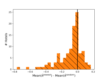
Results.

To validate our theoretical findings, we consider a null hypothesis positing that the probability of $\hat{\pi}^{\textsc{random}}$ having higher mean than $\hat{\pi}^{\textsc{newest}}$ is exactly $50\%$ . In our data, we observe that, for 79 out of 109, the mean of $\hat{\pi}^{\textsc{newest}}$ is strictly smaller than that of $\hat{\pi}^{\textsc{random}}$ which implies a p-value of $5.4\times 10^{-7}$ (and thus rejects the null hypothesis). On average, the mean of $\hat{\pi}^{\textsc{newest}}$ is smaller than that of $\hat{\pi}^{\textsc{random}}$ by $2.3\%$ , or 0.092 points out of 5 in absolute terms. Figure 3 plots a histogram of the difference between these means for the 109 hotels.

Next, in Figure 4, we plot the full distributions of $\hat{\pi}^{\textsc{newest}}$ and $\hat{\pi}^{\textsc{random}}$ for four hotels (in Appendix F, we present the remaining 105 hotels); this is analogous to Figure 2. We observe that $\hat{\pi}^{\textsc{newest}}$ consistently has heavier left tails, while $\hat{\pi}^{\textsc{random}}$ has heavier right tails. This observation matches the theoretical implication of our model (Proposition 3.4).

7 Conclusions

In this paper, we model the idea that customers read only a small number of reviews before making purchase decisions. This model gives rise to the Cost of Newest First, the idea that, when reviews are ordered by newest first, negative reviews will persist as the newest review longer than positive reviews. This phenomenon does not arise in models from the existing literature, since prior works assume that customers incorporate either all reviews or a summary statistic of all reviews into their beliefs. We show that incorporating randomness into the review ordering or using dynamic pricing can alleviate the negative impact of the Cost of Newest First.

Our work opens up a number of intriguing avenues for future research. First, existing literature on social learning studies the self-selection bias (which we do not consider in our model) – how does this self-selection bias interact with the Cost of Newest First? Second, in terms of operational decisions, a platform contains multiple products — should it take the state of reviews into consideration when making display or ranking decisions? Third, given this bounded rationality behavior, are there alternative methods of of disseminating relevant information from reviews? For example, one could succinctly summarize information from all reviews (via, e.g, generative AI) to be the most helpful for each customer. Fourth, we assume that the true quality $\mu$ does not change over time (which enables us to characterize the closed-form expression of the corresponding steady state). Given that changes in the product quality are one of the reasons behind the ubiquitous use of Newest First, it would be interesting to revisit the Cost of Newest First in such dynamic environments. Lastly, on the theoretical side, our analysis fully characterizes the steady state of a stochastic process whose state remains unchanged with some state-dependent probability (Lemma C.3 which is the crux in the analysis of Lemma 3.1). It would be interesting to apply this result to other settings that exhibit a similar structure.

Acknowledgements.

We thank the anonymous reviewers from the 25th ACM Conference on Economics and Computation (EC 2024) for their thorough feedback that greatly improved the presentation of the paper. We are also grateful to the Simons Institute for the Theory of Computing as this work started during the Fall’22 semester-long program on Data Driven Decision Processes.

References

[AGI11] Nikolay Archak, Anindya Ghose, and Panagiotis G Ipeirotis. Deriving the pricing power of product features by mining consumer reviews. Management science, 57(8):1485–1509, 2011.
[AMMO22] Daron Acemoglu, Ali Makhdoumi, Azarakhsh Malekian, and Asuman Ozdaglar. Learning from reviews: The selection effect and the speed of learning. Econometrica, 90(6):2857–2899, 2022.
[Ban92] Abhijit V Banerjee. A simple model of herd behavior. The quarterly journal of economics, 107(3):797–817, 1992.
[BHW92] Sushil Bikhchandani, David Hirshleifer, and Ivo Welch. A theory of fads, fashion, custom, and cultural change as informational cascades. Journal of political Economy, 100(5):992–1026, 1992.
[BMZ12] John W Byers, Michael Mitzenmacher, and Georgios Zervas. The groupon effect on yelp ratings: a root cause analysis. In Proceedings of the 13th ACM conference on electronic commerce, pages 248–265, 2012.
[Bon23] Tommaso Bondi. Alone, together: A model of social (mis)learning from consumer reviews. In Kevin Leyton-Brown, Jason D. Hartline, and Larry Samuelson, editors, Proceedings of the 24th ACM Conference on Economics and Computation, EC 2023, London, United Kingdom, July 9-12, 2023, page 296. ACM, 2023.
[BPS18] Kostas Bimpikis, Yiangos Papanastasiou, and Nicos Savva. Crowdsourcing exploration. Management Science, 64(4):1477–1973, 2018.
[BPS22] Etienne Boursier, Vianney Perchet, and Marco Scarsini. Social learning in non-stationary environments. In International Conference on Algorithmic Learning Theory, pages 128–129. PMLR, 2022.
[BS18] Omar Besbes and Marco Scarsini. On information distortions in online ratings. Operations Research, 66(3):597–610, 2018.
[CDO22] Ishita Chakraborty, Joyee Deb, and Aniko Oery. When do consumers talk? Available at SSRN 4155523, 2022.
[CIMS17] Davide Crapis, Bar Ifrach, Costis Maglaras, and Marco Scarsini. Monopoly pricing in the presence of social learning. Management Science, 63(11):3586–3608, 2017.
[CLT21] Ningyuan Chen, Anran Li, and Kalyan Talluri. Reviews and self-selection bias with operational implications. Management Science, 67(12):7472–7492, 2021.
[CM06] Judith A Chevalier and Dina Mayzlin. The effect of word of mouth on sales: Online book reviews. Journal of marketing research, 43(3):345–354, 2006.
[CSS24] Christoph Carnehl, André Stenzel, and Peter Schmidt. Pricing for the stars: Dynamic pricing in the presence of rating systems. Management Science, 70(3):1755–1772, 2024.
[DLT21] Gregory DeCroix, Xiaoyang Long, and Jordan Tong. How service quality variability hurts revenue when customers learn: Implications for dynamic personalized pricing. Operations Research, 69(3):683–708, 2021.
[FKKK14] Peter Frazier, David Kempe, Jon Kleinberg, and Robert Kleinberg. Incentivizing exploration. In Proceedings of the fifteenth ACM conference on Economics and computation, pages 5–22, 2014.
[Gal97] Robert G Gallager. Discrete stochastic processes. Journal of the Operational Research Society, 48(1):103–103, 1997.
[GHKV23] Wenshuo Guo, Nika Haghtalab, Kirthevasan Kandasamy, and Ellen Vitercik. Leveraging reviews: Learning to price with buyer and seller uncertainty. In Kevin Leyton-Brown, Jason D. Hartline, and Larry Samuelson, editors, Proceedings of the 24th ACM Conference on Economics and Computation, EC 2023, London, United Kingdom, July 9-12, 2023, page 816. ACM, 2023.
[GI10] Anindya Ghose and Panagiotis G Ipeirotis. Estimating the helpfulness and economic impact of product reviews: Mining text and reviewer characteristics. IEEE transactions on knowledge and data engineering, 23(10):1498–1512, 2010.
[GPR06] Jacob K Goeree, Thomas R Palfrey, and Brian W Rogers. Social learning with private and common values. Economic theory, 28:245–264, 2006.
[HC24] Michael Hamilton and Titing Cui. Fresh rating systems: Structure, incentives, and fees. Incentives, and Fees (June 24, 2024), 2024.
[HPZ17] Nan Hu, Paul A Pavlou, and Jie Zhang. On self-selection biases in online product reviews. MIS quarterly, 41(2):449–475, 2017.
[IMSZ19] Bar Ifrach, Costis Maglaras, Marco Scarsini, and Anna Zseleva. Bayesian social learning from consumer reviews. Operations Research, 67(5):1209–1221, 2019.
[Kav21] M Kavanagh. The impact of customer reviews on purchase decisions. Bizrate Insights, available at: https://bizrateinsights.com/resources/the-impact-of-customer-reviews-on-purchase-decisions/ (accessed 4 Feb 2024), 2021.
[KKM⁺17] Sampath Kannan, Michael Kearns, Jamie Morgenstern, Mallesh Pai, Aaron Roth, Rakesh Vohra, and Zhiwei Steven Wu. Fairness incentives for myopic agents. In Proceedings of the 2017 ACM Conference on Economics and Computation, pages 369–386, 2017.
[KMP14] Ilan Kremer, Yishay Mansour, and Motty Perry. Implementing the “wisdom of the crowd”. Journal of Political Economy, 122(5):988–1012, 2014.
[LDRF⁺13] Stephan Ludwig, Ko De Ruyter, Mike Friedman, Elisabeth C Brüggen, Martin Wetzels, and Gerard Pfann. More than words: The influence of affective content and linguistic style matches in online reviews on conversion rates. Journal of marketing, 77(1):87–103, 2013.
[LKAK18] Gaël Le Mens, Balázs Kovács, Judith Avrahami, and Yaakov Kareev. How endogenous crowd formation undermines the wisdom of the crowd in online ratings. Psychological science, 29(9):1475–1490, 2018.
[LLS19] Xiao Liu, Dokyun Lee, and Kannan Srinivasan. Large-scale cross-category analysis of consumer review content on sales conversion leveraging deep learning. Journal of Marketing Research, 56(6):918–943, 2019.
[LS16] Ilan Lobel and Evan Sadler. Preferences, homophily, and social learning. Operations Research, 64(3):564–584, 2016.
[Luc16] Michael Luca. Reviews, reputation, and revenue: The case of yelp. com. Com (March 15, 2016). Harvard Business School NOM Unit Working Paper, (12-016), 2016.
[LYMZ22] Zhanfei Lei, Dezhi Yin, Sabyasachi Mitra, and Han Zhang. Swayed by the reviews: Disentangling the effects of average ratings and individual reviews in online word-of-mouth. Production and Operations Management, 31(6):2393–2411, 2022.
[MSS20] Yishay Mansour, Aleksandrs Slivkins, and Vasilis Syrgkanis. Bayesian incentive-compatible bandit exploration. Operations Research, 68(4):1132–1161, 2020.
[MSSV23] Costis Maglaras, Marco Scarsini, Dongwook Shin, and Stefano Vaccari. Product ranking in the presence of social learning. Operations Research, 71(4):1136–1153, 2023.
[Mur19] Rosie Murphy. Local consumer review survey 2019. Technical report, National Bureau of Economic Research, 2019.
[PSX21] Sungsik Park, Woochoel Shin, and Jinhong Xie. The fateful first consumer review. Marketing Science, 40(3):481–507, 2021.
[RHP23] Hang Ren, Tingliang Huang, and Georgia Perakis. Impact of social learning on consumer subsidies and supplier capacity for green technology adoption. Available at SSRN 4335284, 2023.
[Say18] Amin Sayedi. Pricing in a duopoly with observational learning. Available at SSRN 3131561, 2018.
[SR18] Sven Schmit and Carlos Riquelme. Human interaction with recommendation systems. In International Conference on Artificial Intelligence and Statistics, pages 862–870. PMLR, 2018.
[SS00] Lones Smith and Peter Sørensen. Pathological outcomes of observational learning. Econometrica, 68(2):371–398, 2000.
[ZZ10] Feng Zhu and Xiaoquan Zhang. Impact of online consumer reviews on sales: The moderating role of product and consumer characteristics. Journal of marketing, 74(2):133–148, 2010.

Appendix A Formal definition of the random ordering policy (Section 2.2)

We now show that the policy ${\sigma^{\textsc{random}}}(\mathcal{H}_{t})$ can be defined as the limit of $\sigma^{\textsc{random}(w)}(\mathcal{H}_{t})$ as $w\to\infty$ . For a vector of review ratings $\bm{z}\in\{0,1\}^{c}$ , we denote $N(\bm{z})\coloneqq N_{\bm{z}}=\sum_{i=1}^{c}z_{i}$ . Proposition A.1 implies that as $w\to\infty$ , the draws from $\sigma^{\textsc{random}(w)}$ across different rounds are independent and the distribution $\sigma^{\textsc{random}(w)}(\mathcal{H}_{t})$ approaches the distribution of ${\sigma^{\textsc{random}}}$ .

Proposition A.1.

For any review rating vectors $\bm{z}^{(1)},\bm{z}^{(2)},\ldots,\bm{z}^{(k)}\in\{0,1\}^{c}$ and rounds $t^{(1)}<t^{(2)}<\ldots<t^{(k)}$ , the distribution of reviews by $\sigma^{\textsc{random}(w)}$ approaches the one of $\sigma^{\textsc{random}}$ as $w\to\infty$ , i.e.,

\lim_{w\to\infty}{\mathbb{P}}\Big{[}\forall i\in\{1,\ldots,k\}:\sigma^{\textsc{random}(w)}(\mathcal{H}_{t^{(i)}})=\bm{z}^{(i)}\Big{]}=\prod_{i=1}^{k}{\mathbb{P}}\Big{[}\sigma^{\textsc{random}}(\mathcal{H}_{t^{(i)}})=\bm{z}^{(i)}\Big{]}.

We first show that as $w$ goes to infinity, the $c$ reviews selected by $\sigma^{\textsc{random}(w)}(\mathcal{H}_{t^{(i)}})$ at each round $t^{(i)}$ come from the infinite pool of reviews $\{X_{-i}\}_{i=1}^{\infty}$ with high probability. Let $n_{w}=\lfloor\sqrt{w-t^{(k)}}\rfloor$ be the largest integer such that $n_{w}^{2}\leq w-t^{(k)}$ and let $w$ be large enough so that $n_{w}\geq 1$ . We define $\mathcal{E}^{\textsc{OrderInf}}$ as the event that for every $i\in\{1,\ldots,k\}$ the $c$ reviews selected by $\sigma^{\textsc{random}(w)}(\mathcal{H}_{t^{(i)}})$ come from the set $\{X_{-1},\ldots,X_{-n_{w}^{2}}\}$ . Lemma A.1 shows that $\mathcal{E}^{\textsc{OrderInf}}$ happens with high probability.

Lemma A.1.

${\mathbb{P}}[\mathcal{E}^{\textsc{OrderInf}}]\geq\Big{[}\frac{\binom{n_{w}^{2}}{c}}{\binom{w}{c}}\Big{]}^{k}$ . Furthermore, $\lim_{w\to\infty}{\mathbb{P}}[\mathcal{E}^{\textsc{OrderInf}}]=1$ .

Given that $\sigma^{\textsc{random}(w)}$ selects from the infinite negative pool of reviews with high probability (if $\mathcal{E}^{\textsc{OrderInf}}$ holds), we now derive a concentration bound for the reviews in this pool. Recall that $X_{-\ell}\sim_{i.i.d.}{\mathrm{Bern}}(\mu)$ for $\ell\in\{1,\ldots,n_{w}^{2}\}$ . We partition those reviews into $n_{w}$ groups each containing $n_{w}$ reviews. Let $\mathcal{E}^{\textsc{Conc}}$ be the event that, for each group, the average review rating concentrates around the group’s mean, i.e.

\mathcal{E}^{\textsc{Conc}}=\Big{\{}\forall j\in\{1,\ldots,n_{w}\}:\sum_{\ell=(j-1)\cdot n_{w}+1}^{j\cdot n_{w}}X_{-\ell}\in[\mu(n_{w}-n_{w}^{2/3}),\mu(n_{w}+n_{w}^{2/3})]\Big{\}}.

Our next lemma shows that the concentration event $\mathcal{E}^{\textsc{Conc}}$ happens with high probability.

Lemma A.2.

${\mathbb{P}}\Big{[}\mathcal{E}^{\textsc{Conc}}\Big{]}\geq 1-2n_{w}\exp\Big{(}-\frac{n_{w}^{1/3}\mu}{3}\Big{)}$ . Furthermore, $\lim_{w\to\infty}{\mathbb{P}}\Big{[}\mathcal{E}^{\textsc{Conc}}\Big{]}=1$ .

In order to decompose the left-hand-side of Proposition A.1 into a product of probabilities, we show the following independence lemma.

Lemma A.3.

Let $(y_{1},\ldots,y_{n_{w}^{2}})\in\{0,1\}^{n_{w}^{2}}$ . Then conditioned on $(X_{-1},\ldots,X_{-n_{w}^{2}})=(y_{1},\ldots,y_{n_{w}^{2}})$ and $\mathcal{E}^{\textsc{OrderInf}}$ , the events $\{\sigma^{\textsc{random}}(\mathcal{H}_{t^{(i)}})=\bm{z}^{(i)}\}$ for $i=1,\ldots,k$ are independent.

Having shown independence across rounds, we prove that, for any round $t^{(i)}$ , $\sigma^{\textsc{random}(w)}(\mathcal{H}_{t^{(i)}})$ is close to $\sigma^{\textsc{random}}$ . Let $\mathcal{A}$ be the set of review rating sequences for which event $\mathcal{E}^{\textsc{Conc}}$ holds i.e.

\mathcal{A}=\Big{\{}(y_{1},\ldots,y_{n_{w}^{2}})\in\{0,1\}^{n_{w}^{2}}:\forall j\in\{1,\ldots,n_{w}\},\sum_{\ell=(j-1)\cdot n_{w}+1}^{j\cdot n_{w}}y_{\ell}\in[\mu(n_{w}-n_{w}^{2/3}),\mu(n_{w}+n_{w}^{2/3})]\Big{\}}

Our next lemma shows that if the events $\mathcal{E}^{\textsc{OrderInf}}$ and $\mathcal{E}^{\textsc{Conc}}$ hold, then for any round $t^{(i)}$ , the distribution of $\sigma^{\textsc{random}(w)}(\mathcal{H}_{t^{(i)}})$ is close to the distribution of $\sigma^{\textsc{random}}(\mathcal{H}_{t^{(i)}})$ . To ease notation, we let $X_{-1:n_{w}^{2}}\coloneqq(X_{-1},\ldots,X_{-n_{w}^{2}})$ and $y_{1:n_{w}^{2}}\coloneqq(y_{1},\ldots,y_{n_{w}^{2}})$ .

Lemma A.4.

There exists some function $f:\mathbb{N}\to\mathbb{R}$ satisfying $\lim_{n\to\infty}f(n)=0$ such that assuming that $\mathcal{E}^{\textsc{OrderInf}}$ and $\mathcal{E}^{\textsc{Conc}}$ hold, for any $\bm{z}=(z_{1},\ldots,z_{c})\in\{0,1\}^{c}$ and $(y_{1},\ldots,y_{n_{w}^{2}})\in\mathcal{A}$ :

\Big{|}{\mathbb{P}}\Big{[}\sigma^{\textsc{random}(w)}(\mathcal{H}_{t^{(i)}})=\bm{z}|X_{-1:n_{w}^{2}}=y_{1:n_{w}^{2}}\Big{]}-{\mathbb{P}}\Big{[}\sigma^{\textsc{random}}(\mathcal{H}_{t^{(i)}})=\bm{z}\Big{]}\Big{|}\leq f(n_{w}).

Proof of Proposition A.1.

By Lemma A.1 and Lemma A.2, we can upper bound the probability that neither of $\mathcal{E}^{\textsc{OrderInf}}$ nor $\mathcal{E}^{\textsc{Conc}}$ holds by

{\mathbb{P}}[(\neg\mathcal{E}^{\textsc{OrderInf}})\cup(\neg\mathcal{E}^{\textsc{Conc}})]\leq 1-\Big{[}\frac{\binom{n_{w}^{2}}{c}}{\binom{w}{c}}\Big{]}^{k}+2n_{w}\exp\Big{(}-\frac{n_{w}^{1/3}\mu}{3}\Big{)}\to_{w\to\infty}0.

(5)

We thus assume that $\mathcal{E}^{\textsc{OrderInf}}$ and $\mathcal{E}^{\textsc{Conc}}$ holds which means we focus on sequences $(X_{-1},\ldots,X_{-n_{w}^{2}})\in\mathcal{A}$ . By the law of total probability and the independence of $\sigma^{\textsc{random}(w)}$ across rounds (i.e. Lemma A.3):

		$\displaystyle{\mathbb{P}}\Big{[}\forall i\in\{1,\ldots,k\}:\sigma^{\textsc{random}(w)}(\mathcal{H}_{t^{(i)}})=\bm{z}^{(i)}\|\mathcal{E}^{\textsc{OrderInf}},\mathcal{E}^{\textsc{Conc}}\Big{]}$		(6)
		$\displaystyle=\sum_{(y_{1},\ldots,y_{n_{w}^{2}})\in\mathcal{A}}\underbrace{\prod_{i=1}^{k}{\mathbb{P}}\Big{[}\sigma^{\textsc{random}(w)}(\mathcal{H}_{t^{(i)}})=\bm{z}^{(i)}\|\mathcal{E}^{\textsc{OrderInf}},X_{-1:n_{w}^{2}}=y_{1:n_{w}^{2}}\Big{]}}_{(\textsc{Dec})}\cdot\underbrace{{\mathbb{P}}\big{[}X_{-1:n_{w}^{2}}=y_{1:n_{w}^{2}}\|\mathcal{E}^{\textsc{OrderInf}},\mathcal{E}^{\textsc{Conc}}\big{]}}_{\textsc{Seq}(y_{1:n_{w}^{2}})}.$

By Lemma A.4, we can upper and lower bound this decomposition by

\prod_{i=1}^{k}\Bigg{(}{\mathbb{P}}\Big{[}\sigma^{\textsc{random}}(\mathcal{H}_{t^{(i)}})=\bm{z}^{(i)}\Big{]}-f(n_{w})\Bigg{)}\leq(\textsc{Dec})\leq\prod_{i=1}^{k}\Bigg{(}{\mathbb{P}}\Big{[}\sigma^{\textsc{random}}(\mathcal{H}_{t^{(i)}})=\bm{z}^{(i)}\Big{]}+f(n_{w})\Bigg{)}.

(7)

Recall that $\mathcal{A}$ consists of all sequences $(y_{1},\ldots,y_{n_{w}^{2}})$ that satisfy the event $\mathcal{E}^{\textsc{Conc}}$ . Summing across those sequences and using the independence between the choice of $\sigma^{\textsc{random}(w)}$ (which determines $\mathcal{E}^{\textsc{OrderInf}}$ ) and the values of $X_{-1:n_{w}^{2}}$ (which determine $\mathcal{E}^{\textsc{Conc}}$ ), we obtain

\sum_{(y_{1},\ldots,y_{n_{w}^{2}})\in\mathcal{A}}\textsc{Seq}(y_{1:n_{w}^{2}})={\mathbb{P}}[\mathcal{E}^{\textsc{Conc}}|\mathcal{E}^{\textsc{OrderInf}}]=\underbrace{{\mathbb{P}}[\mathcal{E}^{\textsc{Conc}}]\to_{w\to\infty}1}_{\lx@cref{creftype~refnum}{lemma_bernoulli_concentration_nc}}.

(8)

We conclude the proof by combining (5), (6), (7), (8) and using the fact that $f(n_{w})\to_{w\to\infty}0$ . ∎

A.1 High probability bound on $\mathcal{E}^{\textsc{OrderInf}}$ (Proof of Lemma A.1)

Proof of Lemma A.1.

Fix a particular round $t^{(i)}$ . Note that since $n_{w}=\lfloor\sqrt{w-t^{(k)}}\rfloor$ , the $w$ most recent reviews that $\sigma^{\textsc{random}(w)}(\mathcal{H}_{t^{(i)}})$ considers contain $(X_{-1},\ldots,X_{-n_{w}^{2}})$ . The probability that all $c$ reviews come from that set is $\frac{\binom{n_{w}^{2}}{c}}{\binom{w}{c}}$ . For each round in $t^{(1)},\ldots,t^{(k)}$ , the subset of $c$ reviews is independently drawn by $\sigma^{\textsc{random}(w)}$ . Thus, ${\mathbb{P}}[\mathcal{E}^{\textsc{OrderInf}}]\geq\Big{[}\frac{\binom{n_{w}^{2}}{c}}{\binom{w}{c}}\Big{]}^{k}$ . Next notice that $n_{w}^{2}\geq w-t^{(k)}-1$ and therefore, $\frac{\binom{n_{w}^{2}}{c}}{\binom{w}{c}}\geq\frac{\binom{w-t^{(k)}-1}{c}}{\binom{w}{c}}\to_{w\to\infty}1$ showing the second part. ∎

A.2 Concentration for infinite pool (Proof of Lemma A.2)

Proof of Lemma A.2.

For a fixed $j\in\{1,\ldots,n_{w}\}$ , by Chernoff bound, it holds that

{\mathbb{P}}\Big{[}\sum_{\ell=(j-1)n_{w}+1}^{jn_{w}}X_{-\ell}\in[\mu(n_{w}-n_{w}^{2/3}),\mu(n_{w}+n_{w}^{2/3})]\Big{]}\geq 1-2\exp\Big{(}-\frac{n_{w}^{1/3}\mu}{3}\Big{)}.

By union bound on the $n_{w}$ groups, the event $\mathcal{E}^{\textsc{Conc}}$ has probability at least $1-2n_{w}\exp\Big{(}-\frac{n_{w}^{1/3}\mu}{3}\Big{)}$ . Note that $n_{w}\exp\Big{(}-\frac{n_{w}^{1/3}\mu}{3}\Big{)}\to_{w\to\infty}0$ , which yields the second part. ∎

A.3 Independence of $\sigma^{\textsc{random}(w)}$ across rounds (Proof of Lemma A.3)

Proof of Lemma A.3.

By definition, $\sigma^{\textsc{random}(w)}$ samples a $c$ -sized subset of reviews independently at every round. Thus, conditioning on the subset being sampled from $(X_{-1},\ldots,X_{-n_{w}^{2}})$ , i.e. $\mathcal{E}^{\textsc{OrderInf}}$ , and also conditioning on the exact values of these ratings, i.e. $(X_{-1},\ldots,X_{-n_{w}^{2}})=(y_{1},\ldots,y_{n_{w}^{2}})$ , the draws of $\sigma^{\textsc{random}(w)}(\mathcal{H}_{t^{(i)}})$ are independent for $i=1,\ldots,k$ . ∎

A.4 Single round approximation (Proof of Lemma A.4)

Let $\sigma^{\textsc{random}(w)}(\mathcal{H}_{t^{(i)}})=(Z_{1},\ldots,Z_{c})\in\{0,1\}^{c}$ be the $c$ review ratings chosen from the most recent $w$ reviews. Recall that when $\mathcal{E}^{\textsc{OrderInf}}$ holds, $\sigma^{\textsc{random}(w)}$ selects reviews from $(X_{-1},\ldots,X_{-n_{w}^{2}})$ and that $(X_{-1},\ldots,X_{-n_{w}^{2}})=(y_{1},\ldots,y_{n_{w}^{2}})$ . Let $S_{j}=\{y_{\ell}\}_{\ell=(j-1)\cdot n_{w}+1}^{j\cdot n_{w}}$ for $j\in\{1,\ldots,n_{w}\}$ be a partition of all reviews $(y_{1},\ldots,y_{n_{w}^{2}})$ into $n_{w}$ groups of $n_{w}$ reviews each. We first show that the reviews drawn by $\sigma^{\textsc{random}(w)}(\mathcal{H}_{t^{(i)}})$ come from different groups $S_{j}$ with high probability. Let $\mathcal{E}^{\textsc{diff\_groups}}$ be the event that no two indices $m_{1}<m_{2}\in\{1,\ldots,c\}$ are such that $Z_{m_{1}}$ and $Z_{m_{2}}$ belong to the same group $S_{j}$ for some $j\in\{1,\ldots,n_{w}\}$ . Our next lemma lower bounds the probability of $\mathcal{E}^{\textsc{diff\_groups}}$ .

Lemma A.5.

Assume that $\mathcal{E}^{\textsc{OrderInf}}$ and $\mathcal{E}^{\textsc{Conc}}$ hold. The probability of any two selected indices being of different groups is: ${\mathbb{P}}[\mathcal{E}^{\textsc{diff\_group}}]\geq 1-c!\cdot c^{2}\frac{n_{w}^{2c-1}}{(n_{w}^{2}-c)^{c}}$ and thus $\lim_{w\to\infty}{\mathbb{P}}[\mathcal{E}^{\textsc{diff\_group}}]=1$ .

Proof.

Let $\mathcal{E}_{m_{1},m_{2},j}$ be the event that $Z_{m_{1}},Z_{m_{2}}\in S_{j}$ . Notice that $\mathcal{E}^{\textsc{diff\_group}}$ is exactly the event that none of the $\mathcal{E}_{m_{1},m_{2},j}$ hold. Further, note that $Z_{m_{1}},Z_{m_{2}}\in S_{j}$ implies that $Z_{m_{1}},Z_{m_{1}+1},\ldots,Z_{m_{2}}\in S_{j}$ since we output an ordered set of $c$ reviews by recency. There are thus $\binom{n_{w}}{m_{2}-m_{1}+1}$ ways to choose $Z_{m_{1}},Z_{m_{1}+1},\ldots,Z_{m_{2}}$ to be in the same group $S_{j}$ . Hence the probability of $\mathcal{E}_{m_{1},m_{2},j}$ is at most

{\mathbb{P}}[\mathcal{E}_{m_{1},m_{2},j}]\leq\frac{\binom{n_{w}^{2}}{m_{1}-1}\binom{n_{w}}{m_{2}-m_{1}+1}\binom{n_{w}^{2}}{c-m_{2}}}{\binom{n_{w}^{2}}{c}}

as there are at most $\binom{n_{w}^{2}}{m_{1}-1}$ ways to choose $Z_{1},\ldots,Z_{m_{1}-1}$ and at most $\binom{n_{w}^{2}}{m_{2}-m_{1}}$ ways to choose $Z_{m_{2}+1},\ldots,Z_{c}$ . Using the inequalities $\frac{(n-k)^{k}}{k!}\leq\binom{n}{k}\leq n^{k}$ , we obtain that

{\mathbb{P}}[\mathcal{E}_{m_{1},m_{2},j}]\leq c!\cdot\frac{n_{w}^{2(m_{1}-1)}n_{w}^{m_{2}-m_{1}+1}n_{w}^{2(c-m_{2})}}{(n_{w}^{2}-c)^{c}}=c!\cdot\frac{n_{w}^{2c-(m_{2}-m_{1}+1)}}{(n_{w}^{2}-c)^{c}}\leq c!\cdot\frac{n_{w}^{2c-2}}{(n_{w}^{2}-c)^{c}}

since $m_{2}-m_{1}+1\geq 2$ . Thus, via union bound over $m_{1},m_{2}\in\{1,\ldots,c\}$ and $j\in\{1,\ldots,n_{w}\}$ , i.e., $c^{2}n_{w}$ events, the probability of $\mathcal{E}^{\textsc{diff\_group}}$ is lower bounded as follows

{\mathbb{P}}[\mathcal{E}^{\textsc{diff\_group}}]\geq 1-c^{2}n_{w}\cdot c!\cdot\frac{n_{w}^{2c-2}}{(n_{w}^{2}-c)^{c}}=1-c!\cdot c^{2}\frac{n_{w}^{2c-1}}{(n_{w}^{2}-c)^{c}}\to_{n_{w}\to\infty}1.

∎

When the event $\mathcal{E}^{\textsc{diff\_groups}}$ holds then the reviews $Z_{m}$ for $m=1,\ldots,c$ come from different groups $\{S_{j}\}_{j=1}^{n_{w}}$ . We show that when this happens the values of the reviews $Z_{m}$ are independent. Let $\mathcal{E}_{j_{1},\ldots,j_{c}}$ be the event that review $Z_{m}$ comes from group $S_{j_{m}}$ for $m=1,\ldots,c$ . The next lemma shows that conditioned on the event $\mathcal{E}_{j_{1},\ldots,j_{c}}$ , the values of $Z_{1},\ldots,Z_{c}$ are independent.¹⁶¹⁶16This is not the case without conditioning on $\mathcal{E}_{j_{1},\ldots,j_{c}}$ . As an example, consider two ordered reviews $(Z_{1},Z_{2})$ drawn uniformly from the three ordered review ratings $(1,0,1,1)$ . Conditioned on $Z_{1}=0$ then $Z_{2}=1$ deterministically while conditioned on $Z_{1}=1$ then ${\mathbb{P}}[Z_{2}=0|Z_{1}=1]=\frac{1}{4}$ . As a results $Z_{1}$ and $Z_{2}$ are correlated. Recall that $\mathcal{E}^{\textsc{Conc}}$ implies that $(y_{1},\ldots,y_{n_{w}^{2}})\in\mathcal{A}$ .

Lemma A.6.

Let $j_{1},j_{2}\ldots,j_{c}\in\{1,\ldots,n_{w}\}$ be group indices with $j_{1}<j_{2}<\ldots,\leq j_{c}$ . Conditioned on $\mathcal{E}_{j_{1},\ldots,j_{c}},\mathcal{E}^{\textsc{Conc}}$ , $\mathcal{E}^{\textsc{OrderInf}}$ , and $(y_{1},\ldots,y_{n_{w}^{2}})\in\mathcal{A}$ , for any vector of review ratings $\bm{z}\in\{0,1\}^{c}$ , the events $\{Z_{m}=z_{m}\}$ for $m=1,\ldots,c$ are independent. Furthermore,

{\mathbb{P}}\big{[}Z_{m}=z_{m}\big{]}=\Big{(}\frac{\sum_{\ell\in S_{j_{m}}}y_{\ell}}{n_{w}}\Big{)}^{z_{m}}\Big{(}1-\frac{\sum_{\ell\in S_{j_{m}}}y_{\ell}}{n_{w}}\Big{)}^{1-z_{m}}.

Proof.

For any specific review ratings $y_{\ell_{1}}\in S_{j_{1}},\ldots,y_{\ell_{m}}\in S_{j_{m}}$ , applying Bayes rule

\displaystyle{\mathbb{P}}\big{[}Z_{1}=y_{\ell_{1}},\ldots,Z_{c}=y_{\ell_{c}}|\mathcal{E}_{j_{1},\ldots,j_{c}}\big{]}

\displaystyle=\frac{{\mathbb{P}}\big{[}Z_{1}=y_{\ell_{1}},\ldots,Z_{m}=y_{\ell_{m}},\mathcal{E}_{j_{1},\ldots,j_{c}}\big{]}}{{\mathbb{P}}\big{[}\mathcal{E}_{j_{1},\ldots,j_{c}}\big{]}}

There are $(n_{w})^{c}$ choices for the set of $c$ ratings $(Z_{1},\ldots,Z_{c})$ so that $Z_{m}\in S_{j_{m}}$ for $m=1,\ldots,c$ and $\binom{(n_{w})^{2}}{c}$ total number of choices. Hence $\mathcal{E}_{j_{1},\ldots,j_{c}}$ holds with probability ${\mathbb{P}}\big{[}\mathcal{E}_{j_{1},\ldots,j_{c}}\big{]}=\frac{(n_{w})^{c}}{\binom{(n_{w})^{2}}{c}}$ . Given that there is exactly one choice for the $c$ reviews $(Z_{1},\ldots,Z_{c})$ which satisfies $Z_{1}=y_{\ell_{1}},\ldots,Z_{c}=y_{\ell_{c}}$ :

{\mathbb{P}}\big{[}Z_{1}=y_{\ell_{1}},\ldots,Z_{c}=y_{\ell_{c}}|\mathcal{E}_{\ell_{1},\ldots,\ell_{c}}\big{]}=\frac{\frac{1}{\binom{(n_{w})^{2}}{c}}}{\frac{(n_{w})^{c}}{\binom{(n_{w})^{2}}{c}}}=\frac{1}{(n_{w})^{c}}.

(9)

Since this holds for any $y_{\ell_{1}}\in S_{j_{1}},\ldots,y_{\ell_{m}}\in S_{j_{m}}$ we obtain independence of $\{Z_{m}=z_{m}\}$ for $m=1,\ldots,c$ . By summing (9) over $y_{\ell_{2}},\ldots,y_{\ell_{c}}$ , for any particular $y_{\ell_{m}}\in S_{j_{m}}$ , we have ${\mathbb{P}}[Z_{m}=y_{\ell_{m}}|\mathcal{E}_{\ell_{1},\ldots,\ell_{c}}]=\frac{1}{n_{w}}$ . Therefore, the probability that $Z_{m}$ has a particular value $z_{m}\in\{0,1\}$ is equal to the fraction of $y_{\ell_{m}}\in S_{j_{m}}$ which have value $z_{m}$ i.e.

{\mathbb{P}}\big{[}Z_{m}=z_{m}\big{]}=\Big{(}\frac{\sum_{\ell\in S_{j_{m}}}y_{\ell}}{n_{w}}\Big{)}^{z_{m}}\Big{(}1-\frac{\sum_{\ell\in S_{j_{m}}}y_{\ell}}{n_{w}}\Big{)}^{1-z_{m}}.

∎

We next show that conditioned on the events $\mathcal{E}^{\textsc{diff\_group}}$ , $\mathcal{E}^{\textsc{Conc}}$ , and $\mathcal{E}^{\textsc{OrderInf}}$ the distribution of $\sigma^{\textsc{random}(w)}(\mathcal{H}_{t^{(i)}})$ is close to the distribution of $\sigma^{\textsc{random}}$ . Given that the latter consists of i.i.d. ${\mathrm{Bern}}(\mu)$ , ${\mathbb{P}}(\sigma^{\textsc{random}}=\bm{z})=\mu^{N(\bm{z})}(1-\mu)^{c-N(\bm{z})}$ for vector of review ratings $\bm{z}\in\{0,1\}^{c}$ . Recall that $N(\bm{z})\coloneqq N_{\bm{z}}=\sum_{i=1}^{c}z_{i}$ . Using the independence acorss different groups (Lemma A.6), the following lemma shows that ${\mathbb{P}}[\sigma^{\textsc{random}(w)}(\mathcal{H}_{t^{(i)}})=\bm{z}]$ has a similar decomposition as ${\mathbb{P}}[\sigma^{\textsc{random}}=\bm{z}]$ .

Lemma A.7.

Conditioned on $\mathcal{E}_{j_{1},\ldots,j_{c}},\mathcal{E}^{\textsc{Conc}}$ , $\mathcal{E}^{\textsc{OrderInf}}$ , and $(y_{1},\ldots,y_{n_{w}})\in\mathcal{A}$ , for any vector of review ratings $\bm{z}\in\{0,1\}^{c}$ , ${\mathbb{P}}[\sigma^{\textsc{random}(w)}(\mathcal{H}_{t^{(i)}})=\bm{z}]$ is lower bounded by $(\mu(1-n_{w}^{-\frac{1}{3}}))^{N(\bm{z})}(1-\mu(1+n_{w}^{-\frac{1}{3}}))^{c-N(\bm{z})}$ and upper bounded by $(\mu(1+n_{w}^{-\frac{1}{3}}))^{N(\bm{z})}(1-\mu(1-n_{w}^{-\frac{1}{3}}))^{c-N(\bm{z})}$

Proof.

Using Lemma A.6:

{\mathbb{P}}[\sigma^{\textsc{random}(w)}(\mathcal{H}_{t^{(i)}})=\bm{z}|\mathcal{E}_{j_{1},\ldots,j_{c}}]=\prod_{m=1}^{c}(\frac{\sum_{\ell\in S_{j_{m}}}y_{\ell}}{n_{w}})^{z_{m}}(1-\frac{\sum_{\ell\in S_{j_{m}}}y_{\ell}}{n_{w}})^{1-z_{m}}.

As $(y_{1},\ldots,y_{n_{w}^{2}})\in\mathcal{A}$ , we have that $\mu(1-n_{w}^{-\frac{1}{3}})\leq\frac{\sum_{\ell\in S_{j_{m}}}y_{\ell}}{n_{w}}\leq\mu(1+n_{w}^{-\frac{1}{3}})$ for all $m=1,\ldots,c$ . Applying these inequalities for each $m$ yeilds

	$\displaystyle{\mathbb{P}}[\sigma^{\textsc{random}(w)}(\mathcal{H}_{t^{(i)}})=\bm{z}\|\mathcal{E}_{j_{1},\ldots,j_{c}}]$
	$\displaystyle\in\Big{[}(\mu(1-n_{w}^{-\frac{1}{3}}))^{N(\bm{z})}(1-\mu(1+n_{w}^{-\frac{1}{3}}))^{c-N(\bm{z})},(\mu(1+n_{w}^{-\frac{1}{3}}))^{N(\bm{z})}(1-\mu(1-n_{w}^{-\frac{1}{3}}))^{c-N(\bm{z})}\Big{]}.$

for any $\mathcal{E}_{j_{1},\ldots,j_{c}}$ . As $\mathcal{E}_{\textsc{diff\_groups}}$ is the union of events $\mathcal{E}_{j_{1},\ldots,j_{c}}$ for all indices $j_{1},\ldots,j_{c}$ , this implies

	$\displaystyle{\mathbb{P}}[\sigma^{\textsc{random}(w)}(\mathcal{H}_{t^{(i)}})=\bm{z}\|\mathcal{E}_{\textsc{diff\_groups}}]$
	$\displaystyle\in\Big{[}(\mu(1-n_{w}^{-\frac{1}{3}}))^{N(\bm{z})}(1-\mu(1+n_{w}^{-\frac{1}{3}}))^{c-N(\bm{z})},(\mu(1+n_{w}^{-\frac{1}{3}}))^{N(\bm{z})}(1-\mu(1-n_{w}^{-\frac{1}{3}}))^{c-N(\bm{z})}\Big{]}.$

∎

Proof of Lemma A.4.

The law of total probability yields the following decomposition

	$\displaystyle{\mathbb{P}}[(Z_{1},\ldots,Z_{c})=\bm{z}]$	$\displaystyle={\mathbb{P}}[(Z_{1},\ldots,Z_{c})=\bm{z}\|\mathcal{E}^{\textsc{diff\_group}}]{\mathbb{P}}[\mathcal{E}^{\textsc{diff\_group}}]$
		$\displaystyle+{\mathbb{P}}[(Z_{1},\ldots,Z_{c})=\bm{z}\|\neg\mathcal{E}^{\textsc{diff\_group}}]{\mathbb{P}}[\neg\mathcal{E}^{\textsc{diff\_group}}].$

By this decomposition and Lemma A.7, we can lower bound ${\mathbb{P}}[(Z_{1},\ldots,Z_{c})=\bm{z}]$ by

\displaystyle{\mathbb{P}}[(Z_{1},\ldots,Z_{c})=\bm{z}|\mathcal{E}^{\textsc{diff\_group}}]{\mathbb{P}}[\mathcal{E}^{\textsc{diff\_group}}]\geq\underbrace{(\mu(1-n_{w}^{-\frac{1}{3}}))^{N(\bm{z})}(1-\mu(1+n_{w}^{-\frac{1}{3}}))^{c-N(\bm{z})}{\mathbb{P}}[\mathcal{E}^{\textsc{diff\_group}}]}_{\textsc{LB}(n_{w},\bm{z})}

and upper bound the same probability by

	$\displaystyle{\mathbb{P}}[(Z_{1},\ldots,Z_{c})=\bm{z}\|\mathcal{E}^{\textsc{diff\_group}}]$	$\displaystyle+1-{\mathbb{P}}[\mathcal{E}^{\textsc{diff\_group}}]$
		$\displaystyle\leq\underbrace{(\mu(1+n_{w}^{-\frac{1}{3}}))^{N(\bm{z})}(1-\mu(1-n_{w}^{-\frac{1}{3}}))^{c-N(\bm{z})}+1-{\mathbb{P}}[\mathcal{E}^{\textsc{diff\_group}}]}_{\textsc{UB}(n_{w},\bm{z})}$

Therefore,

\displaystyle|{\mathbb{P}}[(Z_{1},\ldots,Z_{c})=\bm{z}]-\mu^{N(\bm{z})}(1-\mu)^{c-N(\bm{z})}|\leq f(\bm{z},n_{w})

where

\displaystyle f(\bm{z},n_{w})=\max\Big{(}|\textsc{LB}(n_{w},\bm{z})-\mu^{N(\bm{z})}(1-\mu)^{c-N(\bm{z})}|,|\textsc{UB}(n_{w},\bm{z})-\mu^{N(\bm{z})}(1-\mu)^{c-N(\bm{z})}|\Big{)}.

Recall that ${\mathbb{P}}[\sigma^{\textsc{random}}=\bm{z}]=\mu^{N(\bm{z})}(1-\mu)^{c-N(\bm{z})}$ . Since ${\mathbb{P}}[\mathcal{E}^{\textsc{diff\_group}}]\to_{n_{w}\to\infty}1$ (Lemma A.5) and $n_{w}^{-\frac{1}{3}}\to 0$ , we obtain that $f(\bm{z},n_{w})\to_{n\to\infty}0$ for any $\bm{z}\in\{0,1\}^{c}$ because

\textsc{UB}(n_{w},\bm{z}),\textsc{LB}(n_{w},\bm{z})\to_{n_{w}\to\infty}\mu^{N(\bm{z})}(1-\mu)^{c-N(\bm{z})}.

As a result, $f(n_{w})=\max_{\bm{z}\in\{0,1\}^{c}}f(\bm{z},n_{w})$ satisfies the desired property and concludes the proof. ∎

Appendix B Generalizing beyond Beta-Bernoulli distributions (Remark 2.1)

We consider a generalization of the customer behavior model in Section 2. We only point to the modeling assumptions that change; everything else remains as in Section 2:

1.

With respect to the customer valuation, the product’s unobservable part $\mu_{t}$ is drawn from an arbitrary distribution $\mathcal{D}$ with mean $\mu$ and finite support $R=\{r_{1},\ldots,r_{s}\}\in\mathbb{R}^{s}$ where $r_{1}<\ldots<r_{s}$ and $s\geq 2$ . That is, $\mathcal{D}$ is no longer restricted to be Bernoulli with $S=\{0,1\}$ and $\mu$ in $(0,1)$ . This can capture a system where $\mu_{t}$ is the number of stars ( $S=\{1,\ldots,5\}$ ) which is common in online platforms such as Tripadvisor, Airbnb, and Amazon.
2.

With respect to the customer purchase behavior, when presented with a vector of $c$ reviews $\bm{Z}_{t}=(Z_{t,1},\ldots,Z_{t,c})\in S^{c}$ , the customer maps them to an estimated valuation $\hat{V}_{t}=\Theta_{t}+\hat{h}(\bm{Z}_{t})$ , where $\hat{h}:S^{c}\to\mathbb{R}$ is an arbitrary fixed mapping. The model of Section 2.1 is a special case where the estimate $\hat{h}$ is created via a two-stage process: the customer initially creates a posterior belief $\Phi_{t}=\mathrm{Beta}\big{(}a+\sum_{i=1}^{c}Z_{t,i},b+c-\sum_{i=1}^{c}Z_{t,i}\big{)}$ and maps this posterior to an estimate $\hat{h}(\bm{Z}_{t})=h(\Phi_{t})$ via a mapping $h$ . Unlike this special case (where the estimate can only depend on the number of positive reviews in the $c$ displayed reviews), our generalization here allows an arbitrary mapping from $\bm{Z}_{t}$ that can also take the order of reviews into consideration.
3.

With respect to the customer review generation, the review $X_{t}=\mu_{t}$ in the event of a purchase and $X_{t}=\perp$ otherwise. The difference to Section 2 is that $\mu_{t}$ is not restricted to be Bernoulli.
4.

We assume that the estimator $\hat{h}(\bm{z})$ is strictly increasing in each coordinate of the review ratings $\bm{z}$ . This extends Assumption 2.1 in a way that can capture the order of the reviews.
5.

We assume that the customer’s smallest estimated valuation $\underline{\hat{V}}=\Theta+\underline{h}$ where $\underline{h}=\hat{h}(r_{1},\ldots,r_{1})$ has nonzero mass on non-negative numbers, i.e, ${\mathbb{P}}_{\Theta\sim\mathcal{F}}[\underline{\hat{V}}\geq 0]>0$ . This extends Assumption 2.2 and ensures that there exist non-negative prices inducing positive purchase probability.

The main driver behind all results in Sections 3 and 4 is the characterization of the stationary distribution of the Markov chain $\bm{Z}_{t}=(Z_{t,1},\ldots,Z_{t,c})$ of the newest $c$ reviews.

•

Estimator $\hat{h}$ generalizes the customer’s purchase behavior. The purchase probability at a state with review ratings $\bm{z}\in R^{c}$ is ${\mathbb{P}}_{\Theta\sim\mathcal{F}}[\Theta+h(\bm{z})\geq\rho(\bm{z})]$ where $\rho$ is the pricing policy.
•

The review generation process changes the transition dynamics of $\bm{Z}_{t}$ upon a purchase, i.e., a new review takes one of the values $\{r_{1},\ldots,r_{s}\}$ (as opposed to $\{0,1\}$ in the original model).

•

Letting $g_{\mathcal{D}}$ be the probability mass function of $\mathcal{D}$ , the stationary distribution of $\bm{Z}_{t}$ is

\pi_{\bm{z}}=\kappa\cdot\frac{\prod_{i=1}^{c}g_{\mathcal{D}}(r_{i})}{{\mathbb{P}}_{\Theta\sim\mathcal{F}}[\Theta+\hat{h}(\bm{z})\geq\rho(\bm{z})]}\quad\text{where }\kappa=\frac{1}{{\mathbb{E}}_{Z_{1},\ldots,Z_{c}\sim_{i.i.d.}\mathcal{D}}\Big{[}\frac{1}{{\mathbb{P}}_{\Theta\sim\mathcal{F}}[\Theta+\hat{h}(Z_{1},\ldots,Z_{c})\geq\rho(\bm{z})]}\Big{]}}.

•

This is analogous to Lemma 3.1 and Lemma D.5 for static and dynamic pricing in the the Beta-Bernoulli model. In particular, Lemma D.5 replaces $g_{\mathcal{D}}(r_{i})$ and $\hat{h}(\bm{z})$ by $\mu^{z_{i}}(1-\mu)^{1-z_{i}}$ and $h(N_{\bm{z}})$ in the expression for $\pi$ , and the expectation ${\mathbb{E}}_{Z_{1},\ldots,Z_{c}\sim_{i.i.d.}\mathcal{D}}$ and $\hat{h}(Z_{1},\ldots,Z_{c})$ with ${\mathbb{E}}_{Y_{1},\ldots,Y_{c}\sim{\mathrm{Bern}}(\mu)}$ and $h(\sum_{i=1}^{c}Y_{i})$ in the expression for $\kappa$ . The proof is completely analogous.

Using this stationary distribution and similar steps as in the proofs of Proposition 3.3 and Proposition 4.2 the revenue of ${\sigma^{\textsc{newest}}}$ in the generalized model becomes:

\textsc{Rev}(\sigma^{\textsc{newest}},\rho)=\frac{{\mathbb{E}}_{Z_{1},\ldots,z_{c}\sim_{i.i.d.}\mathcal{D}}[\rho(\bm{Z})]}{{\mathbb{E}}_{Z_{1},\ldots,Z_{c}\sim_{i.i.d.}\mathcal{D}}\Big{[}\frac{1}{{\mathbb{P}}_{\Theta\sim\mathcal{F}}[\Theta+\hat{h}(\bm{Z})\geq\rho(\bm{Z})]}\Big{]}}.

The revenue of ${\sigma^{\textsc{random}}}$ (which shows $c$ i.i.d. reviews from $\mathcal{D}$ ) directly follows by adapting the purchase probability in Proposition 3.2 and Theorem 4.3:

{\textsc{Rev}}({\sigma^{\textsc{random}}},\rho)={\mathbb{E}}_{Z_{1},\ldots,Z_{c}\sim_{i.i.d.}\mathcal{D}}\Big{[}\rho(\bm{Z})\cdot{\mathbb{P}}_{\Theta\sim\mathcal{F}}[\Theta+\hat{h}(Z_{1},\ldots,Z_{c})\geq\rho(\bm{Z})]\Big{]}.

Theorem 3.1 and 4.2 then extend to our generalized model by analogously adapting their proofs. With respect to the negative results (Theorem 3.2 and Theorem 4.1), given that the model in the main body is a special case of the generalized model, they also directly extend. With respect to Section 5, similar extensions can be derived under appropriate assumptions; given that those results are about a specific time-discounting model, we do not focus on this extension.

Remark B.1.

The generalized model allows for customers who are fully Bayesian in estimating the fixed valuation given the ordering policy $\sigma$ and use an estimator mapping $\hat{h}=\hat{h}_{\textsc{FullyBayesian}}$ . Such customers could be reactive to $\sigma$ and account for the effect of CoNF; the extension of the CoNF result may thus seem surprising. The reason why this occurs is that CoNF evaluates the customers assuming that they follow the same behavioral model under ${\sigma^{\textsc{random}}}$ and under ${\sigma^{\textsc{newest}}}$ (and does not consider the setting where customers are reactive to the ordering policy).

Appendix C Supplementary material for Section 3

C.1 Absorbing prices cause newest first to get “stuck” (Proposition 3.1)

Proposition 3.1 posits that ${\textsc{Rev}}({\sigma^{\textsc{newest}}},p)=0$ for absorbing prices $p$ . Let $\bm{Z}_{t}=(Z_{t,i})_{i=1}^{c}$ denote the vector of the $c$ most recent reviews at round $t$ . As argued in Section 3.2, $\bm{Z}_{t}$ is a time-homogeneous Markov Chain with a finite state space $\{0,1\}^{c}$ . We say that a state $(z_{1},\ldots,z_{c})\in\{0,1\}^{c}$ of this Markov Chain is absorbing if $\sum_{i=1}^{c}z_{i}\leq n_{0}$ . Given that $p$ is absorbing, an absorbing state will always exist. Once $\bm{Z}_{t}$ enters an absorbing state, no purchase is made thereafter and it stays at the absorbing state forever. Let $\tau(\bm{Z})$ be the first round that $\bm{Z}_{t}$ enters an absorbing state; after this round no purchase is ever made.

To simplify analysis, we define a fictitious Markov chain $\tilde{\bm{Z}_{t}}$ on the same state space that makes transitions with probability $\eta=0$ if ${\mathbb{P}}_{\Theta\sim\mathcal{F}}[\Theta+h(c)\geq p]=0$ and $\eta={\mathbb{P}}_{\Theta\sim\mathcal{F}}[\Theta+h(n_{0})\geq p]$ , where $n_{0}$ is the smallest number of positive reviews that induce a positive purchase probability. If $\tilde{\bm{Z}_{t}}$ is at state $(z_{1},\ldots,z_{c})\in\{0,1\}^{c}$ , then with probability $1-\eta$ , there is no purchase and it remains at the same state. With probability $\eta$ , there is a purchase (and a review); the review is positive with probability $\mu$ (and the state transitions to $(1,z_{1},\ldots,z_{c-1})$ ) and the review is negative with probability $1-\mu$ (and the state transitions to $(0,z_{1},\ldots,z_{c-1})$ ). Notice that $\tilde{\bm{Z}_{t}}$ has the same transitions as $\bm{Z}_{t}$ with the only difference being that the purchase probability is always $\eta$ . Let $\nu(\tilde{\bm{Z}})$ be the first time that $\tilde{\bm{Z}_{t}}$ enters the state $(0,\ldots,0)$ . Our proof relies on the following lemmas.

Lemma C.1.

For $\eta>0$ , $\bm{Z}$ enters an absorbing state before $\tilde{\bm{Z}}$ enters $(0,\ldots,0)$ : ${\mathbb{E}}[\tau(\bm{Z})]\leq{\mathbb{E}}[\nu(\tilde{\bm{Z}})]$ .

Proof.

Consider the following coupling of $\bm{Z}_{t}$ and $\tilde{\bm{Z}}_{t}$ . Let $\{R_{i}\}_{i=1}^{\infty}$ where $R_{i}\sim_{i.i.d.}{\mathrm{Bern}}(\mu)$ be an infinite sequence of i.i.d. ${\mathrm{Bern}}(\mu)$ reviews. We will couple the processes $\bm{Z}_{t}$ and $\tilde{\bm{Z}}_{t}$ by setting $\bm{Z}_{t}=(R_{i_{t}},\ldots,R_{i_{t}+c-1})$ and $\tilde{\bm{Z}_{t}}=(R_{\tilde{i}_{t}},\ldots,R_{\tilde{i}_{t}+c-1})$ where we will update the indices $i_{t}$ and $\tilde{i}_{t}$ as described below. Initially, $i_{1}=\tilde{i}_{1}=1$ . Let $q_{t}={\mathbb{P}}_{\Theta\sim\mathcal{F}}[\Theta+h(\sum_{i=0}^{c-1}R_{i_{t}+i})\geq p]$ be the purchase probability at time $t$ of the process $\bm{Z}_{t}$ . To ensure a purchase occurs in $\tilde{\bm{Z}}_{t}$ only if it also occurs in $\bm{Z}_{t}$ as long as $\bm{Z}_{t}$ is not at an absorbing state, we draw a random number $X_{t}\sim\mathcal{U}[0,1]$ and use the following coupling:

•

Case 1: $X_{t}<\eta$ (both processes get a purchase). $i_{t+1}=i_{t}+1$ and $\tilde{i}_{t+1}=\tilde{i}_{t}+1$ .
•

Case 2: $\eta\leq X_{t}\leq q_{t}$ (only $\bm{Z}_{t}$ gets a purchase). $i_{t+1}=i_{t}+1$ and $\tilde{i}_{t+1}=\tilde{i}_{t}$ .
•

Case 3: $X_{t}>q_{t}$ . $i_{t+1}=i_{t}$ and $\tilde{i}_{t+1}=\tilde{i}_{t}$ .

If $\bm{Z}_{t}$ is at an absorbing state then we only update $\tilde{\bm{Z}}_{t}$ (i.e. $\tilde{i}_{t+1}=\tilde{i}_{t}+1$ with probability $\eta$ and otherwise $\tilde{i}_{t+1}=\tilde{i}_{t}$ ). This coupling ensures that $i_{t}\geq\tilde{i}_{t}$ as long as $\bm{Z}_{t}$ is not at an absorbing state. Since the state $(0,\ldots,0)$ is absorbing, it cannot be the case that $\bm{Z}_{t}$ enters an absorbing state before $\tilde{\bm{Z}}_{t}$ enters $(0,\ldots,0)$ . Thus $\tau(\bm{Z})\leq\nu(\tilde{\bm{Z}})$ which yields the result after taking expectations. ∎

Lemma C.2.

For $\eta>0$ , $\tilde{\bm{Z}}_{t}$ enters $(0,0,\ldots,0)$ after finitely many rounds, i.e., ${\mathbb{E}}[\nu(\tilde{\bm{Z}})]\leq\infty$ .

Proof.

Consider the process $\bm{Y}_{t}=\tilde{\bm{Z}}_{c\cdot t}$ for $t=0,\ldots,$ . For any $\bm{z}\in\{0,1\}^{c}$ , the probability of obtaining $c$ consecutive purchases with negative review is:

{\mathbb{P}}[\bm{Y}_{t+1}=(0,\ldots,0)|\bm{Y}_{t}=\bm{z}]\geq(\eta(1-\mu))^{c}.

(10)

Let $\nu(\bm{Y})=\min\{t\text{ s.t. }\bm{Y}_{t}=(0,\ldots,0)\}$ . By (10), $\nu(\bm{Y})$ is stochastically dominated by a Geometric random variable with success probability $(\eta(1-\mu))^{c}$ , implying ${\mathbb{E}}[\nu(\bm{Y})]\leq\frac{1}{(\eta(1-\mu))^{c}}$ . Since $\bm{Y}_{t}$ only keeps track of every $c$ -th value of $\tilde{\bm{Z}}_{t}$ , $c\cdot\nu(\bm{Y})\geq\nu(\tilde{\bm{Z}})$ and thus ${\mathbb{E}}[\nu(\tilde{\bm{Z}})]\leq c{\mathbb{E}}[\tau(\bm{Y})]\leq\frac{c}{(\eta(1-\mu))^{c}}$ . ∎

Proof of Proposition 3.1.

If ${\mathbb{P}}_{\Theta\sim\mathcal{F}}[\Theta+h(n)\geq p]=0$ for all $n\in\{0,1,\ldots,c\}$ , then no purchase is ever made and ${\textsc{Rev}}({\sigma^{\textsc{newest}}},p)=0$ . We thus focus on the case that there exists some number of positive review ratings $n$ such that ${\mathbb{P}}_{\Theta\sim\mathcal{F}}[\Theta+h(n)\geq p]>0$ . Combining Lemmas C.1 and C.2 yields ${\mathbb{E}}[\tau(\bm{Z})]<\infty$ . For $t>\tau(\bm{Z})$ , $\bm{Z}_{t}$ is absorbing and there is no purchase, i.e., $\Theta_{t}+h(\Phi_{t})\geq\rho(\bm{Z}_{t})$ . Hence, ${\mathbb{E}}\Big{[}\frac{\sum_{t=1}^{T}p\mathbbm{1}_{\Theta_{t}+h(\Phi_{t})}}{T}\Big{]}\leq p\frac{{\mathbb{E}}[\tau(\bm{Z})]}{T}\to 0$ as $T\to\infty$ and ${\textsc{Rev}}({\sigma^{\textsc{newest}}},p)=0$ . ∎

C.2 Stationary Distribution under Newest First (Lemma 3.1)

We first state a general property characterizing how the stationary distribution of a Markov chain changes if we modify it so that in every state, the process remains there with some probability.

Lemma C.3.

Let $\mathcal{M}$ be a Markov chain on a finite state space $\mathcal{S}$ ( $|\mathcal{S}|=m$ ) with a transition probability matrix $M\in\mathbb{R}^{m\times m}$ and a stationary distribution $\pi\in\mathbb{R}^{m}$ . For any function $f:\mathcal{S}\to(0,1]$ , we define a new Markov chain $\mathcal{M}_{f}$ on the same state space $\mathcal{S}$ . At state $s\in\mathcal{S}$ , $\mathcal{M}_{f}$ transitions according to the matrix $M$ with probability $f(s)$ and remains in $s$ with probability $1-f(s)$ . Then $\pi_{f}(s)=\kappa\cdot\frac{\pi(s)}{f(s)}$ is a stationary distribution of $\mathcal{M}_{f}$ where $\kappa=1/\sum_{s\in\mathcal{S}}\frac{\pi(s)}{f(s)}$ is a normalizing constant

Proof of Lemma C.3.

For any state $s\in\mathcal{S}$ , the probability of a self-transition under $\mathcal{M}_{f}$ is $M_{f}(s,s)=f(s)M(s,s)+1-f(s)$ since there are two ways to transition from $s$ back to itself: (1) the $f(s)$ transition followed by a transition back to $s$ via $\mathcal{M}$ and (2) the $1-f(s)$ transition that does not alter the current state. For all states $s\neq s^{\prime}$ , $M_{f}(s,s^{\prime})=f(s)M(s,s^{\prime})$ since the only way for $\mathcal{M}_{f}$ to transition from $s$ to $s^{\prime}$ is to take a $f(s)$ transition at $s$ and follow the transitions of $\mathcal{M}$ to get to $s^{\prime}$ .

The distribution $\Big{\{}\pi_{f}(s)=\kappa\cdot\frac{\pi(s)}{f(s)}\Big{\}}_{s\in\mathcal{S}}$ is a probability distribution by the definition of the normalizing constant $\kappa=1/\sum_{s\in\mathcal{S}}\frac{\pi(s)}{f(s)}$ . Using the transitions of $\mathcal{M}_{f}$ , it holds that:

	$\displaystyle\sum_{s^{\prime}\in\mathcal{S}}\pi_{f}(s^{\prime})M_{f}(s^{\prime},s)$	$\displaystyle=\pi_{f}(s)M_{f}(s,s)+\sum_{s^{\prime}\neq s}\pi_{f}(s^{\prime})M_{f}(s^{\prime},s)$
		$\displaystyle=\pi_{f}(s)\cdot\big{(}1-f(s)+f(s)M(s,s)\big{)}+\sum_{s^{\prime}\neq s}\pi_{f}(s^{\prime})\cdot\big{(}f(s^{\prime})M(s^{\prime},s)\big{)}$
		$\displaystyle=\kappa\cdot\frac{\pi(s)}{f(s)}\cdot\big{(}1-f(s)+f(s)M(s,s)\big{)}+\sum_{s^{\prime}\neq s}\kappa\cdot\frac{\pi(s^{\prime})}{f(s^{\prime})}\cdot\big{(}f(s^{\prime})M(s^{\prime},s)\big{)}$
		$\displaystyle=\kappa\cdot\frac{\pi(s)}{f(s)}-\kappa\cdot\pi(s)+\underbrace{\kappa\cdot\pi(s)M(s,s)+\sum_{s^{\prime}\neq s}\kappa\cdot\pi(s^{\prime})M(s^{\prime},s)}_{=\kappa\cdot\pi(s)\text{ (as $\pi$ is stationary for $\mathcal{M}$)}}=\pi_{f}(s).$

Hence, $\pi_{f}$ is a stationary distribution of $M_{f}$ as $\pi_{f}(s)=\sum_{s^{\prime}\in\mathcal{S}}\pi_{f}(s^{\prime})M_{f}(s^{\prime},s)$ for all states $s$ . ∎

Proof of Lemma 3.1 .

We will show that the stationary distribution of the newest $c$ reviews $\bm{Z}_{t}$ is

\pi_{(z_{1},\ldots,z_{c})}=\kappa\cdot\frac{\mu^{\sum_{i=1}^{c}z_{i}}(1-\mu)^{c-\sum_{i=1}^{c}z_{i}}}{{\mathbb{P}}_{\Theta\sim\mathcal{F}}\Big{[}\Theta+h(\sum_{i=1}^{c}z_{i})\geq p\Big{]}}

where $\kappa=1/{\mathbb{E}}_{N\sim{\mathrm{Binom}}(c,\mu)}\big{[}\frac{1}{{\mathbb{P}}_{\Theta\sim\mathcal{F}}[\Theta+h(N)\geq p]}\big{]}$ is the normalizing constant. In the language of Lemma C.3, $\bm{Z}_{t}$ corresponds to $\mathcal{M}_{f}$ , the state space $\mathcal{S}$ to $\{0,1\}^{c}$ , and $f$ is a function that expresses the purchase probability at a given state, i.e., $f(z_{1},\ldots,z_{c})={\mathbb{P}}_{\Theta\sim\mathcal{F}}\Big{[}\Theta+h(\sum_{i=1}^{c}z_{i})\geq p\Big{]}$ . Note that with probability $1-f(z_{1},\ldots,z_{c})$ , $\bm{Z}_{t}$ remains at the same state (as there is no purchase).

To apply Lemma C.3, we need to show that whenever there is purchase, $\bm{Z}_{t}$ transitions according to a Markov chain with stationary distribution $\mu^{\sum_{i=1}^{c}z_{i}}(1-\mu)^{c-\sum_{i=1}^{c}z_{i}}$ . Consider the Markov chain $\mathcal{M}$ which always replaces the $c$ -th last review with a new ${\mathrm{Bern}}(\mu)$ review. This process has stationary distribution equal to the above numerator and $\bm{Z}_{t}$ transitions according to $\mathcal{M}$ upon a purchase, i.e., with probability $f(z_{1},\ldots,z_{c})$ . As a result, by Lemma C.3, $\pi$ is a stationary distribution for $\bm{Z}_{t}$ . As $\bm{Z}_{t}$ is irreducible and aperiodic, this is the unique stationary distribution. ∎

C.3 Closed-form expression for Cost of Newest First (Lemma 3.2)

Proof of Lemma 3.2.

Dividing the expressions given in Propositions 3.2 and 3.3, the price term $p$ cancels out and the CoNF can be expressed as:

	$\displaystyle\chi(p)$	$\displaystyle={\mathbb{E}}_{N\sim{\mathrm{Binom}}(c,\mu)}\big{[}{\mathbb{P}}_{\Theta\sim\mathcal{F}}[\Theta+h(N)\geq p]\big{]}\cdot{\mathbb{E}}_{N\sim{\mathrm{Binom}}(c,\mu)}\Big{[}\frac{1}{{\mathbb{P}}_{\Theta\sim\mathcal{F}}[\Theta+h(N)\geq p]}\Big{]}$
		$\displaystyle=\Big{(}\sum_{i=0}^{c}\mu^{i}(1-\mu)^{c-i}\binom{c}{i}{\mathbb{P}}_{\Theta\sim\mathcal{F}}[\Theta+h(i)\geq p]\Big{)}\cdot\Big{(}\sum_{j=0}^{c}\mu^{j}(1-\mu)^{c-j}\binom{c}{j}\frac{1}{{\mathbb{P}}_{\Theta\sim\mathcal{F}}[\Theta+h(j)\geq p]}\Big{)}$
		$\displaystyle=\sum_{i,j\in\{0,\ldots,c\}}\mu^{i+j}(1-\mu)^{2c-i-j}\binom{c}{i}\binom{c}{j}\frac{{\mathbb{P}}_{\Theta\sim\mathcal{F}}[\Theta+h(i)\geq p]}{{\mathbb{P}}_{\Theta\sim\mathcal{F}}[\Theta+h(j)\geq p]}.$

∎

C.4 Monotonicity of CoNF under monotone hazard rate (Remark 3.1)

Definition C.1.

A continuous distribution $\mathcal{G}$ with probability and cumulative density functions $g$ and $G$ has Monotone Hazard Rate (MHR) if the hazard rate function $\frac{g(u)}{1-G(u)}$ is non-decreasing in $u$ .

To complement Theorem 3.2, we also show a structural result for the behavior of $\chi(p)$ as a function of $p$ when $\mathcal{F}$ has MHR.

Proposition C.1.

Suppose that $\mathcal{F}$ is a continuous distribution with support $[\underline{\theta},\overline{\theta}]$ and has MHR. Then $\chi(p)$ is non-decreasing for $p\in(\underline{\theta}+h(c),\overline{\theta}+h(0))$ .¹⁷¹⁷17The same proof also extends to cases when $\underline{\theta}=-\infty$ and/or $\overline{\theta}=+\infty$ .

Proof.

By Lemma 3.2, the CoNF is given by

	$\displaystyle\chi(p)$	$\displaystyle=\sum_{i,j\in\{0,\ldots,c\}}\mu^{i+j}(1-\mu)^{2c-i-j}\binom{c}{i}\binom{c}{j}\frac{{\mathbb{P}}_{\Theta\sim\mathcal{F}}[\Theta+h(i)\geq p]}{{\mathbb{P}}_{\Theta\sim\mathcal{F}}[\Theta+h(j)\geq p]}$
		$\displaystyle=\sum_{i=0}^{c}\mu^{2i}(1-\mu)^{2(c-i)}\binom{c}{i}^{2}$
		$\displaystyle\quad+\sum_{i<j}\mu^{i+j}(1-\mu)^{2c-i-j}\binom{c}{i}\binom{c}{j}\Bigg{(}\frac{{\mathbb{P}}_{\Theta\sim\mathcal{F}}[\Theta+h(i)\geq p]}{{\mathbb{P}}_{\Theta\sim\mathcal{F}}[\Theta+h(j)\geq p]}+\frac{{\mathbb{P}}_{\Theta\sim\mathcal{F}}[\Theta+h(j)\geq p]}{{\mathbb{P}}_{\Theta\sim\mathcal{F}}[\Theta+h(i)\geq p]}\Bigg{)}.$

Letting $F$ be the cumulative density function of $\mathcal{F}$ and $\overline{F}(u)\coloneqq 1-F(u)$ be the survival function:

\chi(p)=\sum_{i=0}^{c}\mu^{2i}(1-\mu)^{2(c-i)}\binom{c}{i}^{2}+\sum_{i<j}\mu^{i+j}(1-\mu)^{2c-i-j}\binom{c}{i}\binom{c}{j}\Bigg{(}\frac{\overline{F}(p-h(i))}{\overline{F}(p-h(j))}+\frac{\overline{F}(p-h(j))}{\overline{F}(p-h(i))}\Bigg{)}.

We denote the ratio of the purchase probability with $j$ and $i$ positive reviews by $u_{i,j}(p)\coloneqq\frac{\overline{F}(p-h(j))}{\overline{F}(p-h(i))}$ . For $i<j$ , this ratio is $u_{i,j}(p)\geq 1$ because $p-h(i)>p-h(j)$ due to the monotonicity of $h$ (Assumption 2.1). Given that $\mathcal{F}$ is continuous, $\overline{F}(x)$ is differentiable for any $x$ such that $\overline{F}(x)\in(0,1)$ . Furthermore for $p\in(\underline{\theta}+h(c),\overline{\theta}+h(0))$ , $\overline{F}(p-h(i))\in(0,1)$ for all $i\in\{0,1,\ldots,c\}$ , and thus $u_{i,j}(p)$ is differentiable at $p$ .

We now show that $u_{i,j}(p)$ is non-decreasing in $p$ . Letting $f$ be the probability density function of $\mathcal{F}$ and taking the derivative of $u_{i,j}(p)$ with respect to $p$ :

	$\displaystyle\frac{d}{dp}u_{i,j}(p)$	$\displaystyle=\frac{f(p-h(i))\overline{F}(p-h(j))-f(p-h(j))\overline{F}(p-h(i))}{\overline{F}(p-h(j))^{2}}$
		$\displaystyle=\frac{\Big{(}\frac{f(p-h(i))}{\overline{F}(p-h(i))}-\frac{f(p-h(j))}{\overline{F}(p-h(j))}\Big{)}\overline{F}(p-h(j))\overline{F}(p-h(i))}{\overline{F}(p-h(j))^{2}}.$

Observe that $p-h(i)>p-h(j)$ since $i<j$ and the strict monotonicity of $h$ . By the MHR property of $\mathcal{F}$ : $\frac{f(p-h(i))}{\overline{F}(p-h(i))}\geq\frac{f(p-h(j))}{\overline{F}(p-h(j))}$ , implying that $\frac{d}{dp}u_{i,j}(p)\geq 0$ , and thus $u_{i,j}(p)$ is non-decreasing in $p$ .

To finish the proof of the theorem, we rewrite $\chi(p)$ as a function of $\{u_{i,j}(p)\}_{i<j}$ as

\chi(p)=\sum_{i=0}^{c}\mu^{2i}(1-\mu)^{2(c-i)}\binom{c}{i}^{2}+\sum_{i<j}\mu^{i+j}(1-\mu)^{2c-i-j}\binom{c}{i}\binom{c}{j}\Bigg{(}u_{i,j}(p)+\frac{1}{u_{i,j}(p)}\Bigg{)}

Note that the function $u+\frac{1}{u}$ is non-decreasing for $u\geq 1$ . Since $u_{i,j}(p)\geq 1$ is non-decreasing in $p$ , then $u_{i,j}(p)+\frac{1}{u_{i,j}(p)}$ is monotonically increasing in $p$ for every $i<j$ . Thus, $\chi(p)$ is non-decreasing in $p$ . ∎

C.5 Structure of CoNF for $c=1$ and uniform distributions (Remark 3.1)

To study how $\chi(p)$ depends on the price $p$ we consider a set of instances where a single review is shown ( $c=1$ ) and $\mathcal{F}=\mathcal{U}[0,\overline{\theta}]$ be the uniform distribution on $[0,\overline{\theta}]$ . The set of non-degenerate and non-absorbing prices is $(h(0),h(0)+\overline{\theta})$ . First, we provide a closed form expression for the CoNF.

Proposition C.2.

Let $\mathcal{F}=\mathcal{U}[0,\overline{\theta}]$ and $c=1$ . For $p\in(h(0),h(0)+\overline{\theta})$ , the CoNF is given by

\chi(p)=1+\mu(1-\mu)\Big{(}\frac{\overline{\theta}+h(1)-\max(h(1),p)}{\overline{\theta}-p+h(0)}+\frac{\overline{\theta}-p+h(0)}{\overline{\theta}+h(1)-\max(h(1),p)}-2\Big{)}.

Proof.

By Lemma 3.2 when $c=1$ , the CoNF is given by

	$\displaystyle\chi(p)$	$\displaystyle=\mu^{2}+(1-\mu)^{2}+\mu(1-\mu)\Bigg{(}\frac{{\mathbb{P}}_{\Theta\sim\mathcal{F}}[\Theta+h(1)\geq p]}{{\mathbb{P}}_{\Theta\sim\mathcal{F}}[\Theta+h(0)\geq p]}+\frac{{\mathbb{P}}_{\Theta\sim\mathcal{F}}[\Theta+h(0)\geq p]}{{\mathbb{P}}_{\Theta\sim\mathcal{F}}[\Theta+h(1)\geq p]}\Bigg{)}$
		$\displaystyle=1+\mu(1-\mu)\Bigg{(}\frac{{\mathbb{P}}_{\Theta\sim\mathcal{F}}[\Theta+h(1)\geq p]}{{\mathbb{P}}_{\Theta\sim\mathcal{F}}[\Theta+h(0)\geq p]}+\frac{{\mathbb{P}}_{\Theta\sim\mathcal{F}}[\Theta+h(0)\geq p]}{{\mathbb{P}}_{\Theta\sim\mathcal{F}}[\Theta+h(1)\geq p]}-2\Bigg{)}.$		(11)

For $p\in(h(0),h(0)+\overline{\theta})$ the purchase probabilities with zero and one positive reviews are given by

{\mathbb{P}}_{\Theta\sim\mathcal{F}}[\Theta+h(0)\geq p]=\frac{\overline{\theta}-p+h(0)}{\overline{\theta}}\qquad\text{ and }\qquad{\mathbb{P}}_{\Theta\sim\mathcal{F}}[\Theta+h(1)\geq p]=\frac{\overline{\theta}+h(1)-\max(h(1),p)}{\overline{\theta}}.

Plugging in these probabilities in the expression for CoNF (C.5) concludes the proof. ∎

We next quantify how fast the CoNF increases as $p\to h(0)+\overline{\theta}$ : we show that a price of $p_{k}=\overline{\theta}+h(0)-\Theta(\frac{1}{k})$ results in a CoNF of $\Theta(k)$ . In particular, for $k>1$ we define a target price $p_{k}=\overline{\theta}+h(0)-\min(\frac{\overline{\theta}}{k},\frac{h(1)-h(0)}{k-1})$ and show the following corollary.

Corollary C.1.

Let $\mathcal{F}=\mathcal{U}[0,\overline{\theta}]$ and $c=1$ . For $k>1$ and $p>p_{k}$ , the CoNF is lower bounded by

\chi(p)\geq 1+\mu(1-\mu)(k+\frac{1}{k}-2).

Proof.

We first verify that $p=p_{k}$ is a solution to the equation

\frac{\overline{\theta}+h(1)-\max(h(1),p)}{\overline{\theta}-p+h(0)}=k

(12)

which is equivalent to

pk-\max(h(1),p)=(k-1)\overline{\theta}+kh(0)-h(1).

(13)

If $p\leq h(1)$ , the solution of $(\ref{eq:for_p_k})$ is $p=\overline{\theta}+h(0)-\frac{\overline{\theta}}{k}$ and in order for $p\leq h(1)$ to hold we need $\overline{\theta}+h(0)-\frac{\overline{\theta}}{k}\leq h(1)$ which can be rewritten as $\frac{\overline{\theta}}{k}\leq\frac{h(1)-h(0)}{k-1}$ . As a result, $p_{k}=\overline{\theta}+h(0)-\frac{\overline{\theta}}{k}$ and hence $p_{k}$ satisfies (13).

If $p\geq h(1)$ , the solution is $p=\overline{\theta}+h(0)-\frac{h(1)-h(0)}{k-1}$ and in order for $p\geq h(1)$ to hold we need $\overline{\theta}+h(0)-\frac{h(1)-h(0)}{k-1}\geq h(1)$ which can be rewritten as $\frac{\overline{\theta}}{k}\geq\frac{h(1)-h(0)}{k-1}$ . As a result, $p_{k}=\overline{\theta}+h(0)-\frac{h(1)-h(0)}{k-1}$ and hence $p_{k}$ satisfies (13).

As the first fraction in Proposition C.2 corresponds to (12), we obtain that $\chi(p_{k})=1+\mu(1-\mu)(k+\frac{1}{k}-2)$ . Since $\mathcal{F}=\mathcal{U}[0,\overline{\theta}]$ has MHR, $\chi(p)$ is non-decreasing in $p$ (Proposition C.1) which finishes the proof of the corollary. ∎

C.6 Upper bounding CoNF by the effect of reviews on purchase (Remark 3.2)

Recall that $\beta(p)$ quantifies how much the review ratings affect the purchase probability. It is expected that when the review ratings have a small effect on the purchase probability then the CoNF is also small (i.e. small $\beta(p)$ would imply a small $\chi(p)$ ). We formalize this below.

Proposition C.3.

For all non-absorbing prices $p$ , the CoNF is upper bounded by $\chi(p)\leq\beta(p)$ .

Proof.

The monotonicity of $h$ , implies that for all $n\in\{0,1,\ldots,c\}$ :

{\mathbb{P}}_{\Theta\sim\mathcal{F}}[\Theta+h(c)\geq p]\geq{\mathbb{P}}_{\Theta\sim\mathcal{F}}[\Theta+h(n)\geq p]\geq{\mathbb{P}}_{\Theta\sim\mathcal{F}}[\Theta+h(0)\geq p].

Taking expectation over the number of positive reviews $N\sim{\mathrm{Binom}}(c,\mu)$ , the first inequality implies

{\mathbb{E}}_{N\sim{\mathrm{Binom}}(c,\mu)}\big{[}{\mathbb{P}}_{\Theta\sim\mathcal{F}}[\Theta+h(N)\geq p]\big{]}\leq{\mathbb{P}}_{\Theta\sim\mathcal{F}}[\Theta+h(c)\geq p].

(14)

Similarly, taking expectation of the the reciprocal of the second inequality (which is well-defined as $p$ is non-absorbing) implies that

{\mathbb{E}}_{N\sim{\mathrm{Binom}}(c,\mu)}\Big{[}\frac{1}{{\mathbb{P}}_{\Theta\sim\mathcal{F}}[\Theta+h(N)\geq p]}\Big{]}\leq\frac{1}{{\mathbb{P}}_{\Theta\sim\mathcal{F}}[\Theta+h(0)\geq p]}.

(15)

Expressing $\chi(\pi)$ as the ratio of the expressions in Propositions 3.2 and 3.3 and using (14) and (15):

	$\displaystyle\chi(p)$	$\displaystyle={\mathbb{E}}_{N\sim{\mathrm{Binom}}(c,\mu)}[{\mathbb{P}}_{\Theta\sim\mathcal{F}}[\Theta+h(N)\geq p]]\cdot{\mathbb{E}}_{N\sim{\mathrm{Binom}}(c,\mu)}\Big{[}\frac{1}{{\mathbb{P}}_{\Theta\sim\mathcal{F}}[\Theta+h(N)\geq p]}\Big{]}$
		$\displaystyle\leq\frac{{\mathbb{P}}_{\Theta\sim\mathcal{F}}[\Theta+h(c)\geq p]}{{\mathbb{P}}_{\Theta\sim\mathcal{F}}[\Theta+h(0)\geq p]}=\beta(p)$

which concludes the proof. ∎

C.7 Average rating under ${\sigma^{\textsc{newest}}}$ is smaller than under ${\sigma^{\textsc{random}}}$ (Theorem 3.3)

Theorem 3.3 states that the average review rating of the $c$ reviews displayed by ${\sigma^{\textsc{newest}}}$ is strictly smaller than the average rating of the $c$ reviews displayed by ${\sigma^{\textsc{random}}}$ . To prove the theorem we first compare the behavior of ${\sigma^{\textsc{newest}}}$ and ${\sigma^{\textsc{random}}}$ based on $n^{\star}=\max\{n|{\mathbb{P}}_{\Theta\sim\mathcal{F}}[\Theta+h(n)\geq p]\leq\kappa\}$ (i.e., the largest number of positive review ratings where the purchase probability is at most the average purchase rate $\kappa=1/{\mathbb{E}}_{N\sim{\mathrm{Binom}}(c,\mu)}\Big{[}\frac{1}{{\mathbb{P}}_{\Theta\sim\mathcal{F}}[\Theta+h(N)\geq p]}\Big{]}$ ).

Lemma C.4.

For non-degenerate and non-absorbing price $p$ , $\pi^{\textsc{newest}}_{n}\leq\pi^{\textsc{random}}_{n}$ if $n>n^{\star}$ and $\pi^{\textsc{newest}}_{n}\geq\pi^{\textsc{random}}_{n}$ if $n\leq n^{\star}$ .

Proof of Lemma C.4.

By Lemma 3.1, it holds that $\pi^{\textsc{random}}_{n}=\pi^{\textsc{newest}}_{n}\cdot\frac{1}{\kappa}\cdot{\mathbb{P}}_{\Theta\sim\mathcal{F}}[\Theta+h(n)\geq p]$ . By the definition of $n^{\star}$ and the monotonicity of $h(n)$ , if $n\leq n^{\star}$ , ${\mathbb{P}}_{\Theta\sim\mathcal{F}}[\Theta+h(n)\geq p]\leq\kappa$ and thus $\pi^{\textsc{newest}}_{n}\geq\pi^{\textsc{random}}_{n}$ . The other case is analogous. ∎

Lemma C.5.

For any non-degenerate and non-absorbing price $p$ , the probability of showing at most $n^{\star}$ positive review ratings is strictly larger under ${\sigma^{\textsc{newest}}}$ than under ${\sigma^{\textsc{random}}}$ . Formally, ${\mathbb{P}}_{N\sim\pi_{n}^{\textsc{newest}}}[N\leq n^{\star}]>{\mathbb{P}}_{N\sim\pi_{n}^{\textsc{random}}}[N\leq n^{\star}]$ .

Proof of Lemma C.5.

By Lemma C.4, $\pi^{\textsc{newest}}_{n}\geq\pi^{\textsc{random}}_{n}$ for $n\leq n^{\star}$ . To show the claim it is enough to show that there is some $n\leq n^{\star}$ such that $\pi^{\textsc{newest}}_{n}<\pi^{\textsc{random}}_{n}$ . We show that the purchase probability when all reviews are negative is strictly greater under ${\sigma^{\textsc{newest}}}$ than under ${\sigma^{\textsc{random}}}$ i.e. $\pi^{\textsc{newest}}_{0}<\pi^{\textsc{random}}_{0}$ . By the monotonicity of $h$ , ${\mathbb{P}}_{\Theta\sim\mathcal{F}}[\Theta+h(0)\geq p]\leq{\mathbb{P}}_{\Theta\sim\mathcal{F}}[\Theta+h(n)\geq p]$ for all $n\in\{0,1\ldots,c\}$ . Since $p$ is non-degenerate, the inequality is strict when $n=c$ . Taking the reciprocal and expectation of the last inequality yields the result. ∎

Proof of Theorem 3.3.

To show that the average rating is smaller under ${\sigma^{\textsc{newest}}}$ compared to ${\sigma^{\textsc{random}}}$ ,

	$\displaystyle{\mathbb{E}}_{N\sim\pi^{\textsc{random}}_{n}}[N]-{\mathbb{E}}_{N\sim\pi^{\textsc{newest}}_{n}}[N]$	$\displaystyle=\sum_{m=0}^{c}m(\pi^{\textsc{random}}_{m}-\pi^{\textsc{newest}}_{m})$
		$\displaystyle=\underbrace{\sum_{m=n^{\star}+1}^{c}m(\pi^{\textsc{random}}_{m}-\pi^{\textsc{newest}}_{m})}_{(1)}-\underbrace{\sum_{m=0}^{n^{\star}}m(\pi^{\textsc{newest}}_{m}-\pi^{\textsc{random}}_{m})}_{(2)}$

Lemma C.4 yields $(\pi^{\textsc{random}}_{m}-\pi^{\textsc{newest}}_{m})\geq 0$ for $m\geq n^{\star}+1$ and thus

	$\displaystyle(1)$	$\displaystyle\geq(n^{\star}+1)\sum_{m=n^{\star}+1}^{c}(\pi^{\textsc{random}}_{m}-\pi^{\textsc{newest}}_{m})$
		$\displaystyle=(n^{\star}+1)\big{(}{\mathbb{P}}_{N\sim\pi_{n}^{\textsc{random}}}[N>n^{\star}]-{\mathbb{P}}_{N\sim\pi_{n}^{\textsc{newest}}}[N>n^{\star}]\big{)}$
		$\displaystyle=(n^{\star}+1)\big{(}{\mathbb{P}}_{N\sim\pi_{n}^{\textsc{newest}}}[N\leq n^{\star}]-{\mathbb{P}}_{N\sim\pi_{n}^{\textsc{random}}}[N\leq n^{\star}]\big{)}$

where in the last equality we used that ${\mathbb{P}}[X>n^{\star}]=1-{\mathbb{P}}[X\leq n^{\star}]$ for any random variable $X$ . Using Lemma C.4 again yields $(\pi^{\textsc{newest}}_{m}-\pi^{\textsc{random}}_{m})\geq 0$ for $m\leq n^{\star}$ and thus

(2)\leq n^{\star}\sum_{m=0}^{n^{\star}}(\pi^{\textsc{newest}}_{m}-\pi^{\textsc{random}}_{m})=n^{\star}\big{(}{\mathbb{P}}_{N\sim\pi_{n}^{\textsc{newest}}}[N\leq n^{\star}]-{\mathbb{P}}_{N\sim\pi_{n}^{\textsc{random}}}[N\leq n^{\star}]\big{)}.

Therefore by Lemma C.5,

(1)-(2)\geq\big{(}{\mathbb{P}}_{N\sim\pi_{n}^{\textsc{newest}}}[N\leq n^{\star}]-{\mathbb{P}}_{N\sim\pi_{n}^{\textsc{random}}}[N\leq n^{\star}]\big{)}>0.

∎

Appendix D Supplementary material for Section 4

D.1 CoNF still exists under optimal dynamic pricing (Proposition 4.1)

Proof of Proposition 4.1.

For any $\alpha<4/3$ , we provide an instance with $\chi(\Pi^{\textsc{dynamic}})=\alpha$ . The instance consists of a single review $(c=1)$ , true quality $\mu<\frac{1}{3}$ , estimate mappings $h(0)=\mu^{2}$ , $h(1)=1-\mu^{2}$ , and customer-specific valuation $\mathcal{F}=\mathcal{U}[0,2\overline{h}]$ where $\overline{h}\coloneqq{\mathbb{E}}_{N}[h(N)]$ .

First, for any $A>0$ and any price $p$ the revenue of selling to a customer with valuation $V=Y+x$ where $Y\sim\mathcal{U}[0,A]$ is given by $p\cdot{\mathbb{P}}[V\geq p]=\frac{p(A+x-p)}{A}$ if $p\in[x,A+x]$ . Thus, the revenue maximizing price is $p^{\star}=\max(\frac{A+x}{2},x)=\frac{\max(x,A)+x}{2}$ yielding an optimal revenue of

\max_{p}\{p\cdot{\mathbb{P}}[V\geq p]\}=\frac{\max(x,A)+x}{2}\cdot\frac{2A+x-\max(A,x)}{2A}=\frac{(\max(A,x)+x)^{2}}{4\max(A,x)}.

(16)

Theorems 4.3 and 4.5 imply that $\chi(\Pi^{\textsc{dynamic}})=\frac{{\mathbb{E}}_{N}[r^{\star}(\Theta+h(N))]}{r^{\star}(\Theta+\overline{h})}$ . Using (16) with $A=2\overline{h}$ , we obtain

r^{\star}(\Theta+x)=\frac{(\max(2\overline{h},x)+x)^{2}}{4\max(2\overline{h},x)}=\begin{cases}\frac{9}{8}\overline{h}&\text{if }x=\overline{h}\\ h(1)&\text{if }x=h(1)\\ \frac{(h(0)+2\overline{h})^{2}}{8\overline{h}}&\text{if }x=h(0)\end{cases}.

(17)

where $\max(2\overline{h},h(1))=h(1)$ because $2\mu(1-\mu)(1+2\mu)=2\mu(1+\mu-2\mu^{2})<2\mu(1+\mu)<\frac{8}{9}<1-\mu^{2}$ for $\mu<\frac{1}{3}$ and thus

2\overline{h}=2(\mu h(1)+(1-\mu)h(0))=2\big{(}\mu(1-\mu^{2})+(1-\mu)\mu^{2}\big{)}=2\mu(1-\mu)(1+2\mu)<1-\mu^{2}=h(1).

Using (17) , the CoNF can be expressed as:

	$\displaystyle\chi(\Pi^{\textsc{dynamic}})$	$\displaystyle=\frac{{\mathbb{E}}_{N}[r^{\star}(\Theta+h(N))]}{r^{\star}(\Theta+\overline{h})}=\frac{\mu r^{\star}(\Theta+h(1))+(1-\mu)r^{\star}(\Theta+h(0))}{r^{\star}(\Theta+\overline{h})}$
		$\displaystyle\overset{(1)}{=}\frac{\mu h(1)+(1-\mu)\frac{(h(0)+2\overline{h})^{2}}{8\overline{h}}}{\frac{9}{8}\overline{h}}=\frac{8}{9}\cdot\frac{\mu h(1)}{\overline{h}}+\frac{1-\mu}{9}\Big{[}\Big{(}\frac{h(0)}{\overline{h}}\Big{)}^{2}+4\frac{h(0)}{\overline{h}}+4\Big{]}$
		$\displaystyle\overset{(2)}{=}\frac{8}{9}-\frac{8}{9}\cdot\frac{(1-\mu)h(0)}{\overline{h}}+\frac{1-\mu}{9}\cdot\Big{(}\frac{h(0)}{\overline{h}}\Big{)}^{2}+\frac{1-\mu}{9}\cdot 4\frac{h(0)}{\overline{h}}+\frac{1-\mu}{9}\cdot 4$
		$\displaystyle\overset{(3)}{=}\frac{8}{9}+\frac{1-\mu}{9}\Big{[}\Big{(}\frac{h(0)}{\overline{h}}\Big{)}^{2}-4\frac{h(0)}{\overline{h}}+4\Big{]}=\frac{8}{9}+\frac{1-\mu}{9}\Big{(}\frac{h(0)}{\overline{h}}-2\Big{)}^{2}$
		$\displaystyle\overset{(4)}{=}\frac{8}{9}+\frac{1-\mu}{9}(\frac{\mu}{1+\mu-2\mu^{2}}-2)^{2}$

where (1) follows by the expression for the optimal revenue (17), (2) follows by $\frac{\mu h(1)}{\overline{h}}=1-\frac{(1-\mu)h(0)}{\overline{h}}$ which follows by the definition of $\overline{h}$ , (3) follows by $-\frac{8}{9}\cdot\frac{(1-\mu)h(0)}{\overline{h}}+\frac{1-\mu}{9}\cdot 4\frac{h(0)}{\overline{h}}=-\frac{1-\mu}{9}\cdot 4\frac{h(0)}{\overline{h}}$ , and (4) follows by $\frac{h(0)}{\overline{h}}=\frac{\mu^{2}}{\mu(1-\mu)(1+2\mu)}=\frac{\mu}{1+\mu-2\mu^{2}}$ because $h(0)=\mu^{2}$ and $\overline{h}=\mu(1-\mu)(1+2\mu)$ .

Thus, $\chi(\Pi^{\textsc{dynamic}})=\frac{8}{9}+\frac{1-\mu}{9}(\frac{\mu}{1+\mu-2\mu^{2}}-2)^{2}$ . The second term is $\frac{1-\mu}{9}(\frac{\mu}{1+\mu-2\mu^{2}}-2)^{2}\to\frac{4}{9}$ as $\mu\to 0$ , and thus $\chi(\Pi^{\textsc{dynamic}})\to\frac{8}{9}+\frac{4}{9}=\frac{4}{3}$ as $\mu\to 0$ . Therefore, for any $\alpha<4/3$ there is some sufficiently small $\mu>0$ such that $\chi(\Pi^{\textsc{dynamic}})>\alpha$ . ∎

D.2 $\sigma^{\textsc{random}}$ is no worse than $\sigma^{\textsc{newest}}$ under optimal dynamic pricing (Remark 4.1)

Theorem 3.1 established that $\chi(p)>1$ for any fixed non-degenerate and non-absorbing price $p$ . Here we show that if the platform optimizes over dynamic prices we have $\chi(\Pi^{\textsc{dynamic}})\geq 1$ i.e. ${\sigma^{\textsc{random}}}$ has no smaller revenue that ${\sigma^{\textsc{newest}}}$ under optimal dynamic prices. Recall that $\chi(\Pi^{\textsc{dynamic}})=\frac{\max_{\rho\in\Pi^{\textsc{dynamic}}}\textsc{Rev}(\sigma^{\textsc{random}},\rho)}{\max_{\rho\in\Pi^{\textsc{dynamic}}}\textsc{Rev}(\sigma^{\textsc{newest}},\rho)}$ . We show the following result.

Theorem D.1.

For any problem instance, $\chi(\Pi^{\textsc{dynamic}})\geq 1$ .

Proof.

By definition of $\chi(\Pi^{\textsc{dynamic}})$ , it is sufficient to show that

\max_{\rho\in\Pi^{\textsc{dynamic}}}\textsc{Rev}(\sigma^{\textsc{newest}},\rho)\leq\max_{\rho\in\Pi^{\textsc{dynamic}}}\textsc{Rev}(\sigma^{\textsc{random}},\rho).

(18)

Letting $\overline{h}={\mathbb{E}}_{N\sim{\mathrm{Binom}}(c,\mu)}[h(N)]$ and $p^{\star}\in\operatorname*{arg\,max}_{p\in\mathbb{R}}p{\mathbb{P}}_{\Theta\sim\mathcal{F}}[\Theta+\overline{h}\geq p]$ , Theorem 4.4 yields that the pricing policy given by $\rho^{\textsc{newest}}(\bm{z})=h(N_{\bm{z}})+p^{\star}-\overline{h}$ is optimal under $\sigma^{\textsc{newest}}$ and is thus the maximizer of the left-hand side of (18). To prove (18) it is sufficient to show that offering prices $\rho^{\textsc{newest}}(\bm{z})$ under $\sigma^{\textsc{random}}$ yields the same revenue as offering prices $\rho^{\textsc{newest}}(\bm{z})$ under $\sigma^{\textsc{newest}}$ i.e. $\textsc{Rev}(\sigma^{\textsc{random}},\rho^{\textsc{newest}})=\textsc{Rev}(\sigma^{\textsc{newest}},\rho^{\textsc{newest}})$ .

As $\sigma^{\textsc{random}}$ shows $c$ i.i.d. ${\mathrm{Bern}}(\mu)$ reviews, the revenue of any pricing policy $\rho$ is given by

{\textsc{Rev}}({\sigma^{\textsc{random}}},\rho)={\mathbb{E}}_{Z_{1},\ldots,Z_{c}\sim_{i.i.d}{\mathrm{Bern}}(\mu)}\Big{[}\rho(Z_{1},\ldots,Z_{c}){\mathbb{P}}_{\Theta\sim\mathcal{F}}[\Theta+h(\sum_{i=1}^{c}Z_{i})\geq\rho(Z_{1},\ldots,Z_{c})]\Big{]}.

(19)

For any reviews $(Z_{1},\ldots,Z_{c})$ the purchase probability under $\rho^{\textsc{newest}}(Z_{1},\ldots,Z_{c})$ equals

{\mathbb{P}}_{\Theta\sim\mathcal{F}}\Big{[}\Theta+h(\sum_{i=1}^{c}Z_{i})\geq h(\sum_{i=1}^{c}Z_{i})+p^{\star}-\overline{h}\Big{]}={\mathbb{P}}_{\Theta\sim\mathcal{F}}[\Theta+\overline{h}\geq p^{\star}]

(20)

and is independent of $(Z_{1},\ldots,Z_{c})$ . As $Z_{1},\ldots,Z_{c}\sim_{i.i.d.}{\mathrm{Bern}}(\mu)$ , the number of positive review ratings $\sum_{i=1}^{c}Z_{i}$ is distributed as $N\sim{\mathrm{Binom}}(c,\mu)$ ; the expected price of $\rho^{\textsc{newest}}(Z_{1},\ldots,Z_{c})$ is thus

{\mathbb{E}}_{Z_{1},\ldots,Z_{c}\sim_{i.i.d}{\mathrm{Bern}}(\mu)}\Big{[}\rho^{\textsc{newest}}(Z_{1},\ldots,Z_{c})\Big{]}={\mathbb{E}}_{N\sim{\mathrm{Binom}}(c,\mu)}[h(N)+p^{\star}-\overline{h}]=p^{\star}

(21)

where the last equality uses the definition of $\overline{h}={\mathbb{E}}_{N\sim{\mathrm{Binom}}(c,\mu)}[h(N)]$ . Combining (19), (20),and (21), we obtain ${\textsc{Rev}}({\sigma^{\textsc{random}}},\rho)=p^{\star}{\mathbb{P}}_{\Theta\sim\mathcal{F}}[\Theta+\overline{h}\geq p^{\star}]=r^{\star}(\Theta+\overline{h})$ . The last expression is exactly equal to $\max_{\rho\in\Pi^{\textsc{dynamic}}}\textsc{Rev}(\sigma^{\textsc{newest}},\rho)$ by Theorem 4.5 which concludes the proof. ∎

Another way to prove Theorem D.1 stems from using the convexity of $r^{\star}(\Theta+x)$ , defined in the beginning of Section 4.2. This is shown in the lemma below.

Lemma D.1.

$r^{\star}(\Theta+x)$ is a convex function in $x$ .

Alternative proof of Theorem D.1.

By Theorem 4.3 and Theorem 4.5, we know that

\max_{\rho\in\Pi^{\textsc{dynamic}}}\textsc{Rev}(\sigma^{\textsc{random}},\rho)={\mathbb{E}}_{N\sim{\mathrm{Binom}}(c,\mu)}[r^{\star}(\Theta+h(N))]

and

\max_{\rho\in\Pi^{\textsc{dynamic}}}\textsc{Rev}(\sigma^{\textsc{newest}},\rho)=r^{\star}(\Theta+{\mathbb{E}}_{N\sim{\mathrm{Binom}}(c,\mu)}[h(N)]).

By Lemma D.1 $r^{\star}(\Theta+x)$ is convex. Thus by Jensen’s inequality the theorem follows as

r^{\star}(\Theta+{\mathbb{E}}_{N\sim{\mathrm{Binom}}(c,\mu)}[h(N)])\leq{\mathbb{E}}_{N\sim{\mathrm{Binom}}(c,\mu)}[r^{\star}(\Theta+h(N))].

∎

Proof of Lemma D.1.

Let $x,y\in\mathbb{R},\alpha\in[0,1]$ . To show that $r^{\star}(\Theta+x)$ is convex, it suffices to prove that

\max_{p\in\mathbb{R}}p{\mathbb{P}}_{\Theta\sim\mathcal{F}}[\Theta+\alpha x+(1-\alpha)y\geq p]\leq\alpha\max_{p\in\mathbb{R}}p{\mathbb{P}}_{\Theta\sim\mathcal{F}}[\Theta+x\geq p]+(1-\alpha)\max_{p\in\mathbb{R}}p{\mathbb{P}}_{\Theta\sim\mathcal{F}}[\Theta+y\geq p]

Let $p\in\operatorname*{arg\,max}p{\mathbb{P}}_{\Theta\sim\mathcal{F}}[\Theta+\alpha x+(1-\alpha)y\geq p]$ be an optimal price for selling to a customer with valuation $\Theta+\alpha x+(1-\alpha)y$ . We define two prices $p_{1}\coloneqq p-(1-\alpha)(y-x)$ and $p_{2}\coloneqq p-\alpha(x-y)$ . The probability that a customer with valuation $\Theta+x$ purchases under $p_{1}$ equals the probability that a customer with valuation $\Theta+\alpha x+(1-\alpha)y$ purchases under $p$ and thus

p_{1}{\mathbb{P}}_{\Theta\sim\mathcal{F}}[\Theta+x\geq p_{1}]=p_{1}{\mathbb{P}}_{\Theta\sim\mathcal{F}}[\Theta+\alpha x+(1-\alpha)y\geq p].

Similarly, a customer with valuation $\Theta+y$ purchases under $p_{2}$ equals the probability that a customer with valuation $\Theta+\alpha x+(1-\alpha)y$ purchases under $p$ and thus

p_{2}{\mathbb{P}}_{\Theta\sim\mathcal{F}}[\Theta+x\geq p_{2}]=p_{2}{\mathbb{P}}_{\Theta\sim\mathcal{F}}[\Theta+\alpha x+(1-\alpha)y\geq p].

Therefore, rearranging and using that $\alpha p_{1}+(1-\alpha)p_{2}=p$ we obtain

\alpha p_{1}{\mathbb{P}}_{\Theta\sim\mathcal{F}}[\Theta+x\geq p_{1}]+(1-\alpha)p_{2}{\mathbb{P}}_{\Theta\sim\mathcal{F}}[\Theta+x\geq p_{2}]=p{\mathbb{P}}_{\Theta\sim\mathcal{F}}[\Theta+\alpha x+(1-\alpha)y\geq p].

Upper bounding the left-hand side, the proof of the lemma concludes as

\alpha\max_{p_{1}\in\mathbb{R}}p_{1}{\mathbb{P}}_{\Theta\sim\mathcal{F}}[\Theta+x\geq p_{1}]+(1-\alpha)\max_{p_{2}\in\mathbb{R}}p_{2}{\mathbb{P}}_{\Theta\sim\mathcal{F}}[\Theta+y\geq p_{2}]\geq p{\mathbb{P}}_{\Theta\sim\mathcal{F}}[\Theta+\alpha x+(1-\alpha)y\geq p].

∎

D.3 Stronger CoNF upper bound under further assumptions on $h$ (Remark 4.2)

Theorem D.2.

For any instance with $h(n)\leq u$ for all $n\in\{0,1,\ldots,c\}$ : $\chi(\Pi^{\textsc{dynamic}})\leq\frac{2{\mathbb{P}}_{\Theta\sim\mathcal{F}}[\Theta\geq-u]}{{\mathbb{P}}_{\Theta\sim\mathcal{F}}[\Theta\geq 0]}$

Proof.

Similar to the proof of Theorem 4.2, we define $\tilde{p}_{n}=\overline{h}+\max(p^{\star}(\Theta+h(n))-h(n),0)$ and let $p(n)=p^{\star}(\Theta+h(n))$ for convenience. We refine the analysis of Lemma 4.5, to show that for any $n\in\{0,1,\ldots,c\}$ , $\textsc{Demand Ratio}(\tilde{p}_{n},n)\leq\frac{{\mathbb{P}}_{\Theta\sim\mathcal{F}}[\Theta\geq-u]}{{\mathbb{P}}_{\Theta\sim\mathcal{F}}[\Theta\geq 0]}$ . We consider two cases:

•

If $p(n)\geq h(n)$ , then $\max(p(n)-h(n),0)=p(n)-h(n)$ and thus

\textsc{Demand Ratio}(\tilde{p}_{n},n)=\frac{{\mathbb{P}}_{\Theta\sim\mathcal{F}}\big{[}\Theta\geq p(n)-h(n)\big{]}}{{\mathbb{P}}_{\Theta\sim\mathcal{F}}\big{[}\Theta\geq\max(p(n)-h(n),0)\big{]}}=1\leq\frac{{\mathbb{P}}_{\Theta\sim\mathcal{F}}[\Theta\geq-u]}{{\mathbb{P}}_{\Theta\sim\mathcal{F}}[\Theta\geq 0]}.

since ${\mathbb{P}}_{\Theta\sim\mathcal{F}}[\Theta\geq-u]\geq{\mathbb{P}}_{\Theta\sim\mathcal{F}}[\Theta\geq 0]$ as $u>0$ . If $p(n)<h(n)$ , then

•

If $p(n)<h(n)$ , then $\max(p(n)-h(n),0)=0$

	$\displaystyle\textsc{Demand Ratio}(\tilde{p}_{n},n)$	$\displaystyle=\frac{{\mathbb{P}}_{\Theta\sim\mathcal{F}}[\Theta\geq p(n)-h(n)]}{{\mathbb{P}}_{\Theta\sim\mathcal{F}}[\Theta\geq\max(p(n)-h(n),0)]}$
		$\displaystyle=\frac{{\mathbb{P}}_{\Theta\sim\mathcal{F}}[\Theta\geq p(n)-h(n)]}{{\mathbb{P}}_{\Theta\sim\mathcal{F}}[\Theta\geq 0]}\leq\frac{{\mathbb{P}}_{\Theta\sim\mathcal{F}}[\Theta\geq-h(n)]}{{\mathbb{P}}_{\Theta\sim\mathcal{F}}[\Theta\geq 0]}\leq\frac{{\mathbb{P}}_{\Theta\sim\mathcal{F}}[\Theta\geq-a]}{{\mathbb{P}}_{\Theta\sim\mathcal{F}}[\Theta\geq 0]}.$

The first inequality uses ${\mathbb{P}}_{\Theta\sim\mathcal{F}}[\Theta\geq p(n)-h(n)]\leq{\mathbb{P}}_{\Theta\sim\mathcal{F}}[\Theta\geq-h(n)]$ as the optimal price $p(n)\geq 0$ . The second inequality uses ${\mathbb{P}}_{\Theta\sim\mathcal{F}}[\Theta\geq-h(n)]\leq{\mathbb{P}}_{\Theta\sim\mathcal{F}}[\Theta\geq-u]$ as $h(n)\leq u$ .

By Lemma 4.4, the expected price ratio is upper bounded as ${\mathbb{E}}\Big{[}\textsc{Price Ratio}(\tilde{p}_{N},N)\Big{]}\leq 2$ . Combining this with the aforementioned bound on the demand ratio the proof follows. ∎

D.4 Characterization of optimal revenue under Newest First (Theorem 4.5)

Proof of Theorem 4.5.

Letting $\overline{h}={\mathbb{E}}_{N\sim{\mathrm{Binom}}(c,\mu)}[h(N)]$ , Theorem 4.4 establishes that the optimal dynamic pricing policy is review-offsetting with offset $p^{\star}-\overline{h}$ . Using the expression for the revenue of review-offsetting policies with offset $a^{\star}=p^{\star}-\overline{h}$ in Lemma 4.2:

\max_{\rho\in\Pi^{\textsc{dynamic}}}{\textsc{Rev}}({\sigma^{\textsc{newest}}},\rho)=(a^{\star}+\overline{h}){\mathbb{P}}_{\Theta\sim\mathcal{F}}[\Theta+\overline{h}\geq a^{\star}+\overline{h}]=p^{\star}{\mathbb{P}}_{\Theta\sim\mathcal{F}}[\Theta+\overline{h}\geq p^{\star}]=r^{\star}(\Theta+\overline{h}).

∎

D.5 All optimal dynamic policies under Newest First (Remark 4.3)

Theorem D.3.

Suppose that the platform uses $\sigma^{\textsc{newest}}$ as the review ordering policy. Let $p_{\bm{z}}\in\operatorname*{arg\,max}_{p}p{\mathbb{P}}_{\Theta\sim\mathcal{F}}\big{[}\Theta+{\mathbb{E}}_{N\sim{\mathrm{Binom}}(c,\mu)}[h(N)]\geq p\big{]}$ be any revenue-maximizing price for $\bm{z}\in\{0,1\}^{c}$ . A dynamic pricing policy $\rho^{\textsc{newest}}$ is optimal if and only if it has the form

\rho^{\textsc{newest}}(\bm{z})=h(N_{\bm{z}})+p_{\bm{z}}-{\mathbb{E}}_{N\sim{\mathrm{Binom}}(c,\mu)}[h(N)].

For an arbitrary dynamic pricing policy $\rho$ , letting $\overline{h}={\mathbb{E}}_{N\sim{\mathrm{Binom}}(c,\mu)}[h(N)]$ , the optimality condition of the theorem can be rewritten as ¹⁸¹⁸18If the customer-specific distribution $\mathcal{F}$ is strictly regular, there is a unique optimal dynamic pricing policy.

\rho(\bm{z})-h(N_{\bm{z}})+\overline{h}\in\operatorname*{arg\,max}_{p}p{\mathbb{P}}_{\Theta\sim\mathcal{F}}\big{[}\Theta+\overline{h}\geq p\big{]}\quad\text{for all $\bm{z}\in\{0,1\}^{c}$}

(22)

Recall that by Theorem 4.5, the optimal dynamic pricing revenue under ${\sigma^{\textsc{newest}}}$ is equal to the optimal revenue of selling to a customer with valuation $\Theta+\overline{h}$ , i.e., $\max_{\rho\in\Pi^{\textsc{dynamic}}}{\textsc{Rev}}({\sigma^{\textsc{newest}}},\rho)=r^{\star}(\Theta+\overline{h})$ . Lemma 4.1 establishes that the revenue of $\rho$ is upper bounded by the revenue of one of the policies $\tilde{\rho}_{\bm{z}}$ and that equality is achieved if and only if each of $\tilde{\rho}_{\bm{z}}$ have the same revenue. To characterize all optimal dynamic pricing policies, we show that $\tilde{\rho}_{\bm{z}}$ is optimal if and only if $\rho(\bm{z})-h(N_{\bm{z}})+\overline{h}$ is a revenue maximizing price when selling to a customer with valuation $\Theta+\overline{h}$ (Lemma D.2).

Lemma D.2.

The policy $\tilde{\rho}_{\bm{z}}$ is optimal if and only if $\rho(\bm{z})-h(N_{\bm{z}})+\overline{h}$ is a revenue maximizing price when selling to a customer with valuation $\Theta+\overline{h}$ i.e. $\rho(\bm{z})-h(N_{\bm{z}})+\overline{h}\in\operatorname*{arg\,max}_{p}p{\mathbb{P}}_{\Theta\sim\mathcal{F}}[\Theta+\overline{h}\geq p]$ .

Proof.

Given that $\tilde{\rho}_{\bm{z}}$ is a review-offsetting policy with offset $\rho(\bm{z})-h(N_{\bm{z}})$ , Lemma 4.2 implies

{\textsc{Rev}}(\sigma^{\textsc{newest}},\tilde{\rho}_{\bm{z}})=\underbrace{\Big{(}\overline{h}+\rho(\bm{z})-h(N_{\bm{z}})\Big{)}}_{p_{\bm{z}}}\cdot{\mathbb{P}}_{\Theta\sim\mathcal{F}}\big{[}\Theta+h(N_{\bm{z}})\geq\rho(\bm{z})\big{]}.

By adding and subtracting $\overline{h}$ from each side the purchase probability can be rewritten as

{\mathbb{P}}_{\Theta\sim\mathcal{F}}\big{[}\Theta+h(N_{\bm{z}})\geq\rho(\bm{z})\big{]}={\mathbb{P}}_{\Theta\sim\mathcal{F}}\big{[}\Theta+\overline{h}\geq\overline{h}+\rho(\bm{z})-h(N_{\bm{z}})\big{]}={\mathbb{P}}_{\Theta\sim\mathcal{F}}\big{[}\Theta+\overline{h}\geq p_{\bm{z}}].

Thus, the revenue of $\tilde{\rho}_{\bm{z}}$ is equal to the revenue of offering a price of $p_{\bm{z}}$ to a customer with valuation $\Theta+\overline{h}$ , which is maximized if and only $p_{\bm{z}}=\rho(\bm{z})-h(N_{\bm{z}})+\overline{h}\in\operatorname*{arg\,max}_{p}p{\mathbb{P}}_{\Theta\sim\mathcal{F}}[\Theta+\overline{h}\geq p]$ . ∎

Proof of Theorem D.3.

For an optimal policy $\rho$ , Lemma 4.1 implies that

{\textsc{Rev}}(\rho,{\sigma^{\textsc{newest}}})\leq\max_{\bm{z}\in\{0,1\}^{c}}{\textsc{Rev}}(\tilde{\rho}_{\bm{z}},{\sigma^{\textsc{newest}}})

where equality holds if and only if ${\textsc{Rev}}(\tilde{\rho}_{\bm{z}},{\sigma^{\textsc{newest}}})={\textsc{Rev}}(\tilde{\rho}_{\bm{z}^{\prime}},{\sigma^{\textsc{newest}}})$ for all $\bm{z},\bm{z}^{\prime}\in\{0,1\}^{c}$ . The optimality of $\rho$ thus implies that $\tilde{\rho}_{\bm{z}}$ must be optimal for all $\bm{z}\in\{0,1\}^{c}$ . By Lemma D.2, $\rho(\bm{z})-h(N_{\bm{z}})+\overline{h}\in\operatorname*{arg\,max}_{p}p{\mathbb{P}}_{\Theta\sim\mathcal{F}}[\Theta+\overline{h}\geq p]$ for all $\bm{z}\in\{0,1\}^{c}$ i.e. (22) holds.

Conversely, suppose that $\rho$ satisfies (22). Lemma D.2 implies that each of $\tilde{\rho}_{\bm{z}}$ is optimal and thus yields the same revenue, i.e., ${\textsc{Rev}}({\sigma^{\textsc{newest}}},\tilde{\rho}_{\bm{z}})=r^{\star}(\Theta+\overline{h})$ for all $\bm{z}$ . By the equality condition of Lemma 4.1, ${\textsc{Rev}}(\rho,{\sigma^{\textsc{newest}}})=\max_{\bm{z}\in\{0,1\}^{c}}{\textsc{Rev}}(\tilde{\rho}_{\bm{z}},{\sigma^{\textsc{newest}}})=r^{\star}(\Theta+\overline{h})$ and thus $\rho$ is optimal. ∎

D.6 Uniqueness of optimal dynamic pricing for Newest and Random (Remark 4.3)

We show that the optimal dynamic pricing policies under ${\sigma^{\textsc{newest}}}$ and ${\sigma^{\textsc{random}}}$ are unique assuming mild regularity conditions on the customer-specific value distribution $\mathcal{F}$ . For a continuous random variable $V$ with bounded support, let $\overline{F}_{V}(p)={\mathbb{P}}[V\geq p]$ be its survival function. As $V$ has a continuous distribution, the inverse survival function $G_{V}(q)=(\overline{F}_{V})^{-1}(q)$ is well-defined for $q\in(0,1)$ , i.e., for any quantile $q\in(0,1)$ , $G_{V}(q)$ is the unique price which induces a purchase probability $q$ . Let $r(q)\coloneqq qG_{V}(q)$ be the revenue as a function of the quantile $q$ . We require a notion of strict regularity.

Definition D.1 (Strict Regularity).

A random variable $V$ has a strictly regular distribution if the revenue function $r(q)=qG_{V}(q)$ is strictly concave in the quantile $q\in(0,1)$ .

In order to show uniqueness of the optimal dynamic pricing policies, we extend the strict regularity assumption by imposing a few mild further conditions.

Definition D.2 (Well-behavedness).

A random variable $V$ is well-behaved if: (1) $V$ is continuous with bounded support; (2) $V$ is strictly regular; (3) ${\mathbb{P}}[V>0]>0$ .

Condition (3) implies that we can achieve a strictly positive revenue by selling to a customer with a well-behaved valuation $V$ .

Lemma D.3.

For any $x\geq 0$ and well-behaved random variable $V$ , $V_{x}\coloneqq V+x$ is also well-behaved.

Proof of Lemma D.3.

To prove that $V_{x}$ is well-behaved we establish all three conditions of Definition D.2. First, the continuity and boundedness of $V$ imply that $V_{x}=V+x$ also has these properties. Second, $qG_{V}(q)$ is strictly concave and $qx$ is linear in $q$ ; thus $qG_{V+x}(q)=qG_{V}(q)+qx$ is strictly concave. Third, as ${\mathbb{P}}[V>0]$ , adding a non-negative scalar $x$ yields ${\mathbb{P}}[V_{x}>0]$ . ∎

Lemma D.4.

For a well-behaved random variable $\tilde{V}$ , the revenue-maximizing price $p^{\star}$ is unique.

Proof of Lemma D.4.

Letting the support of $\tilde{V}$ be $[\underline{v},\overline{v}]$ implies that $G_{\tilde{V}}(q)\in(\underline{v},\overline{v})$ for all $q\in(0,1)$ , $\lim_{q\to 0}G_{\tilde{V}}(q)=\overline{v}$ , and $\lim_{q\to 1}G_{\tilde{V}}(q)=\underline{v}$ . Thus,

\lim_{q\to 0}r(q)=\lim_{q\to 0}qG_{\tilde{V}}(q)=\lim_{q\to 0}G_{\tilde{V}}(q)\cdot\lim_{q\to 0}q=0.

By the third condition of well-behavedness, ${\mathbb{P}}_{\tilde{V}}[\tilde{V}>0]$ which implies that $\overline{v}>0$ and thus there exists some quantile $\tilde{q}$ such that $r(\tilde{q})>0$ . In particular, for $\tilde{q}=\frac{\overline{v}-\max(\underline{v},0)}{2(\overline{v}-\underline{v})}$ , $r(\tilde{q})=\tilde{q}G_{\tilde{V}}(\tilde{q})>0$ as $G_{\tilde{V}}(\tilde{q})=\frac{\overline{v}+\max(0,\underline{v})}{2}>0$ . Since $\lim_{q\to 0}r(q)=0$ , $r(\tilde{q})>0$ , and $r(q)$ is strictly concave on $(0,1)$ , it holds that either (a) $r(q)$ has a unique maximizer at $q=q^{\star}\in(0,1)$ or (b) $r(q)$ is strictly increasing for $q\in(0,1)$ . We consider these two cases separately below.

For case (a), the optimal price $p^{\star}$ has a quantile $q^{\star}={\mathbb{P}}_{\tilde{V}}[\tilde{V}\geq p^{\star}]\in(0,1)$ such that $r(q^{\star})>r(q)$ for all $q\in(0,1)\setminus\{q^{\star}\}$ . The strict concavity of $r$ implies

r(q^{\star})>\max(\lim_{q\to 1}r(q),\lim_{q\to 0}r(q))=\max(\underline{v},0).

(23)

We show that $p^{\star}=G_{\tilde{V}}(q^{\star})$ is the unique revenue-maximizing price. It suffices to show that this price provides strictly higher revenue than any other price $p\neq p^{\star}$ , i.e., $r(q^{\star})=p^{\star}{\mathbb{P}}_{\tilde{V}}[\tilde{V}\geq p^{\star}]>p{\mathbb{P}}_{\tilde{V}}[\tilde{V}\geq p]$ . Let $q={\mathbb{P}}_{\tilde{V}}[\tilde{V}\geq p]$ be the quantile associated with the price $p$ .

•

If $p\in(\underline{v},\overline{v})$ the continuity of $\tilde{V}$ implies that $q={\mathbb{P}}_{\tilde{V}}[\tilde{V}\geq p]\in(0,1)$ and thus the revenue of $p^{\star}$ is strictly larger than the revenue of $p$ by the assumption of case (a) that $r(q^{\star})>r(q)$ for all $q\in(0,1)\setminus\{q^{\star}\}$ .
•

If $p\geq\overline{v}$ , then $p{\mathbb{P}}_{\tilde{V}}[\tilde{V}\geq p]=0$ which combined with $r(q^{\star})>0$ yields that the revenue of $p^{\star}$ is strictly larger than the revenue of $p$ .
•

Lastly, if $p\leq\underline{v}$ , then $p{\mathbb{P}}_{\tilde{V}}[\tilde{V}\geq p]\leq\underline{v}<r(q^{\star})$ by (23).

For case (b), $r(q)$ is strictly increasing for $q\in(0,1)$ . Let $p^{\star}=\underline{v}$ . Since $r(1)=\overline{v}$ , $r(0)=0$ , and $r(1)>r(0)$ we obtain that $\underline{v}>0$ . To show that $p^{\star}=\underline{v}$ is the unique revenue-maximizing price, it suffices to prove that $\overline{v}=p^{\star}{\mathbb{P}}_{\tilde{V}}[\tilde{V}\geq p^{\star}]>p{\mathbb{P}}_{\tilde{V}}[\tilde{V}\geq p]$ for any $p\neq p^{\star}$ .

•

If $p\in(\underline{v},\overline{v})$ the continuity of $\tilde{V}$ implies that $q={\mathbb{P}}_{\tilde{V}}[\tilde{V}\geq p]\in(0,1)$ and thus the revenue of $p^{\star}$ is strictly larger than the revenue of $p$ by the assumption of case (b) that $r(q)$ is increasing on $(0,1)$ .
•

If $p\geq\overline{v}$ then ${\mathbb{P}}_{\tilde{V}}[\tilde{V}\geq p]=0$ and thus $p{\mathbb{P}}_{\tilde{V}}[\tilde{V}\geq p]=0$ which is strictly smaller than $p^{\star}=\underline{v}$ .
•

Lastly if $p<\underline{v}$ , then $p{\mathbb{P}}_{\tilde{V}}[\tilde{V}\geq p]\leq p<\underline{v}=p^{\star}=p^{\star}{\mathbb{P}}_{\tilde{V}}[\tilde{V}\geq p^{\star}]$ .

As a result, in both cases, we established that there exists a unique revenue-maximizing $p^{\star}$ . ∎

Proposition D.1.

For a well-behaved customer-specific valuation $\Theta$ , the optimal dynamic pricing policies under ${\sigma^{\textsc{newest}}}$ and ${\sigma^{\textsc{random}}}$ are unique.

Proof.

The valuation of a customer at a state with review ratings $\bm{z}$ is $\Theta+h(N_{\bm{z}})$ . By Theorem 4.3, any optimal dynamic pricing policy under ${\sigma^{\textsc{random}}}$ outputs, at each state of review ratings $\bm{z}$ , a revenue-maximizing price for a customer with valuation $\Theta+h(N_{\bm{z}})$ . Combining Lemma D.3 with $x=h(N_{\bm{z}})$ and Lemma D.4, this price is unique for every state of review ratings $\bm{z}$ .

By Theorem D.3, any optimal dynamic pricing policy under ${\sigma^{\textsc{newest}}}$ outputs, at each state of review ratings $\bm{z}$ , a price of $\rho^{\textsc{newest}}(\bm{z})=h(N_{\bm{z}})+p_{\bm{z}}-\overline{h}$ where $p_{\bm{z}}$ is a revenue-maximizing price for a customer with valuation $\Theta+\overline{h}$ . Combining Lemma D.3 with $x=\overline{h}$ and Lemma D.4, the price $\rho^{\textsc{newest}}(\bm{z})$ is unique for every state of review ratings $\bm{z}$ . ∎

D.7 Dynamic pricing revenue of Newest First (Proposition 4.2)

As an analogue of Lemma 3.1, let $\bm{Z}_{t}=(Z_{t,1},\ldots,Z_{t,c})\in\{0,1\}^{c}$ denote the process of the newest $c$ reviews. We note that $\bm{Z}_{t}$ is a time-homogenous Markov chain on a finite state space $\{0,1\}^{c}$ .

If $\bm{Z}_{t}$ is at state $\bm{z}=(z_{1},\ldots,z_{c})$ it stays at that state if there is no purchase (with probability $1-{\mathbb{P}}_{\Theta\sim\mathcal{F}}[\Theta+h(N_{\bm{z}})\geq\rho(\bm{z})]$ ). If there is a purchase with a positive review, it transitions to $(1,z_{1},\ldots,z_{c-1})$ (with probability $\mu{\mathbb{P}}_{\Theta\sim\mathcal{F}}[\Theta+h(N_{\bm{z}})\geq\rho(\bm{z})]$ ). If there is a purchase with a negative review, it transitions to $(0,z_{1},\ldots,z_{c-1})$ (with probability $(1-\mu){\mathbb{P}}_{\Theta\sim\mathcal{F}}[\Theta+h(N_{\bm{z}})\geq\rho(\bm{z})]$ ). If $\mu\in(0,1)$ and $\rho$ is non-absorbing, $\bm{Z}_{t}$ is a single-recurrence-class Markov chain with no transient states. Thus, $\bm{Z}_{t}$ admits a unique stationary distribution characterized in the following lemma.

Lemma D.5.

The stationary distribution of $\bm{Z}_{t}\in\{0,1\}^{c}$ under any non-absorbing policy $\rho$ is ¹⁹¹⁹19Recall that for a state of $c$ reviews $\bm{z}\in\{0,1\}^{c}$ , $N_{\bm{z}}=\sum_{i=1}^{c}z_{i}$ denotes the number of positive review ratings.

\pi_{\bm{z}}=\kappa\cdot\frac{\mu^{N_{\bm{z}}}(1-\mu)^{c-N_{\bm{z}}}}{{\mathbb{P}}_{\Theta\sim\mathcal{F}}\Big{[}\Theta+h(N_{\bm{z}})\geq\rho(\bm{z})\Big{]}}\text{ for }\bm{z}\in\{0,1\}^{c},

where $\kappa=1/{\mathbb{E}}_{Y_{1},\ldots,Y_{c}\sim_{i.i.d.}{\mathrm{Bern}}(\mu)}\Bigg{[}\frac{1}{{\mathbb{P}}_{\Theta\sim\mathcal{F}}\big{[}\Theta+h(\sum_{i=1}^{c}Y_{i})\geq\rho(Y_{1},\ldots,Y_{c})\big{]}}\Bigg{]}$ is a normalizing constant.

Proof of Lemma D.5.

Similar to the proof of Lemma 3.1, we invoke Lemma C.3. In the language of Lemma C.3, $\bm{Z}_{t}$ corresponds to $\mathcal{M}_{f}$ , the state space $\mathcal{S}$ to $\{0,1\}^{c}$ , and $f$ is a function that expresses the purchase probability at a given state, i.e., $f(z_{1},\ldots,z_{c})={\mathbb{P}}_{\Theta\sim\mathcal{F}}\Big{[}\Theta+h(N_{\bm{z}})\geq\rho(\bm{z})\Big{]}$ . Note that with probability $1-f(z_{1},\ldots,z_{c})$ , $\bm{Z}_{t}$ remains at the same state (as there is no purchase).

To apply Lemma C.3, we need to show that whenever there is purchase, $\bm{Z}_{t}$ transitions according to a Markov chain with stationary distribution $\mu^{N_{\bm{z}}}(1-\mu)^{c-N_{\bm{z}}}$ . Consider the Markov chain $\mathcal{M}$ which always replaces the $c$ -th last review with a new ${\mathrm{Bern}}(\mu)$ review. This process has stationary distribution equal to the above numerator and $\bm{Z}_{t}$ transitions according to $\mathcal{M}$ upon a purchase, i.e., with probability $f(z_{1},\ldots,z_{c})$ . As a result, by Lemma C.3, $\pi$ is a stationary distribution for $\bm{Z}_{t}$ . As $\bm{Z}_{t}$ is irreducible and aperiodic, this is the unique stationary distribution. ∎

Proof of Proposition 4.2.

By Eq. (1) and the Ergodic theorem, we can express the revenue as

	$\displaystyle\textsc{Rev}(\sigma^{\textsc{newest}},\rho)$	$\displaystyle=\liminf_{T\to\infty}\frac{{\mathbb{E}}\left[\sum_{t=1}^{T}\rho(Z_{t,1},\ldots,Z_{t,c}){\mathbb{P}}_{\Theta\sim\mathcal{F}}\left[\Theta+h(\sum_{i=1}^{c}Z_{t,i})\geq\rho(Z_{t,1},\ldots,Z_{t,c})\right]\right]}{T}$
		$\displaystyle=\sum_{(z_{1},\ldots,z_{c})\in\{0,1\}^{c}}\pi_{(z_{1},\ldots,z_{c})}\rho(z_{1},\ldots,z_{c}){\mathbb{P}}_{\Theta\sim\mathcal{F}}\big{[}\Theta+h(N_{\bm{z}})\geq\rho(z_{1},\ldots,z_{c})\big{]}$
		$\displaystyle=\kappa\cdot\sum_{(z_{1},\ldots,z_{c})\in\{0,1\}^{c}}\mu^{\sum_{i=1}^{c}z_{i}}(1-\mu)^{c-\sum_{i=1}^{c}z_{i}}\rho(z_{1},\ldots,z_{c})$
		$\displaystyle=\kappa\cdot{\mathbb{E}}_{Y_{1},\ldots,Y_{c}\sim_{i.i.d.}{\mathrm{Bern}}(\mu)}[\rho(Y_{1},\ldots,Y_{c})]$
		$\displaystyle=\frac{{\mathbb{E}}_{Y_{1},\ldots,Y_{c}\sim_{i.i.d.}{\mathrm{Bern}}(\mu)}[\rho(Y_{1},\ldots,Y_{c})]}{{\mathbb{E}}_{Y_{1},\ldots,Y_{c}\sim_{i.i.d.}{\mathrm{Bern}}(\mu)}\Big{[}\frac{1}{{\mathbb{P}}_{\Theta\sim\mathcal{F}}\big{[}\Theta+h(\sum_{i=1}^{c}Y_{i})\geq\rho(Y_{1},\ldots,Y_{c})\big{]}}\Big{]}}.$

The third equality applies Lemma D.5 and cancels the term ${\mathbb{P}}_{\Theta\sim\mathcal{F}}\big{[}\Theta+h(N_{\bm{z}})\geq\rho(z_{1},\ldots,z_{c})\big{]}$ . ∎

D.8 Ratio of averages is bounded by maximum ratio (Lemma 4.3)

Proof of Lemma 4.3.

We show the inequality by contradiction and assume that $\frac{\sum_{i\in\mathcal{S}}\alpha_{i}A_{i}}{\sum_{i\in\mathcal{S}}\alpha_{i}B_{i}}>\frac{A_{j}}{B_{j}}$ for all $j\in\mathcal{S}$ . Given that the denominators are positive, this implies that for any $j\in\mathcal{S}$

\big{(}\sum_{i\in\mathcal{S}}\alpha_{i}A_{i}\big{)}\big{(}\alpha_{j}B_{j}\big{)}>\big{(}\alpha_{j}A_{j}\big{)}\big{(}\sum_{i\in\mathcal{S}}\alpha_{i}B_{i}\big{)}.

Summing over $j\in\mathcal{S}$ we obtain the following which is a contradiction:

\big{(}\sum_{i\in\mathcal{S}}\alpha_{i}A_{i}\big{)}\big{(}\sum_{j\in\mathcal{S}}\alpha_{j}B_{j}\big{)}>\big{(}\sum_{j\in\mathcal{S}}\alpha_{j}A_{j}\big{)}\big{(}\sum_{i\in\mathcal{S}}\alpha_{i}B_{i}\big{)}

As a result $\frac{\sum_{i\in\mathcal{S}}\alpha_{i}A_{i}}{\sum_{i\in\mathcal{S}}\alpha_{i}B_{i}}\leq\max_{i\in\mathcal{S}}\frac{A_{i}}{B_{i}}$ . With respect to equality, let $j\in\operatorname*{arg\,max}_{k}\frac{A_{k}}{B_{k}}$ . Thus,

\frac{\sum_{i\in\mathcal{S}}\alpha_{i}A_{i}}{\sum_{i\in\mathcal{S}}\alpha_{i}B_{i}}=\frac{A_{j}}{B_{j}}.

(24)

Multiplying by the denominators and rearranging the above can be rewritten as

\sum_{i\in\mathcal{S}}\alpha_{i}B_{j}B_{i}\big{(}\frac{A_{i}}{B_{i}}-\frac{A_{j}}{B_{j}}\big{)}=0.

(25)

Since $\alpha_{i}>0$ , $B_{i}>0$ for all $i\in\mathcal{S}$ , and $\frac{A_{i}}{B_{i}}\leq\frac{A_{j}}{B_{j}}$ for all $i\in\mathcal{S}$ , (25) holds only if $\frac{A_{i}}{B_{i}}=\frac{A_{j}}{B_{j}}$ for all $i\in\mathcal{S}$ . For the “if” direction, suppose that $\frac{A_{i}}{B_{i}}=\frac{A_{j}}{B_{j}}$ for all $i,j$ . In particular this holds, when $j\in\operatorname*{arg\,max}_{k}\frac{A_{k}}{B_{k}}$ is a maximizing index and $i\in\mathcal{S}$ is an arbitrary index. This implies that (25) holds for any $j\in\operatorname*{arg\,max}_{k}\frac{A_{k}}{B_{k}}$ and therefore so does (24), which concludes the proof. ∎

D.9 Comparing optimal dynamic pricing for Newest and Random (Remark 4.4)

We compare the optimal dynamic pricing policies under ${\sigma^{\textsc{newest}}}$ and ${\sigma^{\textsc{random}}}$ assuming that the customer-specific valuation $\Theta$ is well-behaved (Definition D.2). Recall that Proposition D.1 implies that when $\Theta$ is well-behaved, the optimal dynamic pricing policies under ${\sigma^{\textsc{newest}}}$ and ${\sigma^{\textsc{random}}}$ are unique. Let $\rho^{\textsc{newest}}$ and $\rho^{\textsc{random}}$ be those pricing policies.

Proposition D.2.

Let $\overline{h}={\mathbb{E}}_{N\sim{\mathrm{Binom}}(c,\mu)}[h(N)]$ . For any well-behaved customer-specific valuation $\Theta$ , the unique dynamic pricing policies $\rho^{\textsc{newest}}$ and $\rho^{\textsc{random}}$ satisfy:

•

$\rho^{\textsc{newest}}(\bm{z})\geq\rho^{\textsc{random}}(\bm{z})$ for review states $\bm{z}\in\{0,1\}^{c}$ with $h(N_{\bm{z}})>\overline{h}$
•

$\rho^{\textsc{newest}}(\bm{z})\leq\rho^{\textsc{random}}(\bm{z})$ for review states $\bm{z}\in\{0,1\}^{c}$ with $h(N_{\bm{z}})<\overline{h}$
•

$\rho^{\textsc{newest}}(\bm{z})=\rho^{\textsc{random}}(\bm{z})$ review states $\bm{z}\in\{0,1\}^{c}$ with $h(N_{\bm{z}})=\overline{h}$ .

Intuitively, Proposition D.2 suggests $\rho^{\textsc{newest}}$ charges higher prices in review states $\bm{z}$ with “high” ratings and lower prices in review states $\bm{z}$ with “low” ratings compared to $\rho^{\textsc{random}}$ in order to induce the same purchase probability in every review state.

To prove Proposition D.2, we introduce the revenue maximizing price of selling to a customer with valuation $\Theta+x$ for a non-negative scalar $x\geq 0$ i.e. $p^{\star}(\Theta+x)=\operatorname*{arg\,max}_{p\in\mathbb{R}}p{\mathbb{P}}_{\Theta\sim\mathcal{F}}[\Theta+x\geq p]$ .

We also introduce the function $g(x)\coloneqq p^{\star}(\Theta+x)-x$ which intuitively captures the smallest idiosyncratic valuation a customer needs to have to purchase the product and is also a proxy for the purchase probability of a customer with valuation $\Theta+x$ (since ${\mathbb{P}}_{\Theta\sim\mathcal{F}}[\Theta+x\geq p]={\mathbb{P}}_{\Theta\sim\mathcal{F}}[\Theta\geq p-x]$ ).

Lemma D.6.

For any well-behaved customer-specific value distribution $\Theta$ , $g(x)$ is weakly decreasing for $x\geq 0$ .

Proof of Proposition D.2.

Theorem 4.3 implies that the optimal dynamic pricing policy under ${\sigma^{\textsc{random}}}$ is $\rho^{\textsc{random}}(\bm{z})=p^{\star}(\Theta+h(N_{\bm{z}}))$ for $\bm{z}\in\{0,1\}^{c}$ . Theorem 4.4 implies that the optimal dynamic pricing policy under ${\sigma^{\textsc{newest}}}$ is $\rho^{\textsc{newest}}(\bm{z})=h(N_{\bm{z}})+p^{\star}(\Theta+\overline{h})-\overline{h}$ . As a result:

\rho^{\textsc{newest}}(\bm{z})-\rho^{\textsc{random}}(\bm{z})=(p^{\star}(\Theta+\overline{h})-\overline{h})-(p^{\star}(\Theta+h(N_{\bm{z}}))-h(N_{\bm{z}}))=g(\overline{h})-g(h(N_{\bm{z}})).

By Lemma D.6, $g$ is monotonically decreasing which implies the result of the proposition. ∎

To prove Lemma D.6, we use an auxiliary lemma which shows that for large enough $x$ , the revenue-maximizing price $p^{\star}(\Theta+x)$ is equal to $\underline{\theta}+x$ (and thus induces a purchase probability of one). Given that $\Theta$ is well-behaved, we let its support be $[\underline{\theta},\overline{\theta}]$ .

Lemma D.7.

For any well-behaved customer-specific value distribution $\Theta$ and $x\geq 0$ , there exists some threshold $M\geq 0$ such that $p^{\star}(\Theta+x)\in(\underline{\theta}+x,\overline{\theta}+x)$ for $x\in[0,M)$ and $p^{\star}(\Theta+x)=\underline{\theta}+x$ for $x\geq M$ .

Proof of Lemma D.7.

First observe that $p^{\star}(\Theta+x)\geq\underline{\theta}+x$ since setting a price below $\underline{\theta}+x$ is never optimal. Indeed, prices $p<\underline{\theta}+x$ induce a purchase probability of one. Setting a price of $p+\epsilon$ for a small enough $\epsilon$ still induces a purchase probability of one and achieves a strictly higher revenue.

Second, observe that any price $p\geq\overline{\theta}+x$ induces a purchase probability of zero and thus zero revenue. As $\Theta$ is well-behaved, then so is $\Theta+x$ (Lemma D.3). This implies that ${\mathbb{P}}_{\Theta\sim\mathcal{F}}[\Theta+x>0]>0$ and thus the optimal revenue is strictly positive (as one can find a price $p>0$ such that ${\mathbb{P}}_{\Theta\sim\mathcal{F}}[\Theta+x\geq p]>0$ ). Thus, $p^{\star}(\Theta+x)<\overline{\theta}+x$ for all $x\geq 0$ .

Finally, let $S=\{x\geq 0|p^{\star}(\Theta+x)=\underline{\theta}+x\}$ be the set of increments $x\geq 0$ such that the revenue-maximizing price of selling to a customer with valuation $\Theta+x$ is equal to $\underline{\theta}+x$ . Observe that setting a price of $\underline{\theta}+x$ induces a purchase probability of one and thus a revenue of $\underline{\theta}+x$ . Thus, $x\in S$ if and only if the optimal revenue of selling to a customer with valuation $\Theta+x$ is $\underline{\theta}+x$ . Given that $p^{\star}(\Theta+x)\in[\underline{\theta}+x,\overline{\theta}+x)$ , to conclude the proof it is sufficient to show that there exists some $M\geq 0$ such that $S=[M,+\infty)$ . To prove this, it suffices to show that $S$ satisfies two properties: (a) If $x\in S$ then $x^{\prime}\in S$ for all $x^{\prime}\geq x$ ; (b) If $\{x_{i}\}_{i=1}^{\infty}$ is a decreasing sequence with $x_{i}\in S$ and $\lim_{i\to\infty}x_{i}=x_{\infty}$ , then $x_{\infty}\in S$ .

For an increment $x$ and price $p$ , let $R(x,p)=p{\mathbb{P}}_{\Theta\sim\mathcal{F}}[\Theta+x\geq p]$ be the revenue of offering a price $p$ to a customer with valuation $\Theta+x$ . For property (a), let $x\in S$ and $x^{\prime}\geq x$ . To show that $x^{\prime}\in S$ , it is sufficient to show $R(x^{\prime},p)\leq\underline{\theta}+x^{\prime}$ for all prices $p$ . Expanding we have

	$\displaystyle R(x^{\prime},p)$	$\displaystyle=p{\mathbb{P}}_{\Theta\sim\mathcal{F}}[\Theta+x^{\prime}\geq p]=\big{(}p-(x^{\prime}-x)+(x^{\prime}-x)\big{)}{\mathbb{P}}_{\Theta\sim\mathcal{F}}[\Theta+x+(x^{\prime}-x)\geq p]$
		$\displaystyle=\big{(}p-(x^{\prime}-x)\big{)}{\mathbb{P}}_{\Theta\sim\mathcal{F}}[\Theta+x\geq p-(x^{\prime}-x)]+(x^{\prime}-x){\mathbb{P}}_{\Theta\sim\mathcal{F}}[\Theta+x^{\prime}\geq p]$
		$\displaystyle=R(x,p-(x^{\prime}-x))+(x^{\prime}-x){\mathbb{P}}_{\Theta\sim\mathcal{F}}[\Theta+x^{\prime}\geq p]$
		$\displaystyle\leq x+\underline{\theta}+(x^{\prime}-x)=\underline{\theta}+x^{\prime}\Rightarrow x^{\prime}\in S$

where the last inequality uses $R(x,p-(x^{\prime}-x))\leq\underline{\theta}+x$ since $x\in S$ and ${\mathbb{P}}_{\Theta\sim\mathcal{F}}[\Theta+x^{\prime}\geq p]\leq 1$ .

For property (b), let $\{x_{i}\}_{i=1}^{\infty}$ be a decreasing sequence with $x_{i}\in S$ and such that $\lim_{i\to\infty}x_{i}=x_{\infty}$ . We show that $x_{\infty}\in S$ . The continuity of $\Theta$ implies that revenue function $R(x,p)$ is continuous in $x$ for any fixed price $p$ . Combining this with the fact that $R(x_{i},p)\leq\underline{\theta}+x_{i}$ for all $i$ , we obtain

R(x_{\infty},p)=\lim_{i\to\infty}R(x_{i},p)\leq\lim_{i\to\infty}\underline{\theta}+x_{i}=\underline{\theta}+x_{\infty}\Rightarrow x_{\infty}\in S.

∎

Proof of Lemma D.6.

Lemma D.7 shows that $p^{\star}(\Theta+x)\in(\underline{\theta}+x,\overline{\theta}+x)$ for $x\in[0,M)$ and $p^{\star}(\Theta+x)=\underline{\theta}+x$ for $x\geq M$ for some threshold $M\geq 0$ . Thus, $g(x)\in(\underline{\theta},\overline{\theta})$ for $x\in[0,M)$ and $g(x)=\underline{\theta}$ for $x\in[M,+\infty)$ . It thus suffices to show that $g(x)$ is monotonically decreasing for $x\in[0,M)$ . The continuity of $\Theta$ implies that the function $p{\mathbb{P}}_{\Theta\sim\mathcal{F}}[\Theta+x\geq p]$ is differentiable for $p\in(\underline{\theta}+x,\overline{\theta}+x)$ and thus the first-order conditions must be satisfied at $p=p^{\star}(\Theta+x)\in(\underline{\theta}+x,\overline{\theta}+x)$ . Denoting the survival and density functions of $\Theta$ by $\overline{F}$ and $f$ respectively, this yields

\frac{d}{dp}p{\mathbb{P}}_{\Theta\sim\mathcal{F}}[\Theta+x\geq p]=\frac{d}{dp}p\overline{F}(p-x)=\overline{F}(p-x)-pf(p-x)=0

for $p=p^{\star}(\Theta+x)$ . Rearranging the last equation yields

p^{\star}(\Theta+x)-x-\frac{\overline{F}(p^{\star}(\Theta+x)-x)}{f(p^{\star}(\Theta+x)-x)}=-x\quad\iff\quad g(x)-\frac{\overline{F}(g(x))}{f(g(x))}=-x

(26)

for any $x\in[0,M)$ . The strict regularity of $\Theta$ implies that the function $u\to u-\frac{\overline{F}(u)}{f(u)}$ is strictly increasing. Thus, the left-hand side of (26) is increasing in $u=g(x)$ while the right-hand side is strictly decreasing in $x$ . Hence, $u=g(x)$ is decreasing for $x\in[0,M)$ concluding the proof. ∎

D.10 Platforms unaware of state-depending behavior (Theorem 4.6)

Proof of Theorem 4.6.

Suppose that $\mathcal{F}$ has support on $[0,\overline{\theta}]$ . Then Theorem 4.1 gives

{\textsc{Rev}}(\sigma^{\textsc{random}},\Pi^{\textsc{static}})\geq\frac{\mu^{c}h(c)}{h(0)+\overline{\theta}}{\textsc{Rev}}(\sigma^{\textsc{newest}},\Pi^{\textsc{static}}).

(27)

Since $\mathcal{F}$ is non-negative, Theorem 4.2 gives

{\textsc{Rev}}(\sigma^{\textsc{newest}},\Pi^{\textsc{dynamic}})\geq\frac{1}{2}{\textsc{Rev}}(\sigma^{\textsc{random}},\Pi^{\textsc{dynamic}}).

(28)

Combining (27) and (28) with the fact that ${\textsc{Rev}}(\sigma^{\textsc{random}},\Pi^{\textsc{dynamic}})\geq{\textsc{Rev}}(\sigma^{\textsc{random}},\Pi^{\textsc{static}})$ ,

\frac{{\textsc{Rev}}(\sigma^{\textsc{newest}},\Pi^{\textsc{dynamic}})}{{\textsc{Rev}}(\sigma^{\textsc{newest}},\Pi^{\textsc{static}})}\geq\frac{\mu^{c}h(c)}{2(h(0)+\overline{\theta})}.

For any $M>0$ there exist $\epsilon(M)>0$ such that when $\overline{\theta},h(0)<\epsilon(M)$ , $\frac{{\textsc{Rev}}(\sigma^{\textsc{newest}},\Pi^{\textsc{dynamic}})}{{\textsc{Rev}}(\sigma^{\textsc{newest}},\Pi^{\textsc{static}})}>M$ . ∎

Appendix E Supplementary material for Section 5

E.1 Limiting behavior of $\sigma^{\textsc{random}(w)}$ for discounting customers (Section 5.1)

Theorem E.1.

For any discount factor $\gamma<1$ , $\lim_{w\to\infty}\textsc{Rev}_{\gamma}(\sigma^{\textsc{random}(w)},p)={\textsc{Rev}}_{\gamma}(\sigma^{\textsc{random}},p)$ .

To prove the theorem, for the $i$ -th most recent review we denote by $y_{i}=(z_{i},s_{i})$ its information where $z_{i}\in\{0,1\}$ is the review rating and $s_{i}\in\mathbb{N}$ is the number of rounds elapsed since posting the review. For a vector $\bm{y}=(y_{1},\ldots,y_{w})$ of the most recent $w$ reviews and their information, let $\bm{R}(\bm{y})=(y_{i_{1}},\ldots y_{i_{c}})$ be the random variable of the information from the $c$ review chosen by $\sigma^{\textsc{random}(w)}$ i.e. uniformly at random without replacement from $\{y_{1},\ldots,y_{w}\}$ . Given $c$ reviews with their information $\bm{R}(\bm{y})=(y_{i_{1}},\ldots y_{i_{c}})$ , the purchase probability of the customer is

f_{\gamma}\big{(}\bm{R}(\bm{y})\big{)}={\mathbb{P}}_{\Theta\sim\mathcal{F}}\Big{[}\Theta+h\big{(}\mathrm{Beta}(a+\sum_{j=1}^{c}\gamma^{s_{i_{j}}-1}z_{i_{j}},b+\sum_{j=1}^{c}\gamma^{s_{i_{j}}-1}(1-z_{i_{j}}))\big{)}\geq p\Big{]}.

For any round $t$ , let $\bm{Y_{t}}=\big{(}(Z_{t,1},S_{t,1})\ldots,(Z_{t,w},S_{t,w})\big{)}\in(\{0,1\}\times\mathbb{N})^{w}$ denote the most recent $w$ reviews comprising the $i$ -th most recent review rating $Z_{t,i}\in\{0,1\}$ and number of rounds $S_{t,i}\in\mathbb{N}$ elapsed since posting the review. Notice that if $\bm{Y_{t}}$ is at state $\bm{y}=(y_{1},\ldots,y_{w})\in(\{0,1\}\times\mathbb{N})^{w}$ , the ex-ante purchase probability is equal to ${\mathbb{E}}\big{[}f_{\gamma}\big{(}\bm{R}(\bm{y})\big{)}\big{]}$ where the expectation is over the uniform randomly chosen $c$ -sized subset $(i_{1},\ldots,i_{c})\subseteq\{1,\ldots,w\}$ , selected by $\sigma^{\textsc{random}(w)}$ , which determines the random variable $\bm{R}(\bm{y})=(y_{i_{1}},\ldots,y_{i_{c}})$ . The next lemma shows that, for any state of the $w$ most recent reviews $\bm{y}\in(\{0,1\}\times\mathbb{N})^{w}$ , the ex-ante purchase probability at $\bm{y}$ concentrates around the purchase probability of $\sigma^{\textsc{random}}$ , which we denote by $q^{\textsc{random}}\coloneqq{\mathbb{P}}_{\Theta\sim\mathcal{F}}\big{[}\Theta+h(\mathrm{Beta}(a,b))\geq p\big{]}$ .

Lemma E.1.

For any discount factor $\gamma<1$ and any $\epsilon>0$ , there exists some threshold $k(\epsilon)$ such that for any window size $w>k(\epsilon)$ and state of reviews $\bm{y}\in\{0,1\}^{w}\times\mathbb{N}^{w}$ , it holds that

\big{(}q^{\textsc{random}}-\epsilon\big{)}\cdot\frac{\binom{w-k(\epsilon)}{c}}{\binom{w}{c}}\leq{\mathbb{E}}\big{[}f_{\gamma}\big{(}\bm{R}(\bm{y})\big{)}\big{]}\leq\big{(}q^{\textsc{random}}+\epsilon\big{)}\cdot\frac{\binom{w-k(\epsilon)}{c}}{\binom{w}{c}}+\Big{(}1-\frac{\binom{w-k(\epsilon)}{c}}{\binom{w}{c}}\Big{)}.

Proof of Theorem E.1.

By the law of total expectation, the revenue of $\sigma^{\textsc{random}(w)}$ is given by (1):

\displaystyle\textsc{Rev}_{\gamma}(\sigma^{\textsc{random}(w)},p)

\displaystyle=p\liminf_{T\to\infty}{\mathbb{E}}\Bigg{[}\frac{\sum_{t=1}^{T}{\mathbb{E}}\big{[}f_{\gamma}\big{(}\bm{R}(\bm{Y}_{t})\big{)}\big{]}}{T}\Bigg{]}.

By Lemma E.1 for $\bm{y}=\bm{Y}_{t}$ , summing for $t=1,\ldots,T$ , and taking the outer expectation yields:

\big{(}q^{\textsc{random}}-\epsilon\big{)}\cdot\frac{\binom{w-k(\epsilon)}{c}}{\binom{w}{c}}\leq{\mathbb{E}}\Bigg{[}\frac{\sum_{t=1}^{T}{\mathbb{E}}\big{[}f_{\gamma}\big{(}\bm{R}(\bm{Y}_{t})\big{)}\big{]}}{T}\Bigg{]}\leq\big{(}q^{\textsc{random}}+\epsilon\big{)}\cdot\frac{\binom{w-k(\epsilon)}{c}}{\binom{w}{c}}+\Big{(}1-\frac{\binom{w-k(\epsilon)}{c}}{\binom{w}{c}}\Big{)}.

Taking a limit infinum and applying the above bounds we get:

p\cdot\big{(}q^{\textsc{random}}-\epsilon\big{)}\cdot\frac{\binom{w-k(\epsilon)}{c}}{\binom{w}{c}}\leq\textsc{Rev}_{\gamma}(\sigma^{\textsc{random}(w)},p)\leq p\cdot\Bigg{(}\big{(}q^{\textsc{random}}+\epsilon\big{)}\cdot\frac{\binom{w-k(\epsilon)}{c}}{\binom{w}{c}}+\Big{(}1-\frac{\binom{w-k(\epsilon)}{c}}{\binom{w}{c}}\Big{)}\Bigg{)}.

Given that $\lim_{w\to\infty}\frac{\binom{w-k(\epsilon)}{c}}{\binom{w}{c}}=1$ , $p\cdot\big{(}q^{\textsc{random}}-\epsilon\big{)}\leq\lim_{w\to+\infty}\textsc{Rev}_{\gamma}(\sigma^{\textsc{recent}(w)},p)\leq p\cdot\big{(}q^{\textsc{random}}+\epsilon\big{)}$ . Taking $\epsilon\to 0$ , establishes that $\lim_{w\to+\infty}\textsc{Rev}_{\gamma}(\sigma^{\textsc{recent}(w)},p)=p\cdot q^{\textsc{random}}$ , which is equal to $\textsc{Rev}_{\gamma}(\sigma^{\textsc{random}},p)$ as the reviews shown by ${\sigma^{\textsc{random}}}$ do not affect the customer’s posterior belief. ∎

Proof of Lemma E.1.

As $\gamma<1$ , for any review information vector $\bm{r}=(y_{i_{1}},\ldots,y_{i_{c}})$ the contribution $\gamma^{s_{i_{j}}-1}z_{i_{j}}$ in the customer’s belief from the $j$ -th review goes to $0$ as $s_{i_{j}}\to+\infty$ . Therefore the customer’s posterior beliefs $(a+\sum_{j=1}^{c}\gamma^{s_{i_{j}}-1}z_{i_{j}},b+\sum_{j=1}^{c}\gamma^{s_{i_{j}}-1}(1-z_{i_{j}}))$ converge to the prior $(a,b)$ as $s_{i_{1}},\ldots,s_{i_{c}}\to\infty$ . The continuity of the customer-specific value distribution $\mathcal{F}$ implies that the purchase probability ${\mathbb{P}}_{\Theta\sim\mathcal{F}}[\Theta+x\geq p]$ is continuous in $x$ . Together with the continuity of $h(\mathrm{Beta}(x,y))$ in $(x,y)$ this implies that for any review ratings $(z_{i_{1}},\ldots,z_{i_{c}})\in\{0,1\}^{c}$ , the purchase probability for any set of $c$ reviews shown converges the purchase probability under ${\sigma^{\textsc{random}}}$ , i.e.,

\displaystyle f_{\gamma}\big{(}\bm{r}\big{)}={\mathbb{P}}_{\Theta\sim\mathcal{F}}\Big{[}\Theta+h\big{(}\mathrm{Beta}(a+\sum_{j=1}^{c}\gamma^{s_{i_{j}}-1}z_{i_{j}},b+\sum_{j=1}^{c}\gamma^{s_{i_{j}}-1}(1-z_{i_{j}}))\big{)}\geq p\Big{]}\to q^{\textsc{random}}

as $s_{i_{1}},\ldots,s_{i_{c}}\to\infty$ . Thus, for any $\epsilon>0$ , there exists a threshold $k(\epsilon)$ , such that for any $c$ reviews with information $\bm{r}=\big{(}(z_{i_{1}},s_{i_{1}})\ldots,(z_{i_{c}},s_{i_{c}})\big{)}$ if $s_{i_{1}},\ldots,s_{i_{c}}>k(\epsilon)$ it holds that $\Big{|}f_{\gamma}\big{(}\bm{r}\big{)}-q^{\textsc{random}}\Big{|}\leq\epsilon$ .

Let $\bm{y}=\big{(}(z_{1},s_{1}),\ldots,(s_{w},z_{w})\big{)}\in(\{0,1\}\times\mathbb{N})^{w}$ where $1\leq s_{1}<\ldots<s_{w}$ . We define the event that all of the selected reviews indices in $\bm{R}(\bm{y})=(y_{i_{1}},\ldots,y_{i_{c}})$ chosen by $\sigma^{\textsc{random}(w)}$ are greater the threshold $k(\epsilon)$ , i.e., $\mathcal{E}^{\textsc{old}}(\epsilon)=\{\forall j\in\{1,\ldots,c\}:i_{j}\geq k(\epsilon)\}$ . When this event holds, the time elapsed since the review’s posting will be greater than $k(\epsilon)$ as $s_{i_{j}}\geq i_{j}\geq k(\epsilon)$ and $1\leq s_{1}<\ldots<s_{w}$ . As a result, for the chosen $\epsilon$ and for realizations $\bm{R}(\bm{y})$ such that $\mathcal{E}^{\textsc{old}}(\epsilon)$ holds we have:

q^{\textsc{random}}-\epsilon\leq f_{\gamma}(\bm{R}(\bm{y}))\leq q^{\textsc{random}}+\epsilon\Rightarrow q^{\textsc{random}}-\epsilon\leq{\mathbb{E}}\Big{[}f_{\gamma}(\bm{R}(\bm{y}))|\mathcal{E}^{\textsc{old}}(\epsilon)\Big{]}\leq q^{\textsc{random}}+\epsilon.

(29)

Using the law of total expectation

{\mathbb{E}}\Big{[}f_{\gamma}(\bm{R}(\bm{y}))\Big{]}=\underbrace{{\mathbb{E}}\Big{[}f_{\gamma}(\bm{R}(\bm{y}))|\mathcal{E}^{\textsc{old}}(\epsilon)\Big{]}}_{\in[q^{\textsc{random}}-\epsilon,q^{\textsc{random}}+\epsilon]\text{ by $\eqref{ineq: upper_lower_prob_purchase_discount}$}}{\mathbb{P}}\Big{[}\mathcal{E}^{\textsc{old}}(\epsilon)\Big{]}+\underbrace{{\mathbb{E}}\Big{[}f_{\gamma}(\bm{R}(\bm{y}))|\neg\mathcal{E}^{\textsc{old}}(\epsilon)\Big{]}}_{\in[0,1]\text{ as }f_{\gamma}(\bm{R}(\bm{y}))\in[0,1]}\Big{(}1-{\mathbb{P}}\Big{[}\mathcal{E}^{\textsc{old}}(\epsilon)\Big{]}\Big{)}.

where ${\mathbb{P}}\Big{[}\mathcal{E}^{\textsc{old}}(\epsilon)\Big{]}=\frac{\binom{w-k(\epsilon)}{c}}{\binom{w}{c}}$ as there are $\binom{w}{c}$ ways to choose $c$ distinct indices from $\{1,\ldots,w\}$ but exactly $\binom{w-k(\epsilon)}{c}$ satisfy that $i_{j}\geq k(\epsilon)$ for all $j\in\{1,\ldots,c\}$ . The proof follows by taking the lower (resp. upper) bounds on ${\mathbb{E}}\Big{[}f_{\gamma}(\bm{R}(\bm{y}))|\mathcal{E}^{\textsc{old}}(\epsilon)\Big{]}$ and ${\mathbb{E}}\Big{[}f_{\gamma}(\bm{R}(\bm{y}))|\neg\mathcal{E}^{\textsc{old}}(\epsilon)\Big{]}$ . ∎

E.2 Instances inducing review-benefiting prices (Discussion on Definition 5.1)

In this section we consider a class of instances $\mathcal{C}$ where the platform shows a single review $(c=1)$ , the customer-specific distribution is uniform, i.e., $\mathcal{F}=\mathcal{U}[\underline{\theta},\overline{\theta}]$ , and the estimator mapping $h\big{(}\mathrm{Beta}(x,y)\big{)}$ is increasing in the mean $\frac{x}{x+y}$ of the $\mathrm{Beta}(x,y)$ distribution. We say that the instance $\mathcal{E}(\mu,\mathcal{F},a,b,c,h)$ is review-monotonic if for any $w>\tilde{w}$ with $w,\tilde{w}\in[0,1]$

\mu h\big{(}\mathrm{Beta}(a+w,b)\big{)}+(1-\mu)h\big{(}\mathrm{Beta}(a,b+w)\big{)}>\mu h\big{(}\mathrm{Beta}(a+\tilde{w},b)\big{)}+(1-\mu)h\big{(}\mathrm{Beta}(a,b+\tilde{w})\big{)}.

Lemma E.2.

For any review-monotonic problem instance $\mathcal{E}(\mu,\mathcal{F},a,b,c,h)$ in the class $\mathcal{C}$ , and any price $p\in\Big{[}\underline{\theta}+h\big{(}\mathrm{Beta}(a+1,b)\big{)},\overline{\theta}+h\big{(}\mathrm{Beta}(a,b+1)\big{)}\Big{]}$ , $p$ is review-benefiting for $\mathcal{E}(\mu,\mathcal{F},a,b,c,h)$ .

Proof of Lemma E.2.

To show that $p\in\Big{[}\underline{\theta}+h\big{(}\mathrm{Beta}(a+1,b)\big{)},\overline{\theta}+h\big{(}\mathrm{Beta}(a,b+1)\big{)}\Big{]}$ is review-benefiting, expanding Definition 5.1 (for $c=1$ ), it suffices that for any $w>\tilde{w}$ with $w,\tilde{w}\in[0,1]$ ,

	$\displaystyle\mu{\mathbb{P}}_{\Theta\sim\mathcal{F}}[\Theta+h(\mathrm{Beta}(a+w,b))\geq p]+(1-\mu){\mathbb{P}}_{\Theta\sim\mathcal{F}}[\Theta+h(\mathrm{Beta}(a,b+w))\geq p]$
	$\displaystyle>\mu{\mathbb{P}}_{\Theta\sim\mathcal{F}}[\Theta+h(\mathrm{Beta}(a+\tilde{w},b))\geq p]+(1-\mu){\mathbb{P}}_{\Theta\sim\mathcal{F}}[\Theta+h(\mathrm{Beta}(a,b+\tilde{w}))\geq p].$		(30)

Let $H=\{h\big{(}\mathrm{Beta}(a+w,b)\big{)},h\big{(}\mathrm{Beta}(a+\tilde{w},b)\big{)},h\big{(}\mathrm{Beta}(a,b+\tilde{w})\big{)},h\big{(}\mathrm{Beta}(a,b+w)\big{)}\}$ . Since the instance is in $\mathcal{C}$ , $h(\mathrm{Beta}(x,y))$ is increasing in the mean $\frac{x}{x+y}$ and $w,\tilde{w}\leq 1$ , it holds that $h\big{(}\mathrm{Beta}(a,b+1)\big{)}\leq\hat{h}\leq h\big{(}\mathrm{Beta}(a+1,b)\big{)}$ and thus $\underline{\theta}+\hat{h}\leq p\leq\overline{\theta}+\hat{h}$ for any estimate $\hat{h}\in H$ . As the support of $\Theta+\hat{h}$ is $[\underline{\theta}+\hat{h},\overline{\theta}+\hat{h}]$ , the purchase probability of selling to a customer with valuation $\Theta+\hat{h}$ is given by ${\mathbb{P}}_{\Theta\sim\mathcal{F}}[\Theta+\hat{h}\geq p]=\frac{\overline{\theta}-p+\hat{h}}{\overline{\theta}-\underline{\theta}}$ . Substituting this expression for $\hat{h}\in H$ in (30) and cancelling the common terms on both sides of the equation, we obtain the following inequality,

\mu h\big{(}\mathrm{Beta}(a+w,b)\big{)}+(1-\mu)h\big{(}\mathrm{Beta}(a,b+w)\big{)}>\mu h\big{(}\mathrm{Beta}(a+\tilde{w},b)\big{)}+(1-\mu)h\big{(}\mathrm{Beta}(a,b+\tilde{w})\big{)}.

which holds as the problem instance is review-monotonic. ∎

Let $\mathcal{C}^{\textsc{PessimisticEstimate}}$ be the subclass of instances in $\mathcal{C}$ where customers are a) pessimistic in estimating the fixed valuation, i.e., $h(\mathrm{Beta}(x,y))$ is the $\phi$ -quantile of $\mathrm{Beta}(x,y)$ for $\phi\in(0,0.5)$ and b) have a correct =prior mean, i.e., $\mu=0.5$ and $a=b=1$ .

Proposition E.1.

For any instance $\mathcal{E}(\mu,\mathcal{F},a,b,c,h)$ in the class $\mathcal{C}^{\textsc{PessimisticEstimate}}$ and any price $p\in\Big{[}\underline{\theta}+h\big{(}\mathrm{Beta}(a+1,b)\big{)},\overline{\theta}+h\big{(}\mathrm{Beta}(a,b+1)\big{)}\Big{]}$ , $p$ is review-benefiting for $\mathcal{E}(\mu,\mathcal{F},a,b,c,h)$ .

Recalling that for any instance in $\mathcal{C}^{\textsc{PessimisticEstimate}}$ , $h(\mathrm{Beta}(x,y))$ is the $\phi$ -quantile of $\mathrm{Beta}(x,y)$ , the following lemma shows a closed form expression for $h\big{(}\mathrm{Beta}(1+w,1)\big{)}$ and $h\big{(}\mathrm{Beta}(1,1+w)\big{)}$ .

Lemma E.3.

For any quantile $\phi\in(0,0.5)$ and weight $w\in[0,1]$ , the $\phi$ -quantiles of $\mathrm{Beta}(1+w,1)$ and $\mathrm{Beta}(1,1+w)$ are given by $h\big{(}\mathrm{Beta}(1+w,1)\big{)}=\phi^{\frac{1}{w+1}}$ and $h\big{(}\mathrm{Beta}(1,1+w)\big{)}=1-(1-\phi)^{\frac{1}{w+1}}$ .

Proof.

For any $w\in[0,1]$ , the density of $\mathrm{Beta}(1+w,1)$ is $f_{\mathrm{Beta}(1+w,1)}(x)=(w+1)x^{w}$ , and its $\phi$ -quantile is thus given by solving the equation

\int_{0}^{h\big{(}\mathrm{Beta}(1+w,1)\big{)}}(w+1)x^{w}dx=\phi\iff h\big{(}\mathrm{Beta}(1+w,1)\big{)}^{w+1}=\phi\iff h\big{(}\mathrm{Beta}(1+w,1)\big{)}=\phi^{\frac{1}{w+1}}.

Similarly, the density of $\mathrm{Beta}(1,1+w)$ is $f_{\mathrm{Beta}(1,1+w)}(x)=1-(w+1)(1-x)x^{w}$ and its $\phi$ -quantile is thus given by solving the equation

	$\displaystyle\int_{0}^{h\big{(}\mathrm{Beta}(1,1+w)\big{)}}(1-(w+1)(1-x)x^{w})dx$	$\displaystyle=\phi\iff 1-(1-h\big{(}\mathrm{Beta}(1,1+w)\big{)})^{w+1}=\phi\iff$
	$\displaystyle h\big{(}\mathrm{Beta}(1,1+w)\big{)}$	$\displaystyle=1-(1-\phi)^{\frac{1}{w+1}}$

∎

Proof of Proposition E.1.

To prove the proposition, by Lemma E.2 it suffices to show that any instance in the class $\mathcal{C}^{\textsc{PessimisticEstimate}}$ is review-monotonic. The rest of the proof focuses on that.

Using the closed form for the $\phi$ -quantiles of $\mathrm{Beta}(1+w,1)$ and $\mathrm{Beta}(1,1+w)$ given by Lemma E.3 and the customer’s correct prior mean (i.e. $\mu=0.5$ and $a=b=1$ ) the instance is review-monotonic if and only if for any $1\geq w\geq\tilde{w}\geq 0$ :

	$\displaystyle 0.5\cdot h\big{(}\mathrm{Beta}(1+w,1)\big{)}+0.5\cdot h\big{(}\mathrm{Beta}(1,1+w)\big{)}$	$\displaystyle>0.5\cdot h\big{(}\mathrm{Beta}(1+\tilde{w},1)\big{)}+0.5\cdot h\big{(}\mathrm{Beta}(1,1+\tilde{w})\big{)}$
	$\displaystyle\iff\phi^{\frac{1}{w+1}}+1-(1-\phi)^{\frac{1}{w+1}}$	$\displaystyle>\phi^{\frac{1}{\tilde{w}+1}}+1-(1-\phi)^{\frac{1}{\tilde{w}+1}}$
	$\displaystyle\iff\phi^{\frac{1}{w+1}}-(1-\phi)^{\frac{1}{w+1}}$	$\displaystyle>\phi^{\frac{1}{\tilde{w}+1}}-(1-\phi)^{\frac{1}{\tilde{w}+1}}.$

As $\frac{1}{w+1}<\frac{1}{\tilde{w}+1}$ , to show the above it suffices to prove that for any $\phi\in(0,0.5)$ , the function $g(x)\coloneqq\phi^{x}-(1-\phi)^{x}$ is strictly decreasing for $x\in[0,1]$ , or equivalently its derivative $\frac{d}{dx}g(x)<0$ for $x\in[0,1]$ . The derivative of $g$ is given by

\frac{d}{dx}g(x)=\phi^{x}\log(\phi)-(1-\phi)^{x}\log(1-\phi)=\phi^{x}\log(\phi)\Bigg{(}1-(\frac{1-\phi}{\phi})^{x}\frac{\log(1-\phi)}{\log(\phi)}\Bigg{)}.

Since $\log(\phi)<0$ , to show that $\frac{d}{dx}g(x)<0$ it suffices to prove that $1>(\frac{1-\phi}{\phi})^{x}\frac{\log(1-\phi)}{\log(\phi)}$ for all $x\in[0,1]$ . Given that the right-hand side is increasing in $x\in[0,1]$ for $\phi\in(0,0.5)$ , it suffices to prove the above holds for $x=1$ . Letting $u(\phi)\coloneqq(1-\phi)\log(1-\phi)-\phi\log(\phi)$ this holds when $u(\phi)>0$ for $\phi\in(0,0.5)$ . The derivative $\frac{d}{d\phi}u(\phi)=\log(\frac{1}{\phi(1-\phi)e^{2}})$ is decreasing for $\phi\in(0,0.5)$ and thus $u(\phi)$ is concave for $\phi\in(0,0.5)$ . The concavity of $u(\phi)$ , combined with $\lim_{\phi\to 0^{+}}u(\phi)=0$ and $\lim_{\phi\to\frac{1}{2}}u(\phi)=0$ yields that $u(\phi)>0$ for all $\phi\in(0,0.5)$ as desired. ∎

Let $\mathcal{C}^{\textsc{NegBiasPrior}}$ be the subclass of $\mathcal{C}$ where a) are risk-neutral in estimating the fixed valuation, i.e., $h(\mathrm{Beta}(x,y))=\frac{x}{x+y}$ and b) have a negatively biased prior mean, i.e., $\frac{a}{a+b}\leq\mu$ .

Proposition E.2.

For any instance $\mathcal{E}(\mu,\mathcal{F},a,b,c,h)$ in the class $\mathcal{C}^{\textsc{NegBiasPrior}}$ and any price $p\in\Big{[}\underline{\theta}+h\big{(}\mathrm{Beta}(a+1,b)\big{)},\overline{\theta}+h\big{(}\mathrm{Beta}(a,b+1)\big{)}\Big{]}$ , $p$ is review-benefiting for $\mathcal{E}(\mu,\mathcal{F},a,b,c,h)$ .

Proof of Proposition E.2.

By Lemma E.2 it suffices to show that any instance in the class $\mathcal{C}^{\textsc{NegBiasPrior}}$ is review-monotonic. Given that customers are risk-neutral, $h\big{(}\mathrm{Beta}(x,y)\big{)}=\frac{x}{x+y}$ for $(x,y)\in\{(a+w,b),(a,b+w),(a+\tilde{w},b),(a,b+\tilde{w})\}$ . As a result, to prove that the instance is review-monotonic it suffices to show for all $w>\tilde{w}$ with $w,\tilde{w}\in[0,1]$ :

	$\displaystyle\mu h\big{(}\mathrm{Beta}(a+w,b)\big{)}$	$\displaystyle+(1-\mu)h\big{(}\mathrm{Beta}(a,b+w)\big{)}>\mu h\big{(}\mathrm{Beta}(a+\tilde{w},b)\big{)}+(1-\mu)h\big{(}\mathrm{Beta}(a,b+\tilde{w})\big{)}$
		$\displaystyle\iff\mu\frac{a+w}{a+b+w}+(1-\mu)\frac{a}{a+b+w}>\mu\frac{a+\tilde{w}}{a+b+\tilde{w}}+(1-\mu)\frac{a}{a+b+\tilde{w}}$
		$\displaystyle\iff\frac{a+\mu w}{a+b+w}>\frac{a+\mu\tilde{w}}{a+b+\tilde{w}}\iff a\tilde{w}+\mu w(a+b)>aw+\mu\tilde{w}(a+b)$
		$\displaystyle\iff\mu(a+b)(w-\tilde{w})>a(w-\tilde{w})\iff\mu>\frac{a}{a+b}.$

The last condition ( $\mu\geq\frac{a}{a+b}$ ) holds as the customer’s prior mean is negatively biased, concluding the proof. ∎

E.3 Newest First maximizes revenue with extreme discounting (Theorem 5.1)

Definition E.1.

Let $y_{i}=(z_{i},s_{i})$ be the information of the $i$ -th review shown by the platform, where $z_{i}\in\{0,1\}$ is the review rating and $s_{i}\in\mathbb{N}$ is the number of rounds elapsed since posting. A price $p$ is strongly non-absorbing if for any information vector $(y_{1},\ldots,y_{c})\in(\{0,1\}\times\mathbb{N})^{c}$ and any discount factor $\gamma\in[0,1]$ , the purchase probability lies in $(0,1)$ , i.e.,

0<{\mathbb{P}}_{\Theta\sim\mathcal{F}}\Big{[}\Theta+h\Big{(}\mathrm{Beta}\big{(}a+\sum_{i=1}^{c}\gamma^{s_{i}-1}z_{i},b+\sum_{i=1}^{c}\gamma^{s_{i}-1}(1-z_{i})\big{)}\Big{)}\geq p\Big{]}<1.

When $\gamma=0$ , only the review from the last round counts and thus the expression simplifies to $0<{\mathbb{P}}_{\Theta\sim\mathcal{F}}[\Theta+\hat{h}\geq 0]<1$ where $\hat{h}\in\Big{\{}h\big{(}\mathrm{Beta}(a,b)\big{)},h\big{(}\mathrm{Beta}(a+1,b)\big{)},h\big{(}\mathrm{Beta}(a,b+1)\big{)}\Big{\}}$ .

For a fixed window $w\geq c$ and any round $t$ , let $\bm{Y_{t}}=\big{(}(Z_{t,1},S_{t,1})\ldots,(Z_{t,w},S_{t,w})\big{)}\in(\{0,1\}\times\mathbb{N})^{w}$ denote the information of the $w$ most recent reviews comprising the $i$ -th most recent review rating $Z_{t,i}\in\{0,1\}$ and number of rounds $S_{t,i}\in\mathbb{N}$ elapsed since posting the review. We define the random process $U_{t}$ to capture the state of reviews. If the newest review came from the previous round ( $S_{t,1}=1$ ), then $U_{t}=1$ if $Z_{t,1}=1$ (positive review) and $U_{t}=0$ if $Z_{t,1}=0$ (negative review). If no review was posted in the previous round ( $S_{t,1}=2$ ), then the customer does not take reviews into account and thus $U_{t}=\perp$ . In the latter case, the $c$ reviews shown by $\sigma^{\textsc{random}(w)}$ do not contain a review from the previous round and hence the purchase probability is

q_{\perp}={\mathbb{P}}_{\Theta\sim\mathcal{F}}[\Theta+h(\mathrm{Beta}(a,b))\geq p].

When $U_{t}\in\{0,1\}$ the purchase probability can be different from $q_{\perp}$ if the newest review is among the $c$ reviews that were selected. This happens with probability $\frac{\binom{w-1}{c-1}}{\binom{w}{c}}=\frac{c}{w}$ as there are $\binom{w}{c}$ ways to choose $c$ reviews from the most recent $w$ but only $\binom{w-1}{c-1}$ of them contain the newest review. Letting $h_{0}=h(\mathrm{Beta}(a,b+1))$ and $h_{1}=h(\mathrm{Beta}(a+1,b))$ , when $z\in\{0,1\}$ , the purchase probability when $U_{t}=z$ is thus

q_{z}=\frac{c}{w}{\mathbb{P}}_{\Theta\sim\mathcal{F}}[\Theta+h_{z}\geq p]+(1-\frac{c}{w})q_{\perp}.

The next lemma characterizes the stationary distribution of the Markov chain $U_{t}$ .

Lemma E.4.

The process $U_{t}$ is a time-homogenous Markov chain with stationary distribution:

	$\displaystyle\pi_{\perp}$	$\displaystyle=\frac{\mu(1-q_{1})+(1-\mu)(1-q_{0})}{q_{\perp}+\mu(1-q_{1})+(1-\mu)(1-q_{0})}$
	$\displaystyle\pi_{1}$	$\displaystyle=\frac{\mu q_{\perp}}{q_{\perp}+\mu(1-q_{1})+(1-\mu)(1-q_{0})},$
	$\displaystyle\pi_{0}$	$\displaystyle=\frac{(1-\mu)q_{\perp}}{q_{\perp}+\mu(1-q_{1})+(1-\mu)(1-q_{0})}.$

Proof of Lemma E.4.

We describe the transition dynamics of the process $U_{t}$ . If $U_{t}=\perp$ , then a purchase occurs with probability $q_{\perp}$ . If a purchase occurs, a new review is posted and the state transitions to $U_{t+1}=1$ if the review is positive (with probability $\mu$ ) and to $U_{t+1}=0$ if the review is negative (with probability $1-\mu$ ). If no purchase occurs the state remains the same ( $U_{t+1}=\perp$ ). If $U_{t}=z\in\{0,1\}$ a purchase occurs with probability $q_{z}$ . If a purchase occurs, a new review is posted and the state transitions to $U_{t+1}=1$ if the review is positive (with probability $\mu$ ) and to $U_{t+1}=0$ if the review is negative (with probability $1-\mu$ ). If no purchase occurs the state remains the same ( $U_{t+1}=U_{t}$ ). As $U_{t+1}$ is obtained from $U_{t}$ through transition dynamics which are independent of the time $t$ , $U_{t}$ is a time-homogeneous Markov chain. Given that $p$ is strongly non-absorbing and $\mu\in(0,1)$ , every state of $U_{t}$ can be reached from every other with positive probability. Hence, $U_{t}$ is a single-recurrence class Markov chain with no transient states and therefore it has a unique stationary distribution.

We now describe the steady-state equations for the process $U_{t}$ and solve for the stationary distribution $\pi$ . The stationary distribution at $\perp$ must satisfy the equation $\pi_{\perp}=\pi_{\perp}(1-q_{\perp})+\pi_{1}(1-q_{1})+\pi_{0}(1-q_{0})$ as there are three ways to end up in state $\perp$ : the process $U_{t}$ was in a state $s\in\{0,1,\perp\}$ and no purchase was made (with probability $1-q_{s}$ ). The stationary distribution at state $z\in\{0,1\}$ must satisfy the equation $\pi_{z}=\mu^{z}(1-\mu)^{1-z}(q_{\perp}\pi_{\perp}+q_{1}\pi_{1}+q_{0}\pi_{0})$ as there are three ways to end up in $z$ . The process $U_{t}$ was in some state $s\in\{0,1,\perp\}$ , a purchase was made, and the corresponding review was positive ( $z=1$ ) with probability $\mu q_{s}$ this negative $(z=0)$ and with probability $(1-\mu)q_{s}$ . Thus, the steady-state equations of the Markov chain $U_{t}$ are given by

	$\displaystyle\pi_{\perp}$	$\displaystyle=\pi_{\perp}(1-q_{\perp})+\pi_{1}(1-q_{1})+\pi_{0}(1-q_{0}),$
	$\displaystyle\pi_{1}$	$\displaystyle=\mu(q_{\perp}\pi_{\perp}+q_{1}\pi_{1}+q_{0}\pi_{0}),$
	$\displaystyle\pi_{0}$	$\displaystyle=(1-\mu)(q_{\perp}\pi_{\perp}+q_{1}\pi_{1}+q_{0}\pi_{0}).$

The stationary distribution stated in the lemma follows by solving this system of equations. ∎

Proof of Theorem 5.1.

As the ex-ante expected revenue in state $z\in\{0,1,\perp\}$ is equal to $p\cdot q_{z}$ , using the closed form for the stationary distribution in Lemma E.4 and the Ergodic theorem yields:

	$\displaystyle{\textsc{Rev}}_{0}(\sigma^{\textsc{random}(w)},p)$	$\displaystyle=p\cdot(\pi_{\perp}q_{\perp}+\pi_{1}q_{1}+\pi_{0}q_{0})$
		$\displaystyle=p\cdot q_{\perp}\cdot\frac{\mu(1-q_{1})+(1-\mu)(1-q_{0})+\mu q_{1}+(1-\mu)q_{0}}{q_{\perp}+\mu(1-q_{1})+(1-\mu)(1-q_{0})}$
		$\displaystyle=p\cdot q_{\perp}\cdot\frac{1}{q_{\perp}+\mu(1-q_{1})+(1-\mu)(1-q_{0})}=p\cdot q_{\perp}\cdot\frac{1}{1+\underbrace{q_{\perp}-\mu q_{1}-(1-\mu)q_{0}}_{Q(w)}}.$

Substituting the expressions for $q_{\perp}$ , $q_{0}$ , $q_{1}$ transforms the second term $Q(w)$ in the denominator:

Q(w)=\frac{c}{w}\underbrace{\big{(}{\mathbb{P}}_{\Theta\sim\mathcal{F}}[\Theta+h(\mathrm{Beta}(a,b))\geq p]-\mu{\mathbb{P}}_{\Theta\sim\mathcal{F}}[\Theta+h_{1}\geq p]-(1-\mu){\mathbb{P}}_{\Theta\sim\mathcal{F}}[\Theta+h_{0}\geq p]\big{)}}_{\textsc{Diff}}.

Diff is independent of $w$ and, as $p$ is review-benefiting, $\textsc{Diff}<0$ . Together with the fact that $\frac{c}{w}$ is strictly decreasing in $w$ this implies that $Q(w)$ is strictly increasing in $w$ and thus ${\textsc{Rev}}_{0}(\sigma^{\textsc{random}(w)},p)$ is strictly decreasing in $w$ . ∎

E.4 Random maximizes revenue with no discounting (Theorem 5.2)

To prove Theorem 5.2, we start with a more general class of review ordering policies. Let $\mathcal{S}_{w}$ denote the family of all $c$ -sized subsets of $\{1,\ldots,w\}$ . We denote by $\sigma^{\textsc{random}(w,\psi)}$ the review ordering policy that selects $c$ reviews from the most recent $w$ according to a fixed probability distribution $\psi\in\Delta(\mathcal{S}_{w})$ ; when $\psi^{\prime}=\pazocal{U}(\mathcal{S}_{w})$ is the uniform distribution over $\mathcal{S}_{w}$ , $\sigma^{\textsc{random}(w,\psi^{\prime})}=\sigma^{\textsc{random}(w)}$ .

The next lemma shows that $\pazocal{U}(\mathcal{S}_{w})$ maximizes the revenue over all distributions $\psi$ over $\mathcal{S}_{w}$ , which suggests for any fixed window $w$ , more randomness in the ordering implies more revenue.

Lemma E.5.

For any non-degenerate and non-absorbing price $p$ the uniform distribution $\pazocal{U}(\mathcal{S}_{w})$ maximizes the revenue over $\Delta(\mathcal{S}_{w})$ , i.e., $\textsc{Rev}_{1}(\sigma^{\textsc{random}(w)},p)=\max_{\psi\in\Delta(\mathcal{S}_{w})}\textsc{Rev}_{1}(\sigma^{\textsc{random}(w,\psi)},p)$ .

We also define the distribution $\psi_{w}\in\Delta(\mathcal{S}_{w+1})$ which ignores the $(w+1)$ -th most recent review and places equal probability on every $c$ -sized subset of $\{1,\ldots,w\}$ . The next lemma shows that $\psi_{w}$ is strictly sub-optimal.

Lemma E.6.

For any non-degenerate and non-absorbing price $p$ , the revenue of $\psi_{w}$ is strictly suboptimal, i.e., $\textsc{Rev}_{1}(\sigma^{\textsc{random}(w+1,\psi_{w})},p)<\max_{\psi\in\Delta(\mathcal{S}_{w+1})}\textsc{Rev}_{1}(\sigma^{\textsc{random}(w+1,\psi)},p)$ .

Proof of Theorem 5.2.

Note that $\sigma^{\textsc{random}(w+1,\psi_{w})}=\sigma^{\textsc{random}(w)}$ . By Lemma E.5 and Lemma E.6, $\textsc{Rev}_{1}(\sigma^{\textsc{random}(w)},p)$ is strictly increasing in $w$ as for any window $w\geq c$ ,

	$\displaystyle\textsc{Rev}_{1}(\sigma^{\textsc{random}(w)},p)$	$\displaystyle=\textsc{Rev}_{1}(\sigma^{\textsc{random}(w+1,\psi_{w})},p)$
		$\displaystyle<\max_{\psi\in\Delta(\mathcal{S}_{w+1})}\textsc{Rev}_{1}(\sigma^{\textsc{random}(w+1,\psi)},p)=\textsc{Rev}_{1}(\sigma^{\textsc{random}(w+1)},p).$

∎

To prove Lemma E.5, we first characterize the stationary distribution of the reviews generated by $\sigma^{\textsc{random}(w,\psi)}$ in way analogous to Lemma 3.1. In particular for any state of the $w$ most recent review ratings $\bm{z}\in\{0,1\}^{w}$ , the purchase probability is $q_{\bm{z}}^{\psi}\coloneqq\sum_{S\in\mathcal{S}_{w}}\psi(S){\mathbb{P}}_{\Theta\sim\mathcal{F}}[\Theta+h(\sum_{i\in S}z_{i})\geq p]$ .

A useful quantity is the inverse purchase rate conditioned on $k$ positive reviews, i.e.,

\iota_{k}^{\psi}=\frac{1}{\binom{w}{k}}\sum_{\bm{z}\in\{0,1\}^{w}:N_{\bm{z}}=k}\frac{1}{q_{\bm{z}}^{\psi}}.

Intuitively, $\iota_{k}^{\psi}$ is the average number of rounds the process of the most recent $w$ reviews spends at a review state with $k$ positive reviews. The following lemma shows that the uniform distribution minimizes this purchase rate for any $k$ and characterizes the equality conditions. The proof is provided at the end of this section.

Lemma E.7.

For any $k\in\{0,\ldots,c\}$ and any probability distribution $\psi$ , the inverse purchase rate under $\psi$ is at least the inverse purchase rate under $\mathcal{U}(\mathcal{S}_{w})$ , i.e., $\iota^{\psi}_{k}\geq\iota^{\mathcal{U}(\mathcal{S}_{w})}_{k}$ . Equality $\iota^{\psi}_{k}=\iota^{\mathcal{U}(\mathcal{S}_{w})}_{k}$ is achieved if and only if $q_{\bm{z}}^{\psi}=q_{\bm{z}^{\prime}}^{\psi}$ for all states $\bm{z},\bm{z}^{\prime}\in\{0,1\}^{w}$ with $N_{\bm{z}}=N_{\bm{z}^{\prime}}=k$ .

Denoting the most recent $w$ reviews at round $t$ by $\bm{Z}_{t}=(Z_{t,1},\ldots,Z_{t,c})$ , we show that $\bm{Z}_{t}$ is a time-homogenous Markov chain on $\{0,1\}^{w}$ . If $\bm{Z}_{t}$ is at state $\bm{z}\in\{0,1\}^{w}$ , a purchase occurs with probability $q_{\bm{z}}^{\psi}$ . If a purchase occurs, a new review is left and the state transitions to $\bm{Z}_{t+1}=(1,z_{1},\ldots,z_{w-1})$ if the review is positive (with probability $\mu$ ) and to $\bm{Z}_{t+1}=(0,z_{1},\ldots,z_{w-1})$ if the review is negative (with probability $1-\mu$ ). If there is no purchase, the state remains the same $(\bm{Z}_{t+1}=\bm{Z}_{t})$ . Given that $p$ is a non-absorbing price, for every state of reviews $\bm{z}\in\{0,1\}^{w}$ , the purchase probability $q_{\bm{z}}^{\psi}$ is positive and the probability of any new review is strictly positive (since $\mu\in(0,1)$ ). Then $\bm{Z}_{t}$ can reach every state from every other state with positive probability (i.e. it is a single-recurrence-class Markov chain with no transient states), and hence $\bm{Z}_{t}$ has a unique stationary distribution denoted by $\pi$ . Our next lemma characterizes the form of this stationary distribution. For convenience, let $N_{\bm{z}}=\sum_{i=1}^{w}z_{i}$ be the number of positive review ratings among a vector of review ratings $\bm{z}\in\{0,1\}^{w}$ .

Lemma E.8.

For any non-absorbing price $p$ and any distribution $\psi$ , the stationary distribution of the Markov chain $\bm{Z}_{t}$ under the review ordering policy $\sigma^{\textsc{random}(w,\psi)}$ is given by

\pi_{\bm{z}}^{\psi}=\kappa^{\psi}\cdot\frac{\mu^{N_{\bm{z}}}(1-\mu)^{w-N_{\bm{z}}}}{q_{\bm{z}}^{\psi}}\quad\text{ where }\kappa^{\psi}=\frac{1}{{\mathbb{E}}_{K\sim{\mathrm{Binom}}(w,\mu)}\big{[}\iota_{K}^{\psi}\big{]}}.

Proof of Lemma E.8.

Similar to the proof of Lemma 3.1, we invoke Lemma C.3. Recall that Lemma C.3 starts with a Markov chain $\mathcal{M}$ with state space $\mathcal{S}$ , transition matrix $M$ , and stationary distribution $\{\pi(s)\}_{s\in\mathcal{S}}$ . For any function $f$ on $\mathcal{S}$ , it then transforms $\mathcal{M}$ into a new Markov chain $\mathcal{M}_{f}$ which remains at every state $s$ with probability $1-f(s)$ and transitions according to $M$ otherwise. The lemma establishes that the stationary distribution of $\mathcal{M}_{f}$ is given by $\pi_{f}=\{\kappa\cdot\frac{\pi(s)}{f(s)}\}_{s\in\mathcal{S}}$ where $\kappa=1/\sum_{s\in\mathcal{S}}\frac{\pi(s)}{f(s)}$ .

In the language of Lemma C.3, $\bm{Z}_{t}$ corresponds to $\mathcal{M}_{f}$ , the state space $\mathcal{S}$ to $\{0,1\}^{w}$ , and $f$ is a function that expresses the purchase probability at a given state, i.e., $f(\bm{z})=q_{\bm{z}}^{\psi}$ . Note that with probability $1-f(\bm{z})$ , $\bm{Z}_{t}$ remains at the same state (as there is no purchase).

To apply Lemma C.3, we need to show that whenever there is a purchase, $\bm{Z}_{t}$ transitions according to a Markov chain with stationary distribution $\mu^{N_{\bm{z}}}(1-\mu)^{w-N_{\bm{z}}}$ . Consider the Markov chain $\mathcal{M}$ which always replaces the $w$ -th last review with a new ${\mathrm{Bern}}(\mu)$ review. This process has stationary distribution equal to the above numerator and $\bm{Z}_{t}$ transitions according to $\mathcal{M}$ upon a purchase, i.e., with probability $f(\bm{z})$ . Hence, by Lemma C.3, a stationary distribution for $\bm{Z}_{t}$ is

\pi_{\bm{z}}^{\psi}=\kappa^{\psi}\cdot\frac{\mu^{N_{\bm{z}}}(1-\mu)^{w-N_{\bm{z}}}}{q_{\bm{z}}^{\psi}}\quad\text{ where }\kappa^{\psi}=\frac{1}{{\mathbb{E}}_{Z_{1},\ldots,Z_{w}\sim_{i.i.d.}{\mathrm{Bern}}(\mu)}\Big{[}\frac{1}{q_{(Z_{1},\ldots,Z_{w})}^{\psi}}\Big{]}}.

This is the unique stationary distribution as $\bm{Z}_{t}$ is irreducible and aperiodic. Expanding over the number of positive reviews $k\in\{0,\ldots,w\}$ , the lemma follows as the expectation in the denominator of $\kappa^{\psi}$ can be expressed as

\sum_{k=0}^{w}\Bigg{[}\sum_{\bm{z}\in\{0,1\}^{w}:N_{\bm{z}}=k}\frac{1}{q_{\bm{z}}^{\psi}}\Bigg{]}\mu^{k}(1-\mu)^{w-k}=\sum_{k=0}^{w}\iota^{\psi}_{k}\binom{w}{k}\mu^{k}(1-\mu)^{w-k}={\mathbb{E}}_{K\sim{\mathrm{Binom}}(w,\mu)}\big{[}\iota_{K}^{\psi}\big{]}.

∎

Having established the stationary distribution of $\bm{Z}_{t}$ we give an expression for the revenue of $\sigma^{\textsc{random}(w,\psi)}$ (similar to Proposition 3.3).

Lemma E.9.

For any non-absorbing price $p$ and any distribution $\psi\in\Delta(\mathcal{S}_{w})$ , the revenue of $\sigma^{\textsc{random}(w,\psi)}$ is given by

\textsc{Rev}_{1}(\sigma^{\textsc{random}(w,\psi)},p)=p\cdot\kappa^{\psi}\quad\text{where}\quad\kappa^{\psi}=\frac{1}{{\mathbb{E}}_{K\sim{\mathrm{Binom}}(w,\mu)}\big{[}\iota_{K}^{\psi}\big{]}}.

Proof of Lemma E.9.

Using Eq. (1) and the Ergodic theorem, the revenue of $\sigma^{\textsc{random}(w,\psi)}$ is

\textsc{Rev}_{1}(\sigma^{\textsc{random}(w,\psi)},p)=\liminf_{T\to\infty}\frac{{\mathbb{E}}[\sum_{t=1}^{T}p\mathbbm{1}_{\Theta_{t}+h(\Phi_{t})\geq p}]}{T}=p\liminf_{T\to\infty}\frac{{\mathbb{E}}[\sum_{t=1}^{T}q_{\bm{Z}_{t}}^{\psi}]}{T}=p\sum_{\bm{z}\in\{0,1\}^{w}}\pi_{\bm{z}}^{\psi}q_{\bm{z}}^{\psi}.

The second equality uses that the ex-ante purchase probability for review state $\bm{Z}_{t}$ is ${\mathbb{E}}[\mathbbm{1}_{\Theta_{t}+h(\Phi_{t})\geq p}]=q_{\bm{Z_{t}}}^{\psi}$ and the law of iterated expectation. The third equality expresses the revenue of the stationary distribution via the Ergodic theorem. Expanding $\pi_{\bm{z}}^{\psi}$ by Lemma E.8, the $q_{\bm{z}}^{\psi}$ term cancels out:

\displaystyle\textsc{Rev}_{1}(\sigma^{\textsc{random}(w,\psi)},p)

\displaystyle=p\cdot\kappa^{\psi}\cdot\Big{[}\sum_{\bm{z}\in\{0,1\}^{w}}\mu^{N_{\bm{z}}}(1-\mu)^{w-N_{\bm{z}}}\Big{]}.

The proof is concluded by noting that the term in the square brackets equals 1, since it is the sum over all probabilities of ${\mathrm{Binom}}(w,\mu)$ . ∎

We now prove Lemma E.5 and Lemma E.6.

Proof of Lemma E.5.

For $\kappa^{\psi}=\frac{1}{{\mathbb{E}}_{K\sim{\mathrm{Binom}}(w,\mu)}\big{[}\iota_{K}^{\psi}\big{]}}$ , the expectation in $\frac{1}{\kappa^{\psi}}$ can be expressed by summing over the number of positive review ratings $k\in\{0,1,\ldots,w\}$ :

\frac{1}{\kappa^{\psi}}=\sum_{k=0}^{w}\iota^{\psi}_{k}\binom{w}{k}\mu^{k}(1-\mu)^{w-k}\geq\sum_{k=0}^{w}\iota^{\mathcal{U}(\mathcal{S}_{w})}_{k}\binom{w}{k}\mu^{k}(1-\mu)^{w-k}=\frac{1}{\kappa^{\mathcal{U}(\mathcal{S}_{w})}}.

where the inequality follows from Lemma E.7. Thus, $\kappa^{\psi}\leq\kappa^{\mathcal{U}(\mathcal{S}_{w})}$ for any distribution $\psi$ . By Lemma E.9 the proof is concluded as

\textsc{Rev}_{1}(\sigma^{\textsc{random}(w,\psi)},p)=p\cdot\kappa^{\psi}\leq p\cdot\kappa^{\mathcal{U}(\mathcal{S}_{w})}=\textsc{Rev}_{1}(\sigma^{\textsc{random}(w)},p).

∎

Proof of Lemma E.6.

By Lemma E.9, the revenue of $\psi_{w}$ can be expressed as:

\textsc{Rev}_{1}(\sigma^{\textsc{random}(w+1,\psi_{w})},p)=p\cdot\kappa^{\psi_{w}}=\frac{p}{\sum_{k=0}^{w}\iota^{\psi_{w}}_{k}\binom{w}{k}\mu^{k}(1-\mu)^{w-k}}.

By Lemma E.7, it is thus sufficient to show that there is some number of positive ratings $k\in\{0,\ldots,c\}$ such that $\iota^{\psi_{w}}_{k}>\iota^{\mathcal{U}(\mathcal{S}_{w})}_{k}$ . For the sake of contradiction assume this is not the case, i.e., $\iota^{\psi_{w}}_{k}=\iota^{\mathcal{U}(\mathcal{S}_{w})}_{k}$ for all $k\in\{0,\ldots,c\}$ . The equality condition of Lemma E.7 applied for each $k\in\{0,\ldots,c\}$ implies that

q_{\bm{z}}^{\psi_{w}}=q_{\bm{z}^{\prime}}^{\psi_{w}}\text{ for any }\bm{z},\bm{z}^{\prime}\in\{0,1\}^{w}\text{ with }N_{\bm{z}}=N_{\bm{z}^{\prime}}.

(31)

Letting $q(n)\coloneqq{\mathbb{P}}_{\Theta\sim\mathcal{F}}[\Theta+h(n)\geq p]$ denote the purchase probability given $n$ positive reviews, we show below (by induction on $n$ ) that (31) implies $q(n)=q(0)$ for any number of positive review ratings $n\in\{0,\ldots,c\}$ , which contradicts the fact that the price $p$ is non-degenerate.

For the base case of the induction ( $n=1$ ), consider two settings with one positive review: in the first one the positive review is the $(w+1)$ -th most recent review, while in the second one the positive review is the $w$ -th most recent review. Formally, we apply Eq. 31 for $\bm{z}=(0,\ldots,0,0,1)$ and $\bm{z}^{\prime}=(0,\ldots,0,1,0)$ . As $\psi_{w}$ places zero mass on any subset containing the last review implies that, the purchase probability at $\bm{z}$ is $q_{\bm{z}}^{\psi_{w}}=q(0)$ . The purchase probability at $\bm{z}^{\prime}$ equals $q(1)$ when the $w$ -th review is chosen and $q(0)$ otherwise implying $q_{\bm{z}^{\prime}}^{\psi_{w}}=q(1){\mathbb{P}}_{S\sim\psi_{w}}[w\in S]+q(0){\mathbb{P}}_{S\sim\psi_{w}}[w\not\in S)]$ . Observing that ${\mathbb{P}}_{S\sim\psi_{w}}[w\in S]>0$ and solving the equality $q_{\bm{z}}^{\psi_{w}}=q_{\bm{z}^{\prime}}^{\psi_{w}}$ implies $q(1)=q(0)$ .

For the induction step ( $n-1\rightarrow n$ ), suppose that $q(n^{\prime})=q(0)$ for all $n^{\prime}<n$ . We apply Eq. 31 for $\bm{z}=(0,\ldots,0,1,\ldots,1)$ ( $w-n$ zeros followed by $n$ ones) and $\bm{z}^{\prime}=(0,\ldots,0,1,\ldots,1,0)$ ( $w-n-1$ zeros, followed by $n$ ones, followed by one). If the state of the reviews is $\bm{z}$ , as $\psi_{w}$ never selects the $(w+1)$ -th most recent review, any $c$ reviews selected by $\psi_{w}$ contain at most $n-1$ positive review ratings and the induction hypothesis implies that the purchase probability is thus equal to $q(0)$ regardless of the choice of the $c$ reviews. Thus, $q_{\bm{z}}^{\psi_{w}}=q(0)$ . Suppose the state of the review is $\bm{z}^{\prime}$ . If the selected set of the $c$ selected reviews contains all the reviews at indices $I_{n}=\{w-n,w-n+1\ldots,w\}$ , the number of positive reviews is $n$ and the purchase probability $q(n)$ . Otherwise, the $c$ selected reviews contain at most $n-1$ positive review ratings and by the induction hypothesis the purchase probability is $q(0)$ . Thus, $q_{\bm{z}}^{\psi_{w}}=q(n){\mathbb{P}}_{S\sim\psi_{w}}[I_{n}\subseteq S]+q(0){\mathbb{P}}_{S\sim\psi_{w}}[I_{n}\not\subseteq S]$ . Observing that ${\mathbb{P}}_{S\sim\psi_{w}}[I_{n}\subseteq S]>0$ and solving the equality $q_{\bm{z}}^{\psi_{w}}=q_{\bm{z}^{\prime}}^{\psi_{w}}$ implies $q(n)=q(0)$ , which finishes the induction step and the proof. ∎

We complete this subsection by proving Lemma E.7. An important quantity towards that proof is the inverse purchase rate for $k$ positive review ratings under the uniform distribution, i.e., $\iota^{\mathcal{U}(\mathcal{S}_{w})}_{k}$ , which we characterize in the following lemma. To ease notation, let $q(n)\coloneqq{\mathbb{P}}_{\Theta\sim\mathcal{F}}[\Theta+h(n)\geq p]$ be the purchase probability given $n\in\{0,1\ldots,c\}$ positive reviews.

Lemma E.10.

For any number of positive review ratings $k\in\{0,\ldots,w\}$ , the inverse purchase rate for $k$ under the uniform distribution on $\mathcal{S}_{w}$ is given by $\iota^{\mathcal{U}(\mathcal{S}_{w})}_{k}=\frac{\binom{w}{k}}{\sum_{n=\max(0,c+k-w)}^{\min(c,k)}q(n)\binom{c}{n}\binom{w-c}{k-n}}$ .

Proof of Lemma E.10.

Recall that $\mathcal{U}(\mathcal{S}_{w})$ places a probability of $\frac{1}{\binom{w}{c}}$ on every subset of $\mathcal{S}_{w}$ . Thus, by counting the number of occurrences of each term $q(n)$ , the purchase probability at any state $\bm{z}\in\{0,1\}^{w}$ with $N_{\bm{z}}=k$ can be expressed as:

q_{\bm{z}}^{\mathcal{U}(\mathcal{S}_{w})}=\sum_{S\in\mathcal{S}_{w}}\frac{1}{\binom{w}{c}}q(\sum_{i\in S}z_{i})=\sum_{n=\max(0,c+k-w)}^{\min(c,k)}q(n)\frac{\binom{k}{n}\binom{w-k}{c-n}}{\binom{w}{c}}=\sum_{n=\max(0,c+k-w)}^{\min(c,k)}q(n)\frac{\binom{c}{n}\binom{w-c}{k-n}}{\binom{w}{k}}.

(32)

The second equality uses that for any number of positive reviews $n\in[\max(0,c+k-w),\min(c,k)]$ there are $\binom{k}{n}\binom{w-k}{c-n}$ ways to choose $S\in\mathcal{S}_{w}$ with $\sum_{i\in S}z_{i}=n$ : $\binom{k}{n}$ ways to choose the $n$ indices $i\in S$ from the $k$ indices $i$ where $z_{i}=1$ , and $\binom{w-k}{c-n}$ ways to choose the remaining $c-n$ indices $i\in S$ from the $w-k$ indices where $z_{i}=0$ . The third equality uses the binomial coefficient identity

\frac{\binom{k}{n}\binom{w-k}{c-n}}{\binom{w}{c}}=\frac{\frac{k!}{n!(k-n)!}\cdot\frac{(w-k)!}{(c-n)!(w-k-c+n)!}}{\frac{w!}{c!(w-c)!}}=\frac{\frac{c!}{n!(c-n)!}\cdot\frac{(w-c)!}{(k-n)!(w-k-c+n)!}}{\frac{w!}{k!(w-k)!}}=\frac{\binom{c}{n}\binom{w-c}{k-n}}{\binom{w}{k}}.

Given that the right-hand side of Eq. 32 does not depend on the review ratings $\bm{z}$ ,

\iota^{\mathcal{U}(\mathcal{S}_{w})}_{k}=\frac{1}{\binom{w}{k}}\sum_{\bm{z}\in\{0,1\}^{w}:N_{\bm{z}}=k}\frac{1}{q_{\bm{z}}^{\mathcal{U}(\mathcal{S}_{w})}}=\frac{1}{\sum_{n=\max(0,c+k-w)}^{\min(c,k)}q(n)\frac{\binom{c}{n}\binom{w-c}{k-n}}{\binom{w}{k}}}=\frac{\binom{w}{k}}{\sum_{n=\max(0,c+k-w)}^{\min(c,k)}q(n)\binom{c}{n}\binom{w-c}{k-n}}

which completes the proof. ∎

Proof of Lemma E.7.

By Jensen’s inequality applied to the convex function $x\to\frac{1}{x}$ ,

\iota^{\psi}_{k}=\frac{1}{\binom{w}{k}}\sum_{\bm{z}\in\{0,1\}^{w}:N_{\bm{z}}=k}\frac{1}{q_{\bm{z}}^{\psi}}\geq\frac{\binom{w}{k}}{\sum_{\bm{z}\in\{0,1\}^{w}:N_{\bm{z}}=k}q_{\bm{z}}^{\psi}}.

(33)

To show the lemma, it suffices to prove that for any probability distribution $\psi\in\Delta(\mathcal{S}_{w})$ , the lower bound term $\frac{\binom{w}{k}}{\sum_{\bm{z}\in\{0,1\}^{w}:N_{\bm{z}}=k}q_{\bm{z}}^{\psi}}$ on the left-hand side is independent of $\psi$ and equal to $\iota^{\mathcal{U}(\mathcal{S}_{w})}_{k}$ . We start by analyzing the sum in the denominator $\sum_{\bm{z}\in\{0,1\}^{w}:N_{\bm{z}}=k}q_{\bm{z}}^{\psi}$ . Letting $q(n)\coloneqq{\mathbb{P}}_{\Theta\sim\mathcal{F}}[\Theta+h(n)\geq p]$ be the purchase probability given $n\in\{0,1\ldots,c\}$ positive reviews, recalling that $q_{\bm{z}}^{\psi}=\sum_{S\in\mathcal{S}_{w}}\psi(S)q(\sum_{i\in S}z_{i})$ , and rearranging, we express the sum of interest as:

\sum_{\bm{z}\in\{0,1\}^{w}:N_{\bm{z}}=k}q_{\bm{z}}^{\psi}=\sum_{\bm{z}\in\{0,1\}^{w}:N_{\bm{z}}=k}\sum_{S\in\mathcal{S}_{w}}\psi(S)q(\sum_{i\in S}z_{i})=\sum_{S\in\mathcal{S}_{w}}\psi(S)\sum_{\bm{z}\in\{0,1\}^{w}:N_{\bm{z}}=k}q(\sum_{i\in S}z_{i}).

By counting the number of occurrences of each term $q(n)$ , the inner sum can be expressed as:

\sum_{\bm{z}\in\{0,1\}^{w}:N_{\bm{z}}=k}q(\sum_{i\in S}z_{i})=\sum_{n=\max(0,c+k-w)}^{\min(c,k)}q(n)\binom{c}{n}\binom{w-c}{k-n}

(34)

since for any number of positive reviews $n\in[\max(0,c+k-w),\min(c,k)]$ there are $\binom{c}{n}\binom{w-c}{k-n}$ ways to choose sequences $\bm{z}\in\{0,1\}^{w}$ with $N_{\bm{z}}=k$ such that $\sum_{i\in S}z_{i}=n$ : there are $\binom{c}{n}$ ways to choose the subsequence $(z_{i})_{i\in S}\in\{0,1\}^{c}$ such that $\sum_{i\in S}z_{i}=n$ and $\binom{w-c}{k-n}$ ways to choose the complementary subsequence $(z_{i})_{i\not\in S}\in\{0,1\}^{w-c}$ such that $\sum_{i\not\in S}z_{i}=k-n$ .

Observing that the right-hand side of (34) is independent of $S$ , using the fact that $\sum_{S\in\mathcal{S}_{w}}\psi(S)=1$ (as $\psi$ is a probability distribution) as well as inequality Eq. 33 and Lemma E.10, we obtain:

\iota^{\psi}_{k}\geq\frac{\binom{w}{k}}{\sum_{\bm{z}\in\{0,1\}^{w}:N_{\bm{z}}=k}q_{\bm{z}}^{\psi}}=\frac{\binom{w}{k}}{\sum_{n=\max(0,c+k-w)}^{\min(c,k)}q(n)\binom{c}{n}\binom{w-c}{k-n}}=\iota^{\mathcal{U}(\mathcal{S}_{w})}_{k}.

This completes the proof of the inequality statement of the lemma. With respect to the equality statement, for any $k\in\{0,\ldots,c\}$ , the equality conditions of Jensen’s inequality imply that Eq. 33 holds with equality if and only if $q_{\bm{z}}^{\psi}=q_{\bm{z}^{\prime}}^{\psi}$ for any $\bm{z},\bm{z}^{\prime}\in\{0,1\}^{w}$ with $N_{\bm{z}}=N_{\bm{z}^{\prime}}=k$ . ∎

E.5 When customer discount slightly a finite $w$ is the best (Theorem 5.3)

The proof of Theorem 5.3 uses the following two lemmas that characterize the behavior of the revenue of $\sigma^{\textsc{random}(w)}$ as a function of the window $w$ and the discount factor $\gamma$ . The proofs of those lemmas are provided in Appendices E.6 and E.7 respectively.

Lemma E.11.

For any non-degenerate and non-absorbing price $p>0$ and any $1$ -time-discounting customers, the revenue of $\sigma^{\textsc{random}(w)}$ converges to the revenue of $\sigma^{\textsc{random}}$ as the window size $w$ goes to $+\infty$ , i.e., $\lim_{w\to\infty}\textsc{Rev}_{1}(\sigma^{\textsc{random}(w)},p)=\textsc{Rev}_{1}(\sigma^{\textsc{random}},p)$ .

Lemma E.12.

For any window $w\geq c$ and any non-degenerate and strongly non-absorbing price $p>0$ , the revenue ${\textsc{Rev}}_{\gamma}(\sigma^{\textsc{random}(w)},p)$ is a continuous function of the discount factor $\gamma\in[0,1]$ .

Proof of Theorem 5.3.

For any review-benefiting price $p>0$ , by Proposition 3.2 and Eq. (4):

	$\displaystyle{\textsc{Rev}}_{1}(\sigma^{\textsc{random}},p)$	$\displaystyle=p\cdot{\mathbb{E}}_{N\sim{\mathrm{Binom}}(c,\mu)}\big{[}{\mathbb{P}}_{\Theta\sim\mathcal{F}}[\Theta+h(\mathrm{Beta}(a+N,b+c-N))\geq p]\big{]}$
		$\displaystyle>p\cdot{\mathbb{P}}_{\Theta\sim\mathcal{F}}[\Theta+h(\mathrm{Beta}(a,b))\geq p]={\textsc{Rev}}_{\gamma}(\sigma^{\textsc{random}},p)\quad\text{for any $\gamma<1$.}$

By Lemma E.11, $\lim_{w\to\infty}{\textsc{Rev}}_{1}(\sigma^{\textsc{random}(w)},p)={\textsc{Rev}}_{1}(\sigma^{\textsc{random}},p)>{\textsc{Rev}}_{\gamma}(\sigma^{\textsc{random}},p)$ . Since ${\textsc{Rev}}_{1}(\sigma^{\textsc{random}(w)},p)$ is strictly increasing in $w$ (Theorem 5.2), there exists a window $w^{\star}>c$ with

{\textsc{Rev}}_{1}(\sigma^{\textsc{random}(w^{\star})},p)>{\textsc{Rev}}_{\gamma}(\sigma^{\textsc{random}},p)\quad\text{ for any $\gamma<1$.}

Given that ${\sigma^{\textsc{newest}}}=\sigma^{\textsc{random}(c)}$ , again invoking Theorem 5.2 the above implies that

{\textsc{Rev}}_{1}(\sigma^{\textsc{random}(w^{\star})},p)>\max\big{(}{\textsc{Rev}}_{1}({\sigma^{\textsc{newest}}},p),{\textsc{Rev}}_{\gamma}(\sigma^{\textsc{random}},p)\big{)}\quad\text{ for any $\gamma<1$}.

By Lemma E.12, $\lim_{\gamma\to 1}{\textsc{Rev}}_{\gamma}(\sigma^{\textsc{random}(w^{\star})},p)={\textsc{Rev}}_{1}(\sigma^{\textsc{random}(w^{\star})},p)$ and $\lim_{\gamma\to 1}{\textsc{Rev}}_{\gamma}(\sigma^{\textsc{newest}},p)={\textsc{Rev}}_{1}(\sigma^{\textsc{newest}},p)$ . As a result there exists some $\epsilon>0$ such that for all discount factors $\gamma\in(1-\epsilon,1)$ ,

{\textsc{Rev}}_{\gamma}(\sigma^{\textsc{random}(w^{\star})},p)>\max\big{(}{\textsc{Rev}}_{\gamma}(\sigma^{\textsc{newest}},p),{\textsc{Rev}}_{\gamma}(\sigma^{\textsc{random}},p)\big{)}

which completes the proof. ∎

E.6 Limiting behavior of $\sigma^{\textsc{random}(w)}$ under no discounting (Lemma E.11)

We next provide the proof of Lemma E.11. Given that $\textsc{Rev}_{1}(\sigma^{\textsc{random}(w)},p)$ can be expressed as a function of a $w$ i.i.d. ${\mathrm{Bern}}(\mu)$ trials (Lemma E.9), we first show that $K\sim{\mathrm{Binom}}(w,\mu)$ with $w$ trials and success probability $\mu$ is well-concentrated around its mean. Formally, the event $\mathcal{E}^{\textsc{Conc}}(w)=\{K\in[\mu(w-w^{\frac{2}{3}}),\mu(w+w^{\frac{2}{3}})]\}$ occurs with high probability.

Lemma E.13.

For any $w\geq c$ , ${\mathbb{P}}[\mathcal{E}^{\textsc{Conc}}(w)]\geq 1-2\exp\Big{(}\frac{w^{-\frac{1}{3}}\mu}{3}\Big{)}$ and thus $\lim_{w\to\infty}{\mathbb{P}}[\mathcal{E}^{\textsc{Conc}}(w)]=1$ .

Proof.

By Chernoff bound, ${\mathbb{P}}_{K\sim{\mathrm{Binom}}(w,\mu)}\Big{[}|K-\mu w|\leq\mu w^{\frac{2}{3}}\Big{]}\geq 1-2\exp\Big{(}\frac{w^{-\frac{1}{3}}\mu}{3}\Big{)}$ . Taking the limit as $w\rightarrow\infty$ yields the result. ∎

Recall that $\iota^{\mathcal{U}(\mathcal{S}_{w})}_{k}=\frac{1}{\binom{w}{c}}\sum_{\bm{z}\in\{0,1\}^{w}:N_{\bm{z}}=k}\frac{1}{q_{\bm{z}}^{\mathcal{U}(\mathcal{S}_{w})}}$ is the inverse purchase rate conditioned on $k$ positive review ratings and $q(n)\coloneqq{\mathbb{P}}_{\Theta\sim\mathcal{F}}[\Theta+h(n)\geq p]$ denotes the purchase probability given $n\in\{0,1\ldots,c\}$ positive reviews. The following lemma connects the inverse purchase rate of $\sigma^{\textsc{random}(w)}$ (assuming that the above concentration holds) with the revenue of $\sigma^{\textsc{random}}$ .

Lemma E.14.

There exists a threshold $M>0$ such that for any window $w>M$ , it holds that

{\textsc{Rev}}_{1}(\sigma^{\textsc{random}},p)=p\cdot\lim_{w\to\infty}\Bigg{(}\frac{1}{{\mathbb{E}}_{K\sim{\mathrm{Binom}}(w,\mu)}\Big{[}\iota_{K}^{\mathcal{U}(\mathcal{S}_{w})}\Big{|}\mathcal{E}^{\textsc{Conc}}(w)\Big{]}}\Bigg{)}.

Proof of Lemma E.14.

Let $M$ be large enough so that for $w>M$ , $\mu(w-w^{-\frac{2}{3}})\geq c$ and $w\geq c+\mu(w+w^{-\frac{2}{3}})$ , which implies that $\min(c,k)=c$ and $\max(0,c+k-w)=0$ for $k\in[\mu(w-w^{\frac{2}{3}}),\mu(w+w^{\frac{2}{3}})]$ . By Lemma E.10 for $w>M$ and $k\in[\mu(w-w^{\frac{2}{3}}),\mu(w+w^{\frac{2}{3}})]$ , it holds that

\iota^{\mathcal{U}(\mathcal{S}_{w})}_{k}=\frac{\binom{w}{k}}{\sum_{n=\max(0,c+k-w)}^{\min(c,k)}q(n)\binom{c}{n}\binom{w-c}{k-n}}=\frac{1}{\sum_{n=\max(0,c+k-w)}^{\min(c,k)}q(n)\frac{\binom{c}{n}\binom{w-c}{k-n}}{\binom{w}{k}}}=\frac{1}{\sum_{n=0}^{c}q(n)\frac{\binom{c}{n}\binom{w-c}{k-n}}{\binom{w}{k}}}.

One of the terms in the denominator is the binomial coefficient ratio $\frac{\binom{w-c}{k-n}}{\binom{w}{k}}$ . Letting $\underline{\mu}_{w}=\mu-w^{-\frac{1}{3}}$ and $\overline{\mu}_{w}=\mu+w^{-\frac{1}{3}}$ , we show below

(\frac{w-c+1}{w})^{c}(\overline{\mu}_{w})^{c}(1-\underline{\mu}_{w})^{c-n}\geq\frac{\binom{w-c}{k-n}}{\binom{w}{k}}\geq(\underline{\mu}_{w}-\frac{n-1}{w})^{n}(1-\overline{\mu}_{w}-\frac{c-n-1}{w})^{c-n}

(35)

which implies that ${\mathbb{E}}_{K\sim{\mathrm{Binom}}(w,\mu)}\Big{[}\iota_{K}^{\mathcal{U}(\mathcal{S}_{w})}|\mathcal{E}^{\textsc{Conc}}(w)\Big{]}$ is lower and upper bounded respectively by

\frac{(\frac{w}{w-c+1})^{c}}{\sum_{n=0}^{c}q(n)\binom{c}{n}(\overline{\mu}_{w})^{c}(1-\underline{\mu}_{w})^{c-n}}\text{ and }\frac{1}{\sum_{n=0}^{c}q(n)\binom{c}{n}(\underline{\mu}_{w}-\frac{n-1}{w})^{n}(1-\overline{\mu}_{w}-\frac{c-n-1}{w})^{c-n}}.

Given that $\underline{\mu}_{w},\overline{\mu}_{w}\to_{w\to\infty}\mu$ (as $w^{-\frac{1}{3}}\to_{w\to\infty}0$ ), $\frac{w-c+1}{w}\to_{w\to\infty}1$ and $\frac{n-1}{w},\frac{c-n-1}{w}\to_{w\to\infty}0$ , these lower and upper bounds converge to $\frac{1}{{\mathbb{E}}_{N\sim{\mathrm{Binom}}(c,\mu)}[q(N)]}$ as $w\to\infty$ which is equal to $\frac{p}{{\textsc{Rev}}_{1}({\sigma^{\textsc{random}}},p)}$ (by Proposition 3.2) and yields the result. We conclude the proof by showing Eq. (35). We expand the binomial coefficient ratio in the denominator of Eq. (35) as:

\frac{\binom{w-c}{k-n}}{\binom{w}{k}}=\frac{\frac{(w-c)!}{(k-n)!(w-c-k+n)!}}{\frac{w!}{k!(w-k)!}}=\frac{\prod_{i=1}^{n}(k-i+1)\prod_{j=1}^{c-n}(w-k-j+1)}{\prod_{l=1}^{c}(w-l+1)}.

Observing that $k\geq k-i+1\geq k-n+1$ for $k\in[1,n]$ , $w-k\geq w-k-j+1\geq w-k-c+n+1$ for $j\in[1,c-n]$ , and $w\geq w-l+1\geq w-c+1$ for $l\in[1,c]$ , we can bound the binomial coefficient

\underbrace{\Big{(}\frac{k}{w-c+1}\Big{)}^{n}\Big{(}\frac{w-k}{w-c+1}\Big{)}^{c-n}}_{=(\frac{w-c+1}{w})^{c}(\frac{k}{w})^{n}(1-\frac{k}{w})^{c-n}}\geq\frac{\binom{w-c}{k-n}}{\binom{w}{k}}\geq\underbrace{\Big{(}\frac{k-n+1}{w}\Big{)}^{n}\Big{(}\frac{w-k-c+n+1}{w}\Big{)}^{c-n}}_{=\Big{(}\frac{k}{w}-\frac{n-1}{w}\Big{)}^{n}\Big{(}1-\frac{k}{w}-\frac{c-n-1}{w}\Big{)}^{c-n}}.

Given that $\frac{k}{w}\in[\underline{\mu}_{w},\overline{\mu}_{w}]$ (as $k\in[\mu(w-w^{\frac{2}{3}}),\mu(w+w^{\frac{2}{3}})]$ ), the above proves (35). ∎

Proof of Lemma E.11.

Lemma E.9 connects the revenue of $\sigma^{\textsc{random}(w)}$ to ${\mathbb{E}}_{K\sim{\mathrm{Binom}}(w,\mu)}\Big{[}\iota^{\mathcal{U}(\mathcal{S}_{w})}_{K}\Big{]}$ . By the law ot total expectation, the latter term can be expanded to:

\displaystyle\underbrace{{\mathbb{E}}_{K\sim{\mathrm{Binom}}(w,\mu)}\Big{[}\iota^{\mathcal{U}(\mathcal{S}_{w})}_{K}|\mathcal{E}^{\textsc{Conc}}(w)\Big{]}}_{\to_{w\to\infty}\frac{p}{{\textsc{Rev}}_{1}({\sigma^{\textsc{random}}},p)}\text{(\lx@cref{creftype~refnum}{lemma:expectation_iota_concentration})}}\underbrace{{\mathbb{P}}[\mathcal{E}^{\textsc{Conc}}(w)]}_{\to_{w\to\infty}1\text{ (\lx@cref{creftype~refnum}{lemma:event_K_concentrates_around_mu_w})}}+{\mathbb{E}}_{K\sim{\mathrm{Binom}}(w,\mu)}\Big{[}\iota^{\mathcal{U}(\mathcal{S}_{w})}_{K}|\neg\mathcal{E}^{\textsc{Conc}}(w)\Big{]}\underbrace{{\mathbb{P}}[\neg\mathcal{E}^{\textsc{Conc}}(w)]}_{\to_{w\to\infty}0\text{ (\lx@cref{creftype~refnum}{lemma:event_K_concentrates_around_mu_w})}}

We now show that $\iota^{\mathcal{U}(\mathcal{S}_{w})}_{k}\leq\frac{1}{q(0)}$ , which combined with Lemma E.13 implies that the second term goes to 0 as $w\to\infty$ . As $h(n)$ is increasing, $q(n)\geq q(0)$ for all number of positive review ratings $n$ and thus $q_{\bm{z}}^{\mathcal{U}(\mathcal{S}_{w})}=\frac{1}{\binom{w}{c}}\sum_{S\in\mathcal{S}_{w}}q(\sum_{i\in S}z_{i})\geq q(0)$ for all review rating states $\bm{z}\in\{0,1\}^{w}$ . Hence,

\iota^{\mathcal{U}(\mathcal{S}_{w})}_{k}=\frac{1}{\binom{w}{k}}\sum_{\bm{z}\in\{0,1\}^{w}:N_{\bm{z}}=k}\frac{1}{q_{\bm{z}}^{\mathcal{U}(\mathcal{S}_{w})}}\leq\frac{1}{q(0)}.

The proof is concluded by invoking Lemma E.9 and bounding the limit as $w\rightarrow\infty$ for the expansion of ${\mathbb{E}}_{K\sim{\mathrm{Binom}}(w,\mu)}\Big{[}\iota^{\mathcal{U}(\mathcal{S}_{w})}_{K}\Big{]}$ (using Lemmas E.13 and E.14 as well as the boundedness of $\iota^{\mathcal{U}(\mathcal{S}_{w})}_{k}$ ):

\textsc{Rev}_{1}(\sigma^{\textsc{random}(w)},p)=\frac{p}{{\mathbb{E}}_{K\sim{\mathrm{Binom}}(w,\mu)}\Big{[}\iota^{\mathcal{U}(\mathcal{S}_{w})}_{K}\Big{]}}\to_{w\to\infty}\frac{p}{\frac{p}{{\textsc{Rev}}_{1}({\sigma^{\textsc{random}}},p)}}={\textsc{Rev}}_{1}({\sigma^{\textsc{random}}},p).

∎

E.7 Continuity of revenue in the discount factor $\gamma$ (Lemma E.12)

To prove Lemma E.12 we analyze the process of the most recent $w$ reviews under $\sigma^{\textsc{random}(w)}$ . Let $y_{i}=(z_{i},s_{i})$ be the information of the $i$ -th most recent review where $z_{i}\in\{0,1\}$ is the review rating and $s_{i}\in\mathbb{N}$ is the staleness of the review (i.e., the number of rounds elapsed since posting the review). For a vector $\bm{y}=(y_{1},\ldots,y_{w})$ of the most recent $w$ reviews and their information, let $\bm{R}(\bm{y})=(y_{i_{1}},\ldots y_{i_{c}})$ be the random variable of the information from the $c$ reviews chosen by $\sigma^{\textsc{random}(w)}$ , i.e., uniformly at random without replacement from $\{y_{1},\ldots,y_{w}\}$ . We also denote the staleness $s(\bm{y})$ of a state $\bm{y}$ by the staleness of its oldest review, i.e., $s(\bm{y})=s_{w}$ . Given $c$ reviews with their information $\bm{R}(\bm{y})=(y_{i_{1}},\ldots y_{i_{c}})$ , the purchase probability of the customer is

f_{\gamma}\big{(}\bm{R}(\bm{y})\big{)}={\mathbb{P}}_{\Theta\sim\mathcal{F}}\Big{[}\Theta+h\big{(}\mathrm{Beta}(a+\sum_{j=1}^{c}\gamma^{s_{i_{j}}-1}z_{i_{j}},b+\sum_{j=1}^{c}\gamma^{s_{i_{j}}-1}(1-z_{i_{j}}))\big{)}\geq p\Big{]}.

(36)

For any round $t$ , let $\bm{Y_{t}}=\big{(}(Z_{t,1},S_{t,1})\ldots,(Z_{t,w},S_{t,w})\big{)}\in(\{0,1\}\times\mathbb{N})^{w}$ denote the most recent $w$ reviews where the $i$ -th most recent review has rating $Z_{t,i}\in\{0,1\}$ and staleness $S_{t,i}\in\mathbb{N}$ . For any state $\bm{y}$ let $T_{\tilde{\bm{y}},\bm{y}}=\min\{n\in\mathbb{N}:\bm{Y}_{n}=\bm{y}|\bm{Y}_{0}=\bm{y}\}$ be the first round that $\bm{Y}_{t}$ reaches $\bm{y}$ conditioned on starting in $\tilde{\bm{y}}$ . The following lemma shows that the long-range transition probability of $\bm{Y}_{t}$ between two states decay geometrically with the staleness of the destination state. Formally, for two review states $\bm{y},\tilde{\bm{y}}\in(\{0,1\}\times\mathbb{N})^{w}$ , in the next lemma shows that if $\bm{Y}_{t}$ starts in $\tilde{\bm{y}}$ the probability that it ends up in $\bm{y}$ after exactly $s(\bm{y})$ rounds decays geometrically with the staleness $s(\bm{y})$ . Further, the lemma shows that the first round $\bm{Y}_{t}$ enters the state $\bm{y}$ , i.e., $T_{\tilde{\bm{y}},\bm{y}}$ has geometrically decaying tails (its proof is provided in Section E.8).

Lemma E.15.

For any problem instance $\mathcal{E}(\mu,\mathcal{F},a,b,c,h)$ and bounded price $p>0$ , there exist two constants $\eta,\xi\in(0,1)$ such that for any discount factor $\gamma\in[0,1]$ and any two review states $\bm{y},\tilde{\bm{y}}\in(\{0,1\}\times\mathbb{N})^{w}$ , a) $\xi^{s(\bm{y})}\geq{\mathbb{P}}[\bm{Y}_{s(\bm{y})}=\bm{y}|\bm{Y}_{0}=\tilde{\bm{y}}]\geq\eta^{s(\bm{y})}$ and b) ${\mathbb{P}}[T_{\tilde{\bm{y}},\bm{y}}\geq q\cdot s(\bm{y})+1]\leq\big{(}1-\eta^{s(\bm{y})}\big{)}^{q}$ .

Equipped with this lemma, we decompose the revenue of $\sigma^{\textsc{random}(w)}$ into the contribution from states with different staleness $s$ . For a state $\bm{y}\in(\{0,1\}\times\mathbb{N})^{w}$ of the $w$ most recent reviews, let $q_{\gamma}(\bm{y})={\mathbb{E}}[f_{\gamma}(\bm{R(y)})]$ be the ex-ante purchase probability, where the randomness in the expectation is taken over the $c$ reviews chosen by $\sigma^{\textsc{random}(w)}$ from the $w$ most recent reviews.

Lemma E.16.

The process $\bm{Y}_{t}$ is a time-homogeneous Markov chain. Letting $\pi_{\gamma}$ be its stationary distribution, the revenue of $\sigma^{\textsc{random}(w)}$ can be expressed as ${\textsc{Rev}}_{\gamma}(\sigma^{\textsc{random}(w)},p)=\sum_{s=w}^{+\infty}\Sigma_{\gamma}(s)$ where $\Sigma_{\gamma}(s)=p\cdot\sum_{\bm{y}\in(\{0,1\}\times\mathbb{N})^{w}:s(\bm{y})=s}\pi_{\gamma}(\bm{y})q_{\gamma}(\bm{y})$ is the contribution from states with staleness $s$ .

Proof of Lemma E.16.

The proof has three components: (1) $\bm{Y}_{t}$ is a time-homogeneous Markov chain; (2) $\bm{Y}_{t}$ is irreducible, i.e., any state can be reached from any other state with positive probability; (3) $\bm{Y}_{t}$ is positive-recurrent, i.e., ${\mathbb{E}}[T_{\bm{y},\bm{y}}]<\infty$ for any state $\bm{y}$ . Theorem 3 in [Gal97] then implies that $\bm{Y}_{t}$ has a stationary distribution $\pi_{\gamma}$ and the Ergodic theorem thus yields

{\textsc{Rev}}_{\gamma}(\sigma^{\textsc{random}(w)},p)=p\cdot\liminf_{T\to\infty}{\mathbb{E}}\Big{[}\frac{\sum_{t=1}^{T}q_{\gamma}(\bm{Y}_{t})}{T}\Big{]}=p\cdot{\mathbb{E}}_{\bm{y}\sim\pi_{\gamma}}\big{[}q(\bm{y})\big{]}=\sum_{s=w}^{+\infty}\underbrace{p\cdot\sum_{\bm{y}:s(\bm{y})=s}\pi_{\gamma}(\bm{y})q_{\gamma}(\bm{y})}_{\Sigma_{\gamma}(s)}.

The last step expands and regroups ${\mathbb{E}}_{\bm{y}\sim\pi_{\gamma}}\big{[}q_{\gamma}(\bm{y})\big{]}$ over states $\bm{y}$ with staleness $s(\bm{y})=s$ . The remainder of the proof shows the aforementioned three components.

(1) We first argue that $\bm{Y_{t}}$ is a time-homogeneous Markov chain. If $\bm{Y_{t}}$ is at state $\bm{y}=(y_{1},\ldots,y_{w})\in(\{0,1\}\times\mathbb{N})^{w}$ where $y_{i}=(z_{i},s_{i})$ for $i\in\{1,\ldots,w\}$ , the ex-ante purchase probability is equal to $q_{\gamma}(\bm{y})$ . If a purchase occurs, a review with staleness of 1 is left and the next state is $\bm{Y_{t+1}}=\big{(}(z,1),(z_{1},s_{1}+1)\ldots,(z_{w-1},s_{w-1}+1)\big{)}$ where $z=1$ with probability $\mu$ (positive review) , and $z=0$ with probability $1-\mu$ (negative review). If a purchase does not occur, the review ratings of the $w$ most recent reviews remain the same while the staleness of each review increases by one, i.e., the next state is $\bm{Y_{t+1}}=\big{(}(z_{1},s_{1}+1)\ldots,(z_{w},s_{w}+1)\big{)}$ . Thus, $\bm{Y}_{t}$ is time-homogeneous Markov chain.

(2) We second show that $\bm{Y}_{t}$ is irreducible. By part a) of Lemma E.15, ${\mathbb{P}}[\bm{Y}_{s(\bm{y})}=\bm{y}|\bm{Y}_{0}=\bm{y}^{\prime}]>\eta^{s(\bm{y})}>0$ for any two states $\bm{y},\bm{y}^{\prime}$ implying the irreducibility of $\bm{Y}_{t}$ .

(3) We finally show that $\bm{Y}_{t}$ is positive-recurrent. The expected return time for any state $\bm{y}$ is

	$\displaystyle{\mathbb{E}}[T_{\bm{y},\bm{y}}]$	$\displaystyle=\sum_{n=1}^{+\infty}{\mathbb{P}}[T_{\bm{y},\bm{y}}\geq n]=\sum_{q=0}^{+\infty}\sum_{n=q\cdot s(\bm{y})+1}^{(q+1)\cdot s(\bm{y})}{\mathbb{P}}[T_{\bm{y},\bm{y}}\geq n]$
		$\displaystyle\leq\sum_{q=0}^{+\infty}s(\bm{y}){\mathbb{P}}[T_{\bm{y},\bm{y}}\geq q\cdot s(\bm{y})+1]\leq s(\bm{y})\sum_{q=0}^{+\infty}\big{(}1-\eta^{s(\bm{y})}\big{)}^{q}=\frac{s(\bm{y})}{\eta^{s(\bm{y})}}<+\infty.$

The second inequality uses b) of Lemma E.15. The last equality uses $\sum_{q=0}^{+\infty}\big{(}1-\eta^{s(\bm{y})}\big{)}^{q}=\frac{1}{\eta^{s(\bm{y})}}$ . ∎

We next show that for any staleness $s$ , the contribution $\Sigma_{\gamma}(s)$ (from Lemma E.16) is bounded.

Lemma E.17.

For any strongly non-absorbing price $p>0$ , there exists some constant $\xi\in(0,1)$ such that the contribution from states with staleness $s$ is bounded by $\max_{\gamma\in[0,1]}\Sigma_{\gamma}(s)\leq p\cdot(2s)^{w}\xi^{s}$ .

Proof of Lemma E.17.

The proof has three components: (1) there exists some $\xi\in(0,1)$ such that $\pi_{\gamma}(\bm{y})\leq\xi^{s(\bm{y})}$ for any state $\bm{y}$ , (2) the ex-ante purchase probability is $q_{\gamma}(\bm{y})\leq 1$ for any state $\bm{y}$ ; (3) $\Sigma_{\gamma}(s)$ has at most $(2s)^{w}$ summands. Using (1), (2), and (3) the proof is concluded as

\Sigma_{\gamma}(s)=p\cdot\sum_{\bm{y}:s(\bm{y})=s}\pi_{\gamma}(\bm{y})q_{\gamma}(\bm{y})\leq p\cdot\sum_{\bm{y}:s(\bm{y})=s}\pi_{\gamma}(\bm{y})\leq p\cdot(2s)^{w}\cdot\xi^{s}.

The remainder of the proof shows the aforementioned three components.

(1) We first show that $\bm{Y}_{t}$ is aperiodic at any state $\bm{y}$ . The lower bound in part a) of Lemma E.15 implies that ${\mathbb{P}}[\bm{Y}_{s(\bm{y})}=\bm{y}|\bm{Y}_{0}=\bm{y}]\geq\eta^{s(\bm{y})}$ . Invoking the lower bound in part a) of Lemma E.15 again and the time-homogeneity of $\bm{Y}_{t}$ , for any state $\bm{y^{\prime}}\in\mathcal{N}(\bm{y})=\{\bm{y}^{\prime}|{\mathbb{P}}[\bm{Y}_{1}=\bm{y}^{\prime}|\bm{Y}_{0}=\bm{y}]>0\}$ ,

	$\displaystyle{\mathbb{P}}[\bm{Y}_{s(\bm{y})+1}=\bm{y}\|\bm{Y}_{0}=\bm{y}]$	$\displaystyle\geq{\mathbb{P}}[\bm{Y}_{s(\bm{y})+1}=\bm{y}\|\bm{Y}_{1}=\bm{y}^{\prime}]{\mathbb{P}}[\bm{Y}_{1}=\bm{y}^{\prime}\|\bm{Y}_{0}=\bm{y}]$
		$\displaystyle={\mathbb{P}}[\bm{Y}_{s(\bm{y})}=\bm{y}\|\bm{Y}_{0}=\bm{y}^{\prime}]{\mathbb{P}}[\bm{Y}_{1}=\bm{y}^{\prime}\|\bm{Y}_{0}=\bm{y}]\geq\eta^{s(\bm{y})}{\mathbb{P}}[\bm{Y}_{1}=\bm{y}^{\prime}\|\bm{Y}_{0}=\bm{y}]>0.$

Given that the greatest common divisor of $s(\bm{y})+1$ and $s(\bm{y})$ is 1, $\bm{Y}_{t}$ is aperiodic at the state $\bm{y}$ .

Let $\bm{y}^{\prime}\in(\{0,1\}\times\mathbb{N})^{w}$ be any state of review information. For any number of rounds $n$ , expressing ${\mathbb{P}}[\bm{Y}_{n}=\bm{y}|\bm{Y}_{0}=\bm{y}^{\prime}]$ over the possible states the Markov chain at round $n-s(\bm{y})$ , using the time-homogeneity of $\bm{Y}_{n}$ , and the upper bound of part a) of Lemma E.15 we obtain

	$\displaystyle{\mathbb{P}}[\bm{Y}_{n}=\bm{y}\|\bm{Y}_{0}=\bm{y}^{\prime}]$	$\displaystyle=\sum_{y^{\prime\prime}\in(\{0,1\}\times\mathbb{N})^{w}}{\mathbb{P}}[\bm{Y}_{n}=\bm{y}\|\bm{Y}_{n-s(\bm{y})}=\bm{y}^{\prime\prime}]{\mathbb{P}}[\bm{Y}_{n-s(\bm{y})}=\bm{y}^{\prime\prime}\|\bm{Y}_{0}=\bm{y}^{\prime}]$
		$\displaystyle=\sum_{y^{\prime\prime}\in(\{0,1\}\times\mathbb{N})^{w}}{\mathbb{P}}[\bm{Y}_{s(\bm{y})}=\bm{y}\|\bm{Y}_{0}=\bm{y}^{\prime\prime}]{\mathbb{P}}[\bm{Y}_{n-s(\bm{y})}=\bm{y}^{\prime\prime}\|\bm{Y}_{0}=\bm{y}^{\prime}]$
		$\displaystyle\leq\xi^{s(\bm{y})}\underbrace{\sum_{y^{\prime\prime}}{\mathbb{P}}[\bm{Y}_{n-s(\bm{y})}=\bm{y}^{\prime\prime}\|\bm{Y}_{0}=\bm{y}^{\prime}]}_{=1}=\xi^{s(\bm{y})}.$

As $\bm{Y}_{t}$ is aperiodic at $\bm{y}$ , Theorem 1 in [Gal97] yields $\pi_{\gamma}(\bm{y})=\lim_{n\to\infty}{\mathbb{P}}[\bm{Y}_{n}=\bm{y}|\bm{Y}_{0}=\bm{y}^{\prime}]\leq\xi^{s(\bm{y})}$ .

(2) Given that $q_{\gamma}(\bm{y})$ is the ex-ante purchase probability, it is at most $1$ .

(3) It remains to show that $\Sigma_{s}(\gamma)$ has at most $(2s)^{w}$ summands, or equivalently $|\bm{y}\in(\{0,1\}\times\mathbb{N})^{w}:s(\bm{y})=s|<(2s)^{w}$ . For any staleness $s$ there are at most $(2s)^{w}$ review states $\bm{y}\in(\{0,1\}\times\mathbb{N})^{w}$ whose oldest review has staleness $s$ as $s\geq s_{i}\geq 1$ and $z_{i}\in\{0,1\}$ for all $i$ and there are thus at most $2s$ possibilities for each information $y_{i}=(z_{i},s_{i})$ for $i=1,\ldots,w$ . ∎

To show continuity of ${\textsc{Rev}}_{\gamma}(\sigma^{\textsc{random}(w)},p)$ it remains to show continuity of each $\Sigma_{\gamma}(s)$ term as well as their sum. This is done in the following lemmas (proofs in Section E.8)

Lemma E.18.

For any strongly non-absorbing price $p>0$ , the contribution from states with staleness $s$ , $\Sigma_{\gamma}(s)$ , is continuous in the discount factor $\gamma$ .

Lemma E.19.

Let $\{f_{n}\}_{n=1}^{\infty}$ be a sequence of continuous functions $f_{n}:[0,1]\to\mathbb{R}_{\geq 0}$ . Suppose that $\sum_{n=1}^{\infty}\max_{\gamma\in[0,1]}f_{n}(\gamma)<+\infty$ . Then $f(\gamma)\coloneqq\sum_{n=1}^{\infty}f_{n}(\gamma)$ is continuous in $\gamma\in[0,1]$ .

Proof of Lemma E.12.

To prove that ${\textsc{Rev}}_{\gamma}(\sigma^{\textsc{random}(w)},p)$ is continuous in $\gamma$ , we express it as sum over the contribution of different staleness levels $s$ (Lemma E.16):

{\textsc{Rev}}_{\gamma}(\sigma^{\textsc{random}(w)},p)=\sum_{s=w}^{+\infty}\Sigma_{\gamma}(s).

By Lemma E.17, each summand is upper bounded by $\max_{\gamma\in[0,1]}\Sigma_{\gamma}(s)\leq p\cdot(2s)^{w}\xi^{s}$ , which implies that $\max_{\gamma\in[0,1]}\Sigma_{\gamma}(s)\leq\sum_{s=w}^{\infty}p\cdot(2s)^{w}\xi^{s}<\infty$ for any $\xi\in(0,1)$ . By Lemma E.18 each summand is also continuous; Lemma E.19 then implies that ${\textsc{Rev}}_{\gamma}(\sigma^{\textsc{random}(w)},p)$ is continuous in $\gamma\in[0,1]$ . ∎

E.8 Auxillary lemmas for the proof of Lemma E.12 (Lemmas E.15, E.18, E.19)

Proof of Lemma E.15.

Lemma E.15 states that the long-range transition probabilities between any two states decay geometrically with the staleness of the destination state, i.e., there are constants $\xi,\eta\in(0,1)$ such that for any states $\bm{y},\tilde{\bm{y}}$ : a) $\xi^{s(\bm{y})}\geq{\mathbb{P}}[\bm{Y}_{s(\bm{y})}=\bm{y}|\bm{Y}_{0}=\tilde{\bm{y}}]\geq\eta^{s(\bm{y})}$ and b) ${\mathbb{P}}[T_{\tilde{\bm{y}},\bm{y}}\geq q\cdot s(\bm{y})+1]\leq\big{(}1-\eta^{s(\bm{y})}\big{)}^{q}$ . Let $\eta=\min\big{(}\mu\underline{q},(1-\mu)\underline{q},1-\overline{q}\big{)}$ and $\xi=\max(\mu\overline{q},(1-\mu)\overline{q},1-\underline{q})$ where $\underline{q}$ and $\overline{q}$ are the smallest and largest (over review states and discount factor) purchase probabilities:

	$\displaystyle\underline{q}$	$\displaystyle=\inf_{(s_{1},\ldots,s_{c})\in\mathbb{N}^{c}}\inf_{(z_{1},\ldots,z_{c})\in\{0,1\}^{c}}\inf_{\gamma\in[0,1]}{\mathbb{P}}_{\Theta\sim\mathcal{F}}\Bigg{[}\Theta+h\Big{(}\mathrm{Beta}\big{(}a+\sum_{i=1}^{c}\gamma^{s_{i}-1}z_{i},b+\sum_{i=1}^{c}\gamma^{s_{i}-1}(1-z_{i})\big{)}\Big{)}\geq p\Bigg{]}$
	$\displaystyle\overline{q}$	$\displaystyle=\sup_{(s_{1},\ldots,s_{c})\in\mathbb{N}^{c}}\sup_{(z_{1},\ldots,z_{c})\in\{0,1\}^{c}}\sup_{\gamma\in[0,1]}{\mathbb{P}}_{\Theta\sim\mathcal{F}}\Bigg{[}\Theta+h\Big{(}\mathrm{Beta}\big{(}a+\sum_{i=1}^{c}\gamma^{s_{i}-1}z_{i},b+\sum_{i=1}^{c}\gamma^{s_{i}-1}(1-z_{i})\big{)}\Big{)}\geq p\Bigg{]}.$

For any state of review information $\bm{y}\in(\{0,1\}\times\mathbb{N})^{w}$ , the ex-ante purchase probability is thus $q_{\gamma}(\bm{y})\in[\underline{q},\overline{q}]$ , and the non-zero transition probabilities exiting $\bm{y}$ are equal to $\mu q_{\gamma}(\bm{y})$ (purchase and positive review), $(1-\mu)q_{\gamma}(\bm{y})$ (purchase and negative review) or $1-q_{\gamma}(\bm{y})$ (no purchase). As a result, each of these one-round, non-zero transitions probabilities is at least $\eta$ and at most $\xi$ . Given that $p$ is strongly non-absorbing, $\mathcal{F}$ is continuous, and $h\big{(}\mathrm{Beta}(x,y)\big{)}$ is continuous in $(x,y)$ , then $0<\underline{q}<\overline{q}<1$ , and thus $\eta,\xi\in(0,1)$ .

Having established that the one-round, non-zero transition probabilities lie in $[\eta,\xi]$ , we now show the $s_{w}$ -round transition probabilities from $\tilde{\bm{y}}$ to $\bm{y}$ lie in $[\eta^{s_{w}},\xi^{s_{w}}]$ , where $s_{w}=s(\bm{y})$ is the staleness of the oldest review in the state $\bm{y}$ . We first argue that conditioning on $\bm{Y}_{0}=\tilde{\bm{y}}$ and $\bm{Y}_{s_{w}}=\bm{y}$ , the information states $\bm{Y}_{1},\ldots,\bm{Y}_{s_{w}}$ are fixed. Let $X_{t}=z$ if there was a purchase and a review $z\in\{0,1\}$ at round $t$ , and $X_{t}=\perp$ otherwise. Letting $\bm{y}=((z_{i},s_{i}))_{i=1}^{w}$ where the $i$ -the most recent review has rating $z_{i}$ and staleness $s_{i}$ , the event $\bm{Y}_{s_{w}}=\bm{y}$ implies that review rating $z_{i}$ was left at round $\tau_{i}=s_{w}-s_{i}$ , i.e., $X_{\tau_{i}}=z_{i}$ , and no purchase was made in any other round, i.e. $X_{t}=\perp$ for $t\not\in\{\tau_{1},\ldots,\tau_{w}\}$ . Therefore, the values $X_{1},\ldots,X_{s_{w}}$ are deterministically fixed. Together with the fact that $\bm{Y}_{0}=\tilde{\bm{y}}$ , this implies that the states $\bm{Y}_{1},\ldots,\bm{Y}_{s_{w}}$ are also deterministically fixed and thus the $s_{w}$ -transition probability ${\mathbb{P}}[\bm{Y}_{s_{w}}=\bm{y}|\bm{Y}_{0}=\tilde{\bm{y}}]$ can be decomposed into a product of $s_{w}$ one-round transitions from $\bm{Y}_{i}$ to $\bm{Y}_{i+1}$ where $i=0,\ldots,s_{w}-1$ . As each of those $s_{w}$ transition probabilities is in the interval $[\eta,\xi]$ , then ${\mathbb{P}}[\bm{Y}_{s_{w}}=\bm{y}|\bm{Y}_{0}=\bm{y}_{0}]$ is in the interval $[\eta^{s_{w}},\xi^{s_{w}}]$ , yielding part a).

To prove b), let $\bm{Z}_{q}=\bm{Y}_{q\cdot s(\bm{y})}$ for $q=0,1,\ldots$ denote the process of every $s(\bm{y})$ -th state of $\bm{Y}_{t}$ . Using the time-homogeneity of $\bm{Y}_{t}$ and the lower bound from part a), for any state $\bm{y}^{\prime}\in(\{0,1\}\times\mathbb{N})^{w}$ ,

{\mathbb{P}}[\bm{Z}_{q+1}=\bm{y}|\bm{Z}_{q}=\bm{y}^{\prime}]={\mathbb{P}}[\bm{Y}_{(q+1)\cdot s(\bm{y})}=\bm{y}|\bm{Y}_{q\cdot s(\bm{y})}=\bm{y}^{\prime}]={\mathbb{P}}[\bm{Y}_{s(\bm{y})}=\bm{y}|\bm{Y}_{0}=\bm{y}^{\prime}]\geq\eta^{s(\bm{y})}.

(37)

Letting $\tilde{T}_{\tilde{\bm{y}},\bm{y}}=\min\{n\in\mathbb{N}\text{ s.t. }\bm{Z}_{n}=\bm{y}|\bm{Z}_{0}=\tilde{\bm{y}}\}$ , Eq. 37 implies that $\tilde{T}_{\tilde{\bm{y}},\bm{y}}$ is stochastically dominated by a $Geom(\eta^{s(\bm{y})})$ random variable and ${\mathbb{P}}[\tilde{T}_{\tilde{\bm{y}},\bm{y}}\geq q+1]\leq(1-\eta^{s(\bm{y})})^{q}$ . The definition of $\bm{Z}_{q}$ implies that $s(\bm{y})\cdot\tilde{T}_{\tilde{\bm{y}},\bm{y}}\geq T_{\tilde{\bm{y}},\bm{y}}$ where $T_{\tilde{\bm{y}},\bm{y}}=\min\{n\in\mathbb{N}\text{ s.t. }\bm{Y}_{n}=\bm{y}|\bm{Y}_{0}=\tilde{\bm{y}}\}$ . Hence

{\mathbb{P}}[T_{\tilde{\bm{y}},\bm{y}}\geq q\cdot s(\bm{y})+1]\leq{\mathbb{P}}[s(\bm{y})\cdot\tilde{T}_{\tilde{\bm{y}},\bm{y}}\geq q\cdot s(\bm{y})+1]\leq{\mathbb{P}}[\tilde{T}_{\tilde{\bm{y}},\bm{y}}\geq q+1]\leq(1-\eta^{s(\bm{y})})^{q}

where the second inequality uses that the event $s(\bm{y})\cdot\tilde{T}_{\tilde{\bm{y}},\bm{y}}\geq q\cdot s(\bm{y})+1$ implies that $\tilde{T}_{\tilde{\bm{y}},\bm{y}}\geq q\cdot s(\bm{y})+1$ (as $\tilde{T}_{\tilde{\bm{y}},\bm{y}}$ is an integer). This concludes the proof. ∎

Proof of Lemma E.18.

Recall that $\Sigma_{\gamma}(s)=p\cdot\sum_{\bm{y}:s(\bm{y})=s}\pi_{\gamma}(\bm{y})q_{\gamma}(\bm{y})$ . To prove the lemma, we show the following three components: (1) For any $\bm{y}$ , $q_{\gamma}(\bm{y})$ is continuous in $\gamma$ ; (2) For any $\bm{y}$ , $\pi_{\gamma}(\bm{y})$ is continuous in $\gamma$ ; (3) the number of summands in $\Sigma_{\gamma}(s)$ is at most $(2s)^{w}$ . Those components imply that $\Sigma_{\gamma}(s)$ is continuous in $\gamma$ . We now prove the three components.

(1) We first show that $q_{\gamma}(\bm{y})$ is continuous in $\gamma$ . For any state of reviews $\bm{y}\in(\{0,1\}\times\mathbb{N})^{w}$ , the ex-ante purchase probability $q_{\gamma}(\bm{y})$ is $q_{\gamma}(\bm{y})=\sum_{(i_{1},\ldots,i_{c})\in\mathcal{S}_{w}}\frac{1}{\binom{w}{c}}f_{\gamma}(y_{i_{1}},\ldots,y_{i_{c}})$ , where

f_{\gamma}(y_{i_{1}},\ldots,y_{i_{c}})={\mathbb{P}}_{\Theta\sim\mathcal{F}}\Big{[}\Theta+h\big{(}\mathrm{Beta}(a+\sum_{j=1}^{c}\gamma^{s_{i_{j}}-1}z_{i_{j}},b+\sum_{j=1}^{c}\gamma^{s_{i_{j}}-1}(1-z_{i_{j}}))\big{)}\geq p\Big{]}.

The continuity of the customer-specific valuation $\Theta$ and the function $(x,y)\to h(\mathrm{Beta}(x,y))$ imply that $f_{\gamma}(y_{i_{1}},\ldots,y_{i_{c}})$ is continuous in $\gamma\in[0,1]$ for any $(i_{1},\ldots,i_{c})$ , and thus the same holds for $q_{\gamma}(\bm{y})$ .

(2) We next show that for any state $\bm{y}\in(\{0,1\}\times\mathbb{N})^{w}$ , the stationary distribution $\pi_{\gamma}(\bm{y})$ is continuous in $\gamma\in[0,1]$ . Given that $\bm{Y}_{t}$ is positive recurrent (see proof of Lemma E.16), Theorem 3 in [Gal97] yields that its stationary distribution at any state of review information $\bm{y}\in(\{0,1\}\times\mathbb{N})^{w}$ is given by $\pi_{\gamma}(\bm{y})=\frac{1}{{\mathbb{E}}[T_{\bm{y},\bm{y}}]}$ . Thus, it suffices to show the continuity of ${\mathbb{E}}[T_{\bm{y},\bm{y}}]=\sum_{n=1}^{+\infty}{\mathbb{P}}[T_{\bm{y},\bm{y}}\geq n]$ .

Let $\mathcal{N}(\bm{y})=\big{\{}\bm{y}^{\prime}\in(\{0,1\}\times\mathbb{N})^{w}\big{|}{\mathbb{P}}[\bm{Y}_{1}=\bm{y}^{\prime}|\bm{Y}_{0}=\bm{y}]>0\big{\}}$ be the set of states which can be reached from $\bm{y}$ within one round. Notice that any $\bm{y}^{\prime}\in\mathcal{N}(\bm{y})$ is obtained from $\bm{y}$ after either a purchase (with positive or negative review), or no purchase. The respective probabilities are $\mu q_{\gamma}(\bm{y})$ , $(1-\mu)q_{\gamma}(\bm{y})$ , and $1-q_{\gamma}(\bm{y})$ . As $q_{\gamma}(\bm{y})$ is continuous in $\gamma$ , each of the one-round transition probabilities are continuous in $\gamma\in[0,1]$ . The tail probability ${\mathbb{P}}[T_{\bm{y},\bm{y}}\geq n]$ can be expanded as

	$\displaystyle{\mathbb{P}}[T_{\bm{y},\bm{y}}\geq n]={\mathbb{P}}[\bm{Y}_{n-1}\neq\bm{y},\ldots,\bm{Y}_{1}\neq\bm{y}\|\bm{Y}_{0}=\bm{y}]$
	$\displaystyle=\sum_{\bm{y}_{1}\in\mathcal{N}(\bm{y})\setminus\bm{y}}\sum_{\bm{y}_{2}\in\mathcal{N}(\bm{y}_{1})\setminus\bm{y}}\ldots\sum_{\bm{y}_{n-1}\in\mathcal{N}(\bm{y}_{n-2})\setminus\bm{y}}{\mathbb{P}}[\bm{Y}_{1}=\bm{y}_{1}\|\bm{Y}_{0}=\bm{y}]\ldots{\mathbb{P}}[\bm{Y}_{n-1}=\bm{y}_{n-1}\|\bm{Y}_{n-2}=\bm{y}_{n-2}]$

There are three events at state $\bm{y}$ (purchase with a positive/negative review, or no purchase) yielding $|\mathcal{N}(\bm{y})|\leq 3$ . Given that each of the one-round transition probabilities is continuous in $\gamma$ and $|\mathcal{N}(\bm{y})|\leq 3$ , ${\mathbb{P}}[T_{\bm{y},\bm{y}}\geq n]$ sums over at most $3^{n}$ continuous terms and is thus also continuous. Using part b) in Lemma E.15, we bound the tail probability ${\mathbb{P}}[T_{\bm{y},\bm{y}}\geq n]$ as

{\mathbb{P}}[T_{\bm{y},\bm{y}}\geq n]\leq{\mathbb{P}}\Big{[}T_{\bm{y},\bm{y}}\geq s(\bm{y})\cdot\big{(}\lceil\frac{n}{s(\bm{y})}\rceil-1\big{)}+1\Big{]}\leq(1-\eta^{s(\bm{y})})^{\lceil\frac{n}{s(\bm{y})}\rceil-1}\leq(1-\eta^{s(\bm{y})})^{\frac{n}{s(\bm{y})}-1}

where the first inequality uses that $n\geq s(\bm{y})\cdot(\lceil\frac{n}{s_{w}(\bm{y})}\rceil-1)+1$ , the second inequality part b) in Lemma E.15, and the last inequality that $1-\eta^{s(\bm{y})}<1$ and $\frac{n}{s(\bm{y})}\leq\lceil\frac{n}{s(\bm{y})}\rceil$ . Given that the right-hand side does not depend on $\gamma$ , $\sup_{\gamma\in[0,1]}{\mathbb{P}}[T_{\bm{y},\bm{y}}\geq n]\leq(1-\eta^{s(\bm{y})})^{\frac{n}{s(\bm{y})}-1}$ . Further, as

\sum_{n=1}^{\infty}(1-\eta^{s(\bm{y})})^{\frac{n}{s(\bm{y})}-1}=(1-\eta^{s(\bm{y})})^{\frac{1}{s(\bm{y})}-1}\sum_{n=0}^{\infty}(1-\eta^{s(\bm{y})})^{\frac{n}{s(\bm{y})}}=\frac{(1-\eta^{s(\bm{y})})^{\frac{1}{s(\bm{y})}-1}}{1-(1-\eta^{s(\bm{y})})^{\frac{1}{s(\bm{y})}}}<\infty

Lemma E.19 implies ${\mathbb{E}}[T_{\bm{y},\bm{y}}]=\sum_{n=1}^{+\infty}{\mathbb{P}}[T_{\bm{y},\bm{y}}\geq n]$ is continuous in $\gamma\in[0,1]$ , and thus so is $\pi_{\gamma}(\bm{y})$ .

(3) It remains to show that the number of terms that $\Sigma_{s}(\gamma)$ sums over is at most $(2s)^{w}$ , or equivalently $|\bm{y}\in(\{0,1\}\times\mathbb{N})^{w}:s(\bm{y})=s|<(2s)^{w}$ . For any staleness $s$ there are at most $(2s)^{w}$ review states $\bm{y}\in(\{0,1\}\times\mathbb{N})^{w}$ whose oldest review has staleness $s$ as $s\geq s_{i}\geq 1$ and $z_{i}\in\{0,1\}$ for all $i$ and there are thus $2s$ possibilities for each information $y_{i}=(z_{i},s_{i})$ for $i=1,\ldots,w$ . ∎

Proof Lemma E.19.

Let $\epsilon>0$ . Since $\sum_{n=1}^{\infty}\max_{\gamma\in[0,1]}f_{n}(\gamma)<+\infty$ there exists some $M\in\mathbb{N}$ such that $\sum_{n=M+1}^{\infty}\max_{\gamma\in[0,1]}f_{n}(\gamma)<\frac{\epsilon}{3}$ . Thus, for every $\gamma\in[0,1]$ ,

|f(\gamma)-\sum_{n=1}^{M}f_{n}(\gamma)|=|\sum_{n=M+1}f_{n}(\gamma)|\leq\sum_{n=M+1}\max_{\gamma\in[0,1]}f_{n}(\gamma)\leq\frac{\epsilon}{3}.

Thus, for any $\gamma_{1},\gamma_{2}\in[0,1]$ , triangle inequality implies

	$\displaystyle\|f(\gamma_{1})-f(\gamma_{2})\|$	$\displaystyle\leq\|f(\gamma_{1})-\sum_{n=1}^{M}f_{n}(\gamma_{1})\|+\|f(\gamma_{2})-\sum_{n=1}^{M}f_{n}(\gamma_{2})\|+\|\sum_{n=1}^{M}f_{n}(\gamma_{2})-\sum_{n=1}^{M}f_{n}(\gamma_{1})\|$
		$\displaystyle\leq\frac{2\epsilon}{3}+\|\sum_{n=1}^{M}f_{n}(\gamma_{2})-\sum_{n=1}^{M}f_{n}(\gamma_{1})\|$

By the continuity of $f_{n}(\gamma)$ for each $n\in[1,M]$ , there exists some $\delta(\epsilon)>0$ s.t. $|\sum_{n=1}^{M}f_{n}(\gamma_{2})-\sum_{n=1}^{M}f_{n}(\gamma_{1})|\leq\frac{\epsilon}{3}$ whenever $|\gamma_{1}-\gamma_{2}|<\delta(\epsilon)$ , and thus $|f(\gamma_{1})-f(\gamma_{2})|\leq\epsilon$ . ∎

E.9 Non-monotononicity in the discount factor (Theorem 5.4)

We first show that under a more general class of instances, for any discount factor $\gamma$ there exists a non-absorbing price for which the existence of CoNF results in smaller revenue under ${\sigma^{\textsc{newest}}}$ with discounting customers as opposed to non-discounting ones. Let $\mathcal{C}$ be the class of instances where a single review is shown $(c=1)$ , $\mathcal{F}$ is a continuous distribution with support on $[\underline{\theta},\overline{\theta}]$ , and the fixed quality estimator $h(\mathrm{Beta}(x,y))$ is strictly increasing in the mean $\frac{x}{x+y}$ of $\mathrm{Beta}(x,y)$ .

Note that $\mathcal{C}$ generalizes the class $\mathcal{C}^{\textsc{PessimisticEstimate}}$ because the customer-specific valuation $\mathcal{F}$ allows for continuous distributions other than uniform $\mathcal{U}[\underline{\theta},\overline{\theta}]$ and the fixed quality estimator $h(\mathrm{Beta}(x,y))$ allows for a richer class of mappings other than the $\phi$ -quantile for $\phi\in(0,0.5)$ .

Lemma E.20.

For any problem instance in $\mathcal{C}$ and discount factor $\gamma\in[0,1)$ , there exists $\varepsilon_{\gamma}>0$ such that for any $\varepsilon\in(0,\varepsilon_{\gamma})$ , the price $\overline{p}_{\varepsilon}=\overline{\theta}+h\big{(}\mathrm{Beta}(a,b+1)\big{)}-\varepsilon$ is non-absorbing and induces higher revenue when $\gamma<1$ compared to non-discounting, i.e., ${\textsc{Rev}}_{\gamma}(\sigma^{\textsc{newest}},\overline{p}_{\varepsilon})>{\textsc{Rev}}_{1}(\sigma^{\textsc{newest}},\overline{p}_{\varepsilon})$ .

Proof of Theorem 5.4.

Consider the interval $J=[\underline{\theta}+h(\mathrm{Beta}(a+1,b)),\overline{\theta}+h(\mathrm{Beta}(a,b+1))]$ . Given that $h(\mathrm{Beta}(x,y))\in(0,1)$ for any $(x,y)$ and $\overline{\theta}-\underline{\theta}\geq 1$ , the interval $J$ is non-empty. Proposition E.1 implies that any price $p\in J$ is review-benefiting for any instance in the class $\mathcal{C}^{\textsc{PessimisticEstimate}}$ . Given that $J$ is non-empty, there exists $\varepsilon_{J}$ for all $\varepsilon<\varepsilon_{J}$ , any price $\overline{p}_{\varepsilon}=\overline{\theta}+h(\mathrm{Beta}(a,b+1))-\varepsilon$ is review-benefiting for any instance $\mathcal{C}^{\textsc{PessimisticEstimate}}$ . By Lemma E.20, there exists $\varepsilon_{\gamma}$ such that for all $\varepsilon<\varepsilon_{\gamma}$ , any price $\overline{p}_{\varepsilon}=\overline{\theta}+h(\mathrm{Beta}(a,b+1))-\varepsilon$ is also non-absorbing and ${\textsc{Rev}}_{\gamma}(\sigma^{\textsc{newest}},\overline{p}_{\varepsilon})>{\textsc{Rev}}_{1}(\sigma^{\textsc{newest}},\overline{p}_{\varepsilon})$ . Taking $\varepsilon<\min(\varepsilon_{\gamma},\varepsilon_{J})$ concludes the proof. ∎

To prove Lemma E.20, consider the process $\bm{Y}_{t}=(Z_{t},S_{t})\in\{0,1\}\times\mathbb{N}$ where the most recent review has rating $Z_{t}\in\{0,1\}$ and staleness $S_{t}\in\mathbb{N}$ . We argue that $\bm{Y}_{t}$ is a time-homogeneous Markov chain. Let $q_{\gamma}(z,s,p)$ be the purchase probability given for price $p$ , review rating $z\in\{0,1\}$ , and staleness of the review $s$ , i.e.,

q_{\gamma}(z,s,p)={\mathbb{P}}_{\Theta\sim\mathcal{F}}\Big{[}\Theta+h\big{(}\mathrm{Beta}(a+z\gamma^{s-1},b+(1-z)\gamma^{s-1})\big{)}\geq p\Big{]}.

If $\bm{Y}_{t}$ is at state $y=(z,s)$ , a purchase occurs with probability $q_{\gamma}(z,s,p)$ . If a purchase occurs a review with staleness of 1 is left and the next state is $\bm{Y}_{t+1}=(z^{\prime},1)$ where $z^{\prime}=1$ with probability $\mu$ (positive review) and $z^{\prime}=0$ with probability $1-\mu$ (negative review). If a purchase does not occur, the most recent review remains the same while its staleness increases by one, i.e., the next state is $\bm{Y}_{t}=(z,s+1)$ . Thus, $\bm{Y}_{t}$ is a time-homogeneous Markov chain. The next lemma characterizes the stationary distribution of $\bm{Y}_{t}$ . For review rating $z\in\{0,1\}$ , let $r(z,t)$ be the probability that after obtaining a review rating of $z$ , this review remains as the most recent one for at least the next $t$ rounds. Given that probability of no purchase at state $(z,s)$ is $(1-q_{\gamma}(z,s,p))$ , then $r(z,t)=\prod_{s=1}^{t}(1-q_{\gamma}(z,s,p))$ . For review rating $z\in\{0,1\}$ , let $A(z)=1+\sum_{t=1}^{\infty}r(z,t)$ be the expected number of rounds the most recent review remains $z$ .

Lemma E.21.

For any non-absorbing price $p>0$ , the stationary distribution of $\bm{Y}_{t}$ at rating $z$ and staleness $t$ is given by

\pi(z,t)=\kappa\cdot\mu^{z}(1-\mu)^{1-z}\cdot r(z,t-1)\text{ where}\quad\kappa=\frac{1}{\mu A(1)+(1-\mu)A(0)}.

Proof.

By Theorem 3 in [Gal97], it suffices to show that $\pi$ satisfies the stationary state equations of $\bm{Y}_{t}$ . We now describe those equations. Consider a state $(z,t)$ with rating $z$ and staleness $t$ . If the staleness is $t\geq 2$ , the only way to reach $(z,t)$ is to first obtain state $(z,1)$ and obtain $t-1$ no purchase decisions. Therefore, the stationary equation for $(z,t)$ is:

\pi^{\star}(z,t)=\pi^{\star}(z,1)\cdot r(z,t-1).

(38)

If the staleness is $t=1$ , then $(z,1)$ can be reached from any $(z^{\prime},t^{\prime})$ after a purchase and a review rating of $z$ . Therefore, the stationary equation at $(z,1)$ is

\pi^{\star}(z,1)=\sum_{z^{\prime}\in\{0,1\}}\sum_{t^{\prime}=1}^{\infty}\mu^{z}(1-\mu)^{1-z}q_{\gamma}(z^{\prime},t^{\prime},p)\pi^{\star}(z^{\prime},t^{\prime})

(39)

First, $\pi$ in the lemma statement satisfies Eq. 39 as:

\pi(z,t)=\kappa\cdot\mu^{z}(1-\mu)^{1-z}\cdot r(z,t-1)=\kappa\cdot\mu^{z}(1-\mu)^{1-z}\cdot\underbrace{r(z,0)}_{=1}\cdot r(z,t-1)=\pi(z,1)\cdot r(z,t-1).

Second, to see that $\pi$ in the lemma statement satisfies Eq. 39, we substitute $\pi(z^{\prime},t^{\prime})=\kappa\cdot\mu^{z^{\prime}}(1-\mu)^{z^{\prime}}\cdot r(z^{\prime},t^{\prime}-1)$ in the right-hand side and expand

	$\displaystyle\sum_{z^{\prime}\in\{0,1\}}\sum_{t^{\prime}=1}^{\infty}\mu^{z}(1-\mu)^{1-z}q_{\gamma}(z^{\prime},t^{\prime},p)\pi(z^{\prime},t^{\prime})$
	$\displaystyle\qquad=\kappa\cdot\mu^{z}(1-\mu)^{1-z}\cdot\sum_{z^{\prime}\in\{0,1\}}\sum_{t^{\prime}=1}^{\infty}q_{\gamma}(z^{\prime},t^{\prime},p)\cdot\mu^{z^{\prime}}(1-\mu)^{1-z^{\prime}}\cdot r(z^{\prime},t^{\prime}-1)$
	$\displaystyle\qquad=\kappa\cdot\mu^{z}(1-\mu)^{1-z}\cdot\Big{(}\mu\sum_{t^{\prime}=1}^{\infty}\underbrace{q_{\gamma}(1,t^{\prime},p)\cdot r(1,t^{\prime}-1)}_{\Gamma(1,t^{\prime},p)}+(1-\mu)\sum_{t^{\prime}=1}^{\infty}\underbrace{q_{\gamma}(0,t^{\prime},p)\cdot r(0,t^{\prime}-1)}_{\Gamma(0,t^{\prime},p)}\Big{)}=\pi(z,1)$

The last equality holds as $r(z,0)=1$ and the term inside the parenthesis is equal to $1$ . The latter holds as $\Gamma(z,t^{\prime},p)$ corresponds to the probability that, when starting from a state with review rating $z$ , we receive a new review after $t^{\prime}$ rounds; given that the price $p$ is non-absorbing, we eventually receive a new review and thus $\sum_{t^{\prime}=1}^{\infty}\Gamma(z,t^{\prime},p)=1$ for any $z\in\{0,1\}$ .

Finally, it remains to show that $\pi$ is a valid probability distribution, which follows as

	$\displaystyle\sum_{z\in\{0,1\}}\sum_{t=1}^{\infty}\pi(z,t)$	$\displaystyle=\kappa\cdot\sum_{z\in\{0,1\}}\sum_{t=1}^{\infty}\mu^{z}(1-\mu)^{1-z}\cdot r(z,t-1)$
		$\displaystyle=\kappa\cdot\Big{(}\mu\sum_{t=1}^{\infty}r(1,t-1)+(1-\mu)\sum_{t=1}^{\infty}r(0,t-1)\Big{)}=\kappa\cdot(\mu A(1)+(1-\mu)A(0))=1.$

∎

Lemma E.22.

For any discount factor $\gamma$ , the revenue of ${\sigma^{\textsc{newest}}}$ is given by

{\textsc{Rev}}({\sigma^{\textsc{newest}}},p)=\kappa\cdot p\text{ where}\quad\kappa=\frac{1}{\mu A(1)+(1-\mu)A(0)}.

Proof.

By the Ergodic thoerem and substituting the stationary distribution $\pi$ (Lemma E.21):

	$\displaystyle{\textsc{Rev}}_{\gamma}(\sigma^{\textsc{newest}},p)$	$\displaystyle=p\liminf_{T\to\infty}{\mathbb{E}}\Big{[}\frac{\sum_{t=1}^{T}q(\bm{Y}_{t},p)}{T}\Big{]}=p\cdot\sum_{z\in\{0,1\}}\sum_{s=1}^{+\infty}\pi(z,s)q_{\gamma}(z,s,p)$
		$\displaystyle=p\cdot\kappa\cdot\Big{(}\mu\sum_{t=1}^{\infty}\underbrace{q_{\gamma}(1,t,p)\cdot r(1,t-1)}_{=\Gamma(1,t,p)}+(1-\mu)\sum_{t=1}^{\infty}\underbrace{q_{\gamma}(0,t,p)\cdot r(0,t-1)}_{=\Gamma(0,t,p)}\Big{)}=1$

The last equality holds as $\sum_{t^{\prime}=1}^{\infty}\Gamma(z,t^{\prime},p)=1$ for any $z\in\{0,1\}$ (see proof of Lemma E.21). ∎

Proof of Lemma E.20.

We first show that, when $\gamma<1$ , any non-absorbing price $p$ induces revenue that is lower bounded by a positive quantity. For such a price, the purchase probability for a negative review is increasing in the staleness, i.e., $q_{\gamma}(0,s,p)\leq q_{\gamma}(0,s+1,p)$ . This holds as $h(\mathrm{Beta}(x,y))$ is increasing in $\frac{x}{x+y}$ and enables us to upper bound the expected time $A(0)$ needed to escape a negative-rating state. In particular, using that $q_{\gamma}(0,2,p)\leq q_{\gamma}(0,s,p)$ for any $s\geq 2$ ,

A(0)=1+\sum_{t=1}^{\infty}\prod_{s=1}^{t-1}(1-q_{\gamma}(0,s,p))\leq 1+(1-q_{\gamma}(0,1,p))\sum_{t=1}^{\infty}(1-q_{\gamma}(0,2,p))^{t-1}=1+\frac{1-q_{\gamma}(0,1,p)}{q_{\gamma}(0,2,p)}.

This bound on $A(0)$ enables us to show a lower bound on the revenue of ${\sigma^{\textsc{newest}}}$ . In particular, the monotonicity of $h(\cdot)$ implies that the purchase probability under positive review is larger than under negative review, i.e., $q_{\gamma}(1,s,p)\geq q_{\gamma}(0,s,p)$ and thus $A(0)\geq A(1)$ . Combining this with Lemma E.22:

{\textsc{Rev}}_{\gamma}({\sigma^{\textsc{newest}}},p)=\frac{p}{\mu A(1)+(1-\mu)A(0)}\geq\frac{p}{A(0)}\geq\frac{p\cdot q_{\gamma}(0,2,p)}{1-q_{\gamma}(0,1,p)+q_{\gamma}(0,2,p)}\geq\underbrace{\frac{p\cdot q_{\gamma}(0,2,p)}{2}}_{\textsc{LB(p)}}.

The price $\overline{p}=\overline{\theta}+h(\mathrm{Beta}(a,b+1))$ is absorbing (as the purchase probability is zero when the review is negative) and thus ${\textsc{Rev}}_{1}({\sigma^{\textsc{newest}}},\overline{p})=0$ by Proposition 3.1. The remainder of the proof establishes that there exits a positive quantity $Q>0$ such that for non-absorbing prices $p$ close to $\overline{p}$ , ${\textsc{Rev}}_{\gamma}({\sigma^{\textsc{newest}}},p)>Q>{\textsc{Rev}}_{1}({\sigma^{\textsc{newest}}},p)$ , which then concludes the lemma.

First observe that the price $\overline{p}_{\varepsilon}=\overline{\theta}+h(\mathrm{Beta}(a,b+1))-\varepsilon$ is non-absorbing for any $\epsilon>0$ ; this holds by the continuity of $\Theta$ as the purchase probability for any review is at least ${\mathbb{P}}_{\Theta\sim\mathcal{F}}\big{[}\Theta\in[\overline{\theta}-\varepsilon,\overline{\theta}]\big{]}>0$ . For this price the purchase probability given a negative review with staleness two is,

q_{\gamma}(0,2,\overline{p}_{\varepsilon})={\mathbb{P}}_{\Theta\sim\mathcal{F}}\Big{[}\Theta+h\big{(}\mathrm{Beta}(a,b+\gamma)\big{)}\geq\overline{p}_{\varepsilon}\Big{]}={\mathbb{P}}_{\Theta\sim\mathcal{F}}\big{[}\Theta\geq\overline{\theta}+\Delta_{\gamma}-\varepsilon\big{]}

(40)

where $\Delta_{\gamma}=h(\mathrm{Beta}(a,b+1))-h(\mathrm{Beta}(a,b+\gamma))$ is the difference in the fixed value estimate given negative review between non-discounting and discounting. The strict monotonicity of $h(\cdot)$ implies that $\Delta_{\gamma}<0$ , and therefore ${\mathbb{P}}_{\Theta\sim\mathcal{F}}[\Theta\geq\overline{\theta}+\Delta_{\gamma}]>0$ . Combining with the continuity of $\Theta$ and the fact that $\overline{p}>0$ , Eq. 40 implies that there exists some $\varepsilon_{\gamma,1}$ such that for any $\varepsilon<\varepsilon_{\gamma,1}$ , $q_{\gamma}(0,2,\overline{p}_{\varepsilon})\geq\frac{{\mathbb{P}}_{\Theta\sim\mathcal{F}}[\Theta\geq\overline{\theta}+\Delta_{\gamma}]}{2}$ and $\overline{p}_{\varepsilon}>\frac{\overline{p}}{2}$ , yielding $\textsc{LB}(\overline{p}_{\varepsilon})=\frac{\overline{p}_{\varepsilon}\cdot q_{\gamma}(0,2,\overline{p}_{\varepsilon})}{2}>\frac{\overline{p}\cdot{\mathbb{P}}_{\Theta\sim\mathcal{F}}[\Theta\geq\overline{\theta}+\Delta_{\gamma}]}{8}$ . As a result, the revenue under $\gamma<1$ is lower bounded by $Q\coloneqq\frac{\overline{p}\cdot{\mathbb{P}}_{\Theta\sim\mathcal{F}}[\Theta\geq\overline{\theta}+\Delta_{\gamma}]}{8}$ :

{\textsc{Rev}}_{\gamma}({\sigma^{\textsc{newest}}},\overline{p}_{\varepsilon})\geq\textsc{LB}(\overline{p}_{\varepsilon})=\frac{\overline{p}_{\varepsilon}\cdot q_{\gamma}(0,2,\overline{p}_{\varepsilon})}{2}>\frac{\overline{p}\cdot{\mathbb{P}}_{\Theta\sim\mathcal{F}}[\Theta\geq\overline{\theta}+\Delta_{\gamma}]}{8}=Q.

Second, for a non-discounting customer, the continuity of $\Theta$ implies that ${\textsc{Rev}}_{1}({\sigma^{\textsc{newest}}},p)$ is continuous in the price $p$ . Combined with and ${\textsc{Rev}}_{1}({\sigma^{\textsc{newest}}},\overline{p})=0$ (the price $\overline{p}$ is absorbing), there exists $\varepsilon_{\gamma,2}$ such that for $\varepsilon<\varepsilon_{\gamma,2}$ ,

{\textsc{Rev}}_{1}({\sigma^{\textsc{newest}}},\overline{p}_{\varepsilon})<\frac{\overline{p}\cdot{\mathbb{P}}_{\Theta\sim\mathcal{F}}[\Theta\geq\overline{\theta}+\Delta_{\gamma}]}{8}=Q.

Letting $\varepsilon_{\gamma}=\min(\varepsilon_{\gamma,1},\varepsilon_{\gamma,2})$ , any price $\overline{p}_{\epsilon}$ where $0<\epsilon<\epsilon_{\gamma}$ satisfies the claim of the lemma. ∎

Appendix F Supplementary material for Section 6

	$\displaystyle{\mathbb{P}}[\bm{Y}_{n}=\bm{y}\|\bm{Y}_{0}=\bm{y}^{\prime}]$	$\displaystyle=\sum_{y^{\prime\prime}\in(\{0,1\}\times\mathbb{N})^{w}}{\mathbb{P}}[\bm{Y}_{n}=\bm{y}\|\bm{Y}_{n-s(\bm{y})}=\bm{y}^{\prime\prime}]{\mathbb{P}}[\bm{Y}_{n-s(\bm{y})}=\bm{y}^{\prime\prime}\|\bm{Y}_{0}=\bm{y}^{\prime}]$
		$\displaystyle=\sum_{y^{\prime\prime}\in(\{0,1\}\times\mathbb{N})^{w}}{\mathbb{P}}[\bm{Y}_{s(\bm{y})}=\bm{y}\|\bm{Y}_{0}=\bm{y}^{\prime\prime}]{\mathbb{P}}[\bm{Y}_{n-s(\bm{y})}=\bm{y}^{\prime\prime}\|\bm{Y}_{0}=\bm{y}^{\prime}]$
		$\displaystyle\leq\xi^{s(\bm{y})}\underbrace{\sum_{y^{\prime\prime}}{\mathbb{P}}[\bm{Y}_{n-s(\bm{y})}=\bm{y}^{\prime\prime}\|\bm{Y}_{0}=\bm{y}^{\prime}]}_{=1}=\xi^{s(\bm{y})}.$

Social Learning with Bounded Rationality: Negative Reviews Persist under Newest First

Abstract

1 Introduction

1.1 Our contribution

Cost of Newest First.

Dynamic pricing mitigates CoNF.

Time-discounting customers.

Empirical evidence from Tripadvisor data.

1.2 Related Work and Comparison of Key Modeling Assumptions

Social learning and incentivized exploration.

Social learning with reviews.

No self-selection bias.

Belief convergence vs. stochastic process.

Fully Bayesian vs. non-Bayesian.

Other work on social learning with reviews.

2 Model

2.1 Customer Purchase Behavior

Assumption 2.1.

Assumption 2.2.

2.2 Platform Decisions

2.3 Revenue and the Cost of Newest First

Remark 2.1.

3 Cost of Newest First with a Fixed Static Price

Definition 3.1 (Non-absorbing price).

Proposition 3.1.

Definition 3.2 (Non-degenerate price).

3.1 Existence of Cost of Newest First

Proposition 3.2 (Revenue of σrandom\sigma^{\textsc{random}}).

Proof.

Proposition 3.3 (Revenue of σnewest\sigma^{\textsc{newest}} ).

Theorem 3.1 (Cost of Newest First).

Proof.

Example 3.1.

3.2 Characterization of Revenue under Newest (Proof of Proposition 3.3)

Lemma 3.1.

Proof sketch.

Proof of Proposition 3.3.

3.3 Cost of Newest First can be arbitrarily bad

Lemma 3.2.

Theorem 3.2.

Proof.

Remark 3.1.

Remark 3.2.

3.4 Generalizing the insight beyond revenue

Definition 3.3 (Strongly non-degenerate price).

Proposition 3.4.

Proof.

Theorem 3.3.

4 Dynamic Pricing Mitigates the Cost of Newest First

4.1 Cost of Newest First under Optimal Static and Dynamic Pricing

Theorem 4.1.

Proof of Theorem 4.1.

Theorem 4.2.

Proposition 4.1.

Remark 4.1.

Remark 4.2.

4.2 Characterization of Optimal Dynamic Pricing

Theorem 4.3.

Proof.

Definition 4.1.

Theorem 4.4.

Theorem 4.5.

Remark 4.3.

Lemma 4.1.

Lemma 4.2.

Proof of Theorem 4.4.

Proposition 4.2.

Proof of Lemma 4.2.

Lemma 4.3.

Proof of Lemma 4.1.

Remark 4.4.

4.3 Cost of Newest First is Bounded under Dynamic Pricing (Theorem 4.2)

Lemma 4.4.

Lemma 4.5.

Proof of Theorem 4.2.

Proof of Lemma 4.4.

Proof of Lemma 4.5.

4.4 Broader Implication: Cost of Ignoring State-dependent Customer Behavior

Theorem 4.6.

5 Cost of Newest First under Time-Discounting Customers

Social Learning with Bounded Rationality:
Negative Reviews Persist under Newest First

Proposition 3.2 (Revenue of $\sigma^{\textsc{random}}$ ).

Proposition 3.3 (Revenue of $\sigma^{\textsc{newest}}$ ).

5.2 (Non-)Monotonicity in Revenue with Respect to $w$

A.1 High probability bound on $\mathcal{E}^{\textsc{OrderInf}}$ (Proof of Lemma A.1)

A.3 Independence of $\sigma^{\textsc{random}(w)}$ across rounds (Proof of Lemma A.3)

C.5 Structure of CoNF for $c=1$ and uniform distributions (Remark 3.1)

C.7 Average rating under ${\sigma^{\textsc{newest}}}$ is smaller than under ${\sigma^{\textsc{random}}}$ (Theorem 3.3)