This paper was converted on www.awesomepapers.org from LaTeX by an anonymous user.
Want to know more? Visit the Converter page.

Sobolev Metrics on Spaces of Discrete Regular Curves

Jonathan Cerqueira, Emmanuel Hartman, Eric Klassen and Martin Bauer
Abstract

Reparametrization invariant Sobolev metrics on spaces of regular curves have been shown to be of importance in the field of mathematical shape analysis. For practical applications, one usually discretizes the space of smooth curves and considers the induced Riemannian metric on a finite dimensional approximation space. Surprisingly, the theoretical properties of the corresponding finite dimensional Riemannian manifolds have not yet been studied in detail, which is the content of the present article. Our main theorem concerns metric and geodesic completeness and mirrors the results of the infinite dimensional setting as obtained by Bruveris, Michor and Mumford.

1 Introduction

Motivation and Background:

Reparametrization invariant Sobolev metrics on spaces of regular curves play a central role in the field of mathematical shape analysis. Due to their reparametrization invariance, these metrics descend to Riemannian metrics on spaces of unparametrized curves, which are of relevance in mathematical shape analysis and data analysis. Examples include applications where one is interested in the shape of planar objects (represented by their boundary curves); see [30, 32, 25, 7] and the references therein. Motivated by their appearance in these applications there has been a large interest in studying their mathematical properties. Michor and Mumford [24, 26, 3] showed a surprising degeneracy of the simplest such metric; namely they proved that the reparametrization invariant L2L^{2}-metric, i.e., the Sobolev metric of order zero, induces a degenerate distance function. This purely infinite dimensional phenomenon renders this metric unsuited for mathematical shape analysis, as it assigns a zero distance between any two curves and thus cannot distinguish between different shapes. For higher order metrics this degeneracy disappears and it has been shown in many applications that they lead to meaningful notions of distance [29, 31, 27, 5, 17]. As a result, these metrics can be used to define a mathematical framework for statistical shape analysis on these spaces of curves [28]. A natural question that arises in this context concerns the existence of minimizing geodesics, i.e., whether the space of regular curves equipped with these Riemannian metrics is a geodesically complete and/or geodesically convex space. For metrics of order two or higher a positive answer to this question has been found by Bruveris, Michor and Mumford [15, 16]; more recently, it has been shown by one of the authors and collaborators [10] that 3/2 is actually the critical index for this property, i.e., for a Sobolev metric of order greater than 3/2 the resulting space is geodesically complete, whereas there always exists geodesics that leave the space in finite time if the order is smaller than 3/2. The behavior at the critical value 3/2 is still open.

Main Contributions:

For practical applications, one usually discretizes the space of smooth curves and considers the induced Riemannian metric in a corresponding finite dimensional approximation space. Discretizations that have been considered include approximating curves via piecewise linear functions [12, 30, 4], B-spline discretizations [5] or finite Fourier series approximations [13]. In this paper, we will discretize a curve as a finite sequence of points in Euclidean space, so that the space of curves is the space of these sequences. Using methods of discrete differential geometry, we will define a class of metrics on this finite dimensional space that are motivated by and analogous to the class of reparametrization invariant Sobolev metrics mentioned above for the infinite dimensional space of smooth curves. To our surprise, these rather natural finite dimensional Riemannian manifolds have not yet been studied in much detail, with the only exception being the case of the homogenous Sobolev metric of order one, where the space of PL curves can be viewed as a totally geodesic submanifold of the infinite dimensional setting [4]; note that a similar result for more general Sobolev metrics is not true.

Considering these finite dimensional approximation manifolds leads to a natural question, which is the starting point of the present article:

Which properties of the infinite dimensional geometry are mirrored in these finite dimensional geometries?

As vanishing geodesic distance is a purely infinite dimensional phenomenon — every finite dimensional Riemannian manifold admits a non-degenerate geodesic distance function [23] — one cannot hope to observe the analogue of this result in our setting. The main result of the present article shows, however, that some of these discretizations do indeed capture the aforementioned completeness properties, cf. Theorem 2. In addition to these theoretical results, we present in Section 5 selected numerical examples showcasing the effects of the order of the metric on the resulting geodesics. Finally, for the special case of triangles in the plane, we study the Riemannian curvature of the space of triangles and observe that it explodes near the singularities of the space, i.e., where two points of the triangle come together.

Conclusions and future work:

In this article we studied discrete Sobolev type metrics on the space of discrete regular curves in Euclidean space (where we identified this space as a space of sequences of points) and showed that these geometries mirror several properties of their infinite dimensional counterparts. In future work we envision several distinct research directions: first, we have restricted ourselves in the present study to integer order Sobolev metrics. In future work it would be interesting to perform a similar analysis also for the class of fractional (real) order Sobolev metrics, such as those studied in [10]. Secondly, we aim to study stochastic completeness of these geometries. For extrinsic metrics on the two-landmark space it has recently been shown by Habermann, Harms and Sommer [21] that the resulting space is stochastically complete, assuming certain conditions on the kernel function. We believe that a similar approach could be applied successfully to the geometries of the present article, which would be of interest in several applications where stochastic processes on shape spaces play a central role. Finally, we would like to study similar questions in the context of reparametrization invariant metrics on the space of surfaces: in this case geodesic completeness in the smooth category, i.e., in the infinite dimensional setting, is wide open and we hope to get new insights for this extremely difficult open problem by studying its finite dimensional counterpart.

Acknowledgements:

M.B was partially supported by NSF grants DMS–2324962 and DMS-1953244. M.B and J.C. were partially supported by the BSF under grant 2022076. E.H. was partially supported by NSF grant DMS-2402555.

2 Reparametrization invariant Sobolev metrics on the space of smooth curves

In this section we will recall some basic definitions and results regarding the class of reparametrization invariant Sobolev metrics on the space of smooth, regular (immersed) curves. We begin by defining the set of smooth immersions of the circle S1S^{1} into the space d\mathbb{R}^{d}:

Imm(S1,d)={cC(S1,d):|c(θ)|0,θS1}.\operatorname{Imm}(S^{1},\mathbb{R}^{d})=\{c\in C^{\infty}(S^{1},\mathbb{R}^{d}):|c^{\prime}(\theta)|\neq 0,\forall\theta\in S^{1}\}.

Here we identify S1S^{1} with the interval [0,1][0,1] with its ends identified. The set Imm(S1,d)\operatorname{Imm}(S^{1},\mathbb{R}^{d}) is an open subset of the Fréchet space C(S1,d)C^{\infty}(S^{1},\mathbb{R}^{d}) and thus can be considered as an infinite dimensional Fréchet manifold using a single chart. We let h,kh,k denote our tangent vectors, which belong to

TcImm(S1,d)C(S1,d).T_{c}\operatorname{Imm}(S^{1},\mathbb{R}^{d})\cong C^{\infty}(S^{1},\mathbb{R}^{d}).

Next, we consider the space of orientation-preserving smooth self-diffeomorphisms of the circle

Diff(S1)={φC(S1,S1):φ is bijective and φ(θ)>0,θS1},\operatorname{Diff}(S^{1})=\{\varphi\in C^{\infty}(S^{1},S^{1}):\varphi\text{ is bijective and }\varphi^{\prime}(\theta)>0,\forall\theta\in S^{1}\},

which is an infinite dimensional Fréchet Lie group and acts on Imm(S1,d)\operatorname{Imm}(S^{1},\mathbb{R}^{d}) from the right via the map (c,φ)cφ(c,\varphi)\mapsto c\circ\varphi.

The principal goal of the present article is to study Riemannian geometries on Imm(S1,d)\operatorname{Imm}(S^{1},\mathbb{R}^{d}). To introduce our class of Riemannian metrics we will first need to introduce some additional notation: we denote by DθD_{\theta} the derivative with respect to θ\theta and let Ds=1|c(θ)|DθD_{s}=\frac{1}{|c^{\prime}(\theta)|}D_{\theta} and ds=|c(θ)|dθds=|c^{\prime}(\theta)|d\theta be arc-length differentiation and integration respectively. Furthermore, we let (c):=S1|c(θ)|𝑑θ\ell(c):=\int_{S^{1}}|c^{\prime}(\theta)|d\theta denote the length of a curve cc. Using these notations, we are ready to define the mm-th order, reparametrization invariant Sobolev metric on Imm(S1,d)\operatorname{Imm}(S^{1},\mathbb{R}^{d}):

Definition 1 (Reparametrization invariant Sobolev Metrics).

Let cImm(S1,d)c\in\operatorname{Imm}(S^{1},\mathbb{R}^{d}), m0m\in\mathbb{Z}_{\geq 0}, and h,kTcImm(S1,d)h,k\in T_{c}\operatorname{Imm}(S^{1},\mathbb{R}^{d}). The mm-th order Sobolev metric on Imm(S1,d)\operatorname{Imm}(S^{1},\mathbb{R}^{d}) is then given by

Gcm(h,k):=S1h,k(c)3+(c)3+2mDsmh,Dsmkds.{G}^{m}_{c}(h,k):=\int_{S^{1}}\frac{\langle h,k\rangle}{\ell(c)^{3}}+\ell(c)^{-3+2m}\langle D_{s}^{m}h,D_{s}^{m}k\rangle ds. (1)
Remark 1 (Scale invariant vs. non-scale invariant metrics).

In the above definition we used length dependent weights which allowed us to define a scale-invariant version of the Sobolev metric of order mm. Alternatively we could have considered the constant coefficient Sobolev metric

Gcm(h,k):=S1h,k+Dsmh,Dsmkds.{G}^{m}_{c}(h,k):=\int_{S^{1}}\langle h,k\rangle+\langle D_{s}^{m}h,D_{s}^{m}k\rangle ds. (2)

and its discrete counterpart. Almost all of the results of the present article hold also for this class of metrics, albeit with minor adaptions in the proof of the main completeness result, cf. Appendix A.

We start by collecting several useful properties of the above defined family of Riemannian metrics:

Lemma 1.

Let m0m\geq 0 and let Gm{G}^{m} be the Riemannian metric as defined in (1). Let cImm(S1,d)c\in\operatorname{Imm}(S^{1},\mathbb{R}^{d}) and h,kTcImm(S1,d)h,k\in T_{c}\operatorname{Imm}(S^{1},\mathbb{R}^{d}). Then we have:

  1. 1.

    The metric Gm{G}^{m} is invariant with respect to reparametrizations, rescalings, rotations, and translations; i.e. for φDiff(S1)\varphi\in\operatorname{Diff}(S^{1}), λ+\lambda\in\mathbb{R}^{+}, RSO(d)R\in\operatorname{SO}(\mathbb{R}^{d}) and 𝐯d\mathbf{v}\in\mathbb{R}^{d} we have

    Gcm(h,k)\displaystyle{G}_{c}^{m}(h,k) =Gcφm(hφ,kφ)=Gλcm(λh,λk)=Gc+𝐯m(h,k)=GRcm(Rh,Rk).\displaystyle={G}_{c\circ\varphi}^{m}(h\circ\varphi,k\circ\varphi)={G}_{\lambda c}^{m}(\lambda h,\lambda k)={G}_{c+\mathbf{v}}^{m}(h,k)={G}_{Rc}^{m}(Rh,Rk).

    We note in the above the action of translation (+𝐯)(+\mathbf{v}) only affects the tangent space in which h,kh,k lie, but not the vectors hh and kk, since the derivative of translation is the identity map.

  2. 2.

    The metric Gm{G}^{m} is equivalent to any metric of the form

    G~m(h,k):=S1j=0maj(c)3+2jDsjh,Dsjkds\widetilde{{G}}^{m}(h,k):=\int_{S^{1}}\sum_{j=0}^{m}a_{j}\ell(c)^{-3+2j}\langle D_{s}^{j}h,D_{s}^{j}k\rangle ds

    for a0,am>0a_{0},a_{m}>0 and aj0a_{j}\geq 0 for j=1,,m1j=1,\ldots,m-1; i.e., there exists a C>0C>0 such that for all cImm(S1,d)c\in\operatorname{Imm}(S^{1},\mathbb{R}^{d}) and all hTcImm(S1,d)h\in T_{c}\operatorname{Imm}(S^{1},\mathbb{R}^{d})

    1CG~cm(h,h)Gcm(h,h)CG~cm(h,h).\frac{1}{C}\widetilde{{G}}^{m}_{c}(h,h)\leq{G}^{m}_{c}(h,h)\leq C\widetilde{{G}}^{m}_{c}(h,h).
Proof.

The proof of the invariances follows by direct computation. The second statement is implied by [11, Lemma 4.2] in a similar way as in Lemma 5 below.

For a Riemannian metric gg on a smooth manifold \mathcal{M} one defines the induced path length, i.e., for γ(t):[0,1]\gamma(t):[0,1]\to\mathcal{M} we let

Lg(γ)=01gγ(t)(Dtγ(t),Dtγ(t))𝑑t.L_{g}(\gamma)=\int_{0}^{1}\sqrt{g_{\gamma(t)}(D_{t}\gamma(t),D_{t}\gamma(t))}dt.

Using this one can consider the induced geodesic distance, which is defined via

dg(p,q)=infLg(γ)d_{g}(p,q)=\inf L_{g}(\gamma)

where the infimum is calculated over the set of piecewise CC^{\infty} paths [0,1][0,1]\to\mathcal{M} with γ(0)=p\gamma(0)=p and γ(1)=q\gamma(1)=q. In finite dimensions this always defines a true distance function; for infinite dimensional manifolds, however, one may have a degenerate distance function, i.e., there may be distinct points c0,c1c_{0},c_{1}\in\mathcal{M} such that dg(c0,c1)=0d_{g}(c_{0},c_{1})=0, see for example [24, 9]. For the class of Sobolev metrics on spaces of curves this phenomenon has been studied by Michor and Mumford and collaborators and a full characterization of the degeneracy has been obtained:

Lemma 2 ([24, 10]).

The metric G{G} defines a non-degenerate geodesic distance function on the space of curves Imm(S1,d)\operatorname{Imm}(S^{1},\mathbb{R}^{d}) if and only if m1m\geq 1.

The main focus on this article concerns geodesic and metric completeness properties of the corresponding space. Recall that a Riemannian manifold (,g)(\mathcal{M},g) is metrically complete if it is complete as a metric space under the distance function given by the Riemannian metric. Furthermore it is called geodesically complete if the geodesic equation has solutions defined for all time for any initial conditions γ(0)=p\gamma(0)=p\in\mathcal{M} and γ(0)=vTp\gamma^{\prime}(0)=v\in T_{p}\mathcal{M} and it is called geodesically convex if for any two points p,qp,q\in\mathcal{M} there exists a length minimizing path connecting them. In finite dimensions the theorem of Hopf-Rinow implies that metric and geodesic completeness are equivalent and either implies geodesic convexity, but this result famously does not hold in infinite dimensions [1, 20, 2].

The following theorem will characterize the metric and geodesic completeness properties of (Imm(S1,d),Gm)(\operatorname{Imm}(S^{1},\mathbb{R}^{d}),{G}^{m}). To state the theorem, we will first need to introduce the space of regular curves of finite (Sobolev) regularity, i.e., for m2m\geq 2 we let

m(S1,d)={cHm(S1,d):|c(θ)|0,θ}.\mathcal{I}^{m}(S^{1},\mathbb{R}^{d})=\{c\in H^{m}(S^{1},\mathbb{R}^{d}):|c^{\prime}(\theta)|\neq 0,\forall\theta\}.
Theorem 1 ([11, 16]).

Let m0m\geq 0, cImm(S1,d)c\in\operatorname{Imm}(S^{1},\mathbb{R}^{d}), h,kTcImm(S1,d)h,k\in T_{c}\operatorname{Imm}(S^{1},\mathbb{R}^{d}) and GmG^{m} as defined above. Then (Imm(S1,d),Gm)(\operatorname{Imm}(S^{1},\mathbb{R}^{d}),{G}^{m}) is a Riemannian manifold and for m2m\geq 2 the following hold:

  1. 1.

    The manifold (Imm(S1,d),Gm)(\operatorname{Imm}(S^{1},\mathbb{R}^{d}),G^{m}) is geodesically complete.

  2. 2.

    The metric completion of (Imm(S1,d),Gm)(\operatorname{Imm}(S^{1},\mathbb{R}^{d}),G^{m}) is (m,Gm)(\mathcal{I}^{m},G^{m}).

  3. 3.

    The metric completion of (Imm(S1,d),Gm)(\operatorname{Imm}(S^{1},\mathbb{R}^{d}),G^{m}) is geodesically convex.

Proof.

Proof of the above three statements can be found in [11], specifically via the proofs of Theorems 5.1, 5.2, and 5.3. ∎

Note that (Imm(S1,d),Gm)(\operatorname{Imm}(S^{1},\mathbb{R}^{d}),G^{m}) is not metrically complete for any mm despite being geodesically complete for m2m\geq 2.

Remark 2 (Fractional Order Metrics).

In the exposition of the present article, we have only focused on integer order Sobolev metrics. More recently, the equivalent of these results have been also shown for fractional (real) order Sobolev metrics, where the critical order for positivity of the geodesic distance is 12\frac{1}{2} and the critical order for completeness is 32\frac{3}{2}, see [10, 6] for more details.

3 Discrete Sobolev Metrics on Discrete Regular Curves

In this section we will introduce the main concept of the present article: a discrete version of the reparametrization invariant Sobolev metric. We start this section by first defining a natural discretization of the space of immersed curves and then introducing a discrete analogue of Gm{G}^{m} that, under modest assumptions, converges to its smooth counterpart. Let d×n\mathbb{R}^{d\times n} denote the set of ordered nn-tuples of points in d\mathbb{R}^{d} and consider the subset

d×n={(𝐱1,,𝐱n)d×n:𝐱id and 𝐱i𝐱i+1,in}.\mathbb{R}^{d\times n}_{*}=\left\{(\mathbf{x}_{1},\ldots,\mathbf{x}_{n})\in\mathbb{R}^{d\times n}:\mathbf{x}_{i}\in\mathbb{R}^{d}\text{ and }\mathbf{x}_{i}\neq\mathbf{x}_{i+1},\forall i\in\frac{\mathbb{Z}}{n\mathbb{Z}}\right\}.

As d×n\mathbb{R}^{d\times n}_{*} is clearly an open subset of d×n\mathbb{R}^{d\times n} it carries the structure of an dndn-dimensional manifold. Furthermore, d×n\mathbb{R}^{d\times n} and d×n\mathbb{R}^{d\times n}_{*} are both acted on from the right by the cyclic group of nn elements by cyclically permuting the indices. That is, if jnj\in\frac{\mathbb{Z}}{n\mathbb{Z}} then

((𝐱1,,𝐱n),j)(𝐱1+j,,𝐱n+j)((\mathbf{x}_{1},\ldots,\mathbf{x}_{n}),j)\mapsto(\mathbf{x}_{1+j},\ldots,\mathbf{x}_{n+j})

where addition is modulo nn.

Remark 3.

In this remark we will observe that we can identify the above introduced space of discrete regular curves d×n\mathbb{R}^{d\times n}_{*} with the set of piecewise linear, regular curves. Therefore we let

PLn(S1,d)={cC(S1,d):c|[in,i+1n] is linear}\operatorname{PL}^{n}(S^{1},\mathbb{R}^{d})=\left\{c\in C(S^{1},\mathbb{R}^{d}):c|_{\left[\frac{i}{n},\frac{i+1}{n}\right]}\text{ is linear}\right\}

be the space of continuous, piece-wise linear curves with nn control points from S1dS^{1}\to\mathbb{R}^{d} and

PLImmn(S1,d)={cPLn(S1,d):c(in)c(i+1n),in}\operatorname{PLImm}^{n}(S^{1},\mathbb{R}^{d})=\left\{c\in\operatorname{PL}^{n}(S^{1},\mathbb{R}^{d}):c\left(\frac{i}{n}\right)\neq c\left(\frac{i+1}{n}\right),\ \forall i\in\frac{\mathbb{Z}}{n\mathbb{Z}}\right\}

the open subset of piecewise linear immersions. To identify the space of piecewise linear immersion with the previously defined space d×n\mathbb{R}^{d\times n}_{*}, thereby allowing us to visualize d×n\mathbb{R}^{d\times n}_{*} as a space of curves, we simply consider the map

c(c(0n),c(1n),,c(n1n))d×nc\mapsto\left(c\left(\frac{0}{n}\right),c\left(\frac{1}{n}\right),\ldots,c\left(\frac{n-1}{n}\right)\right)\in\mathbb{R}^{d\times n}_{*}

Likewise we may identify TcPLImmn(S1,d)PLn(S1,d)T_{c}\operatorname{PLImm}^{n}(S^{1},\mathbb{R}^{d})\cong\operatorname{PL}^{n}(S^{1},\mathbb{R}^{d}) with Tcd×nd×nT_{c}\mathbb{R}^{d\times n}_{*}\cong\mathbb{R}^{d\times n}.

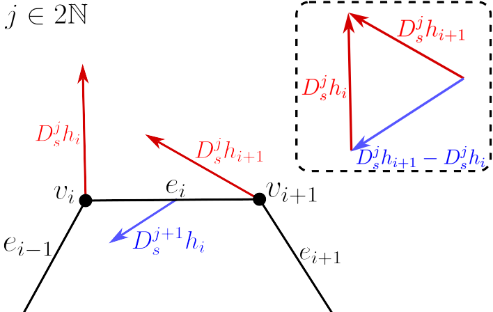
We now wish to define a Riemannian metric gm{g}^{m} on d×n\mathbb{R}^{d\times n}_{*}, which can be interpreted as a discretization of Gm{G}^{m}. First, we define some notation. Given a curve cd×nc\in\mathbb{R}^{d\times n}_{*} we denote our vertices as cic_{i} and let ei=ci+1cie_{i}=c_{i+1}-c_{i} denote the edge beginning at cic_{i} and ending at ci+1c_{i+1}. We also denote the average length of the two edges meeting at the vertex cic_{i} as μi=|ei|+|ei1|2\mu_{i}=\frac{|e_{i}|+|e_{i-1}|}{2}. Let hTcd×nh\in T_{c}\mathbb{R}^{d\times n}_{*} denote a tangent vector to cc with hih_{i} denoting the ii-th component of hh. To define our discrete metric gm{g}^{m} we will also need to define the jj-th discrete derivative at the iith vertex DsjhiD_{s}^{j}h_{i} using some ideas from discrete differential geometry [18, 19]. We define these recursively via

Ds0hi=hiDsj+1hi={DsjhiDsjhi1μij2Dsjhi+1Dsjhi|ei|j2.D_{s}^{0}h_{i}=h_{i}\qquad D_{s}^{j+1}h_{i}=\begin{cases}\frac{D_{s}^{j}h_{i}-D_{s}^{j}h_{i-1}}{\mu_{i}}\quad j\notin 2\mathbb{N}\\ \frac{D_{s}^{j}h_{i+1}-D_{s}^{j}h_{i}}{|e_{i}|}\quad j\in 2\mathbb{N}\end{cases}.

A visualization of this construction can be seen in Figure 1.

Refer to caption
Figure 1: A pictorial representation of the discrete derivative. The derivative DsjhD_{s}^{j}h can be seen here as a scaled first difference of Dsj1hD_{s}^{j-1}h.

This allows us to define some useful notation for something analogous to the mm-th order component of Gm{G}^{m}.

Definition 2.

For cd×nc\in\mathbb{R}^{d\times n}_{*} and h,kd×nh,k\in\mathbb{R}^{d\times n} we let

g˙cm(h,k):=i=1n(c)2m3Dsmhi,Dsmkiμi,m where μi,m={μim2+|ei|m2+\dot{{g}}_{c}^{m}(h,k):=\sum_{i=1}^{n}\ell(c)^{2m-3}\langle D_{s}^{m}h_{i},D_{s}^{m}k_{i}\rangle\mu_{i,m}\text{ where }\mu_{i,m}=\begin{cases}\mu_{i}\quad m\in 2\mathbb{Z}^{+}\\ |e_{i}|\quad m\notin 2\mathbb{Z}^{+}\end{cases}

and

gcm(h,k)=g˙c0(h,k)+g˙cm(h,k).{g}_{c}^{m}(h,k)=\dot{{g}}_{c}^{0}(h,k)+\dot{{g}}_{c}^{m}(h,k).

In the following lemma we justify the above notation and show the above defines a Riemannian metric on d×n\mathbb{R}^{d\times n}_{*}.

Lemma 3.

Let n3n\geq 3 and m0m\geq 0. Then gm{g}^{m} is a Riemannian metric on d×n\mathbb{R}^{d\times n}_{*}.

Proof.

We need to check non-degeneracy of the inner product and the smooth dependence on the base point cc. As gcm(h,h)g˙c0(h,h)g_{c}^{m}(h,h)\geq\dot{g}_{c}^{0}(h,h) it follows that if gcm(h,h)=0g_{c}^{m}(h,h)=0 then we also have g˙c0(h,h)=0\dot{g}_{c}^{0}(h,h)=0. As each edge length |ei||e_{i}| and μi\mu_{i} are nonzero for any cc, this can only happen if Ds0hi,Ds0hi=hi,hi=0\langle D_{s}^{0}h_{i},D_{s}^{0}h_{i}\rangle=\langle h_{i},h_{i}\rangle=0 for all ii. That implies hi=0h_{i}=0 for all ii. Thus for any mm, gcm(h,h)=0g_{c}^{m}(h,h)=0 implies h0h\equiv 0.

We next check that gcm{g}^{m}_{c} varies smoothly with respect to the base point cc. The only suspect term in the definition is |ei||e_{i}|. Varying cic_{i} in the uu direction yields the following:

u|ei|=uei|ei|u|ei1|=uei1|ei1|\frac{\partial}{\partial u}|e_{i}|=\frac{-u\cdot e_{i}}{|e_{i}|}\qquad\frac{\partial}{\partial u}|e_{i-1}|=\frac{u\cdot e_{i-1}}{|e_{i-1}|}

which implies the smoothness of the metric as |ei|>0|e_{i}|>0 for each ii of any curve in d×n\mathbb{R}^{d\times n}_{*}. ∎

In the next Lemma we will show that higher order metrics dominate lower order metrics, which will be of importance in the next section, where we will establish the main completeness results of the present article.

Lemma 4.

Let m1m\geq 1, cd×nc\in\mathbb{R}^{d\times n}_{*} and hd×nh\in\mathbb{R}^{d\times n}, then

g˙cm(h,h)14g˙cm+1(h,h).\dot{{g}}^{m}_{c}(h,h)\leq\frac{1}{4}\dot{{g}}^{m+1}_{c}(h,h). (3)
Proof.

The proof of this result is rather technical and we postpone it to the appendix. ∎

With these lemmas in hand, we arrive at a result concerning the main properties of the discrete Riemannian metric gmg^{m}, which parallels the statements of Lemma 1.

Lemma 5.

The metric gcm(h,k){g}^{m}_{c}(h,k) has the following properties:

  1. 1.

    For all n3n\geq 3, m0m\geq 0, gm{g}^{m} is invariant with respect to the action of n\frac{\mathbb{Z}}{n\mathbb{Z}} on d×n\mathbb{R}^{d\times n}_{*}, as well as rescaling, rotation, and translation. If jnj\in\frac{\mathbb{Z}}{n\mathbb{Z}}, λ+\lambda\in\mathbb{R}^{+}, RSO(d)R\in\operatorname{SO}(\mathbb{R}^{d}) and 𝐯d\mathbf{v}\in\mathbb{R}^{d}, then

    gcm(h,k)\displaystyle{g}_{c}^{m}(h,k) =gcjm(hj,kj)=gλcm(λh,λk)=g𝐯+cm(h,k)=gRcm(Rh,Rk).\displaystyle={g}_{c\circ j}^{m}(h\circ j,k\circ j)={g}_{\lambda c}^{m}(\lambda h,\lambda k)={g}_{\mathbf{v}+c}^{m}(h,k)={g}_{Rc}^{m}(Rh,Rk).
  2. 2.

    The metric gm(h,k){g}^{m}(h,k) is equivalent to any metric of the form

    g~m(h,k):=j=0mi=1naj(c)2j3Dsjhi,Dsjkiμi,m\widetilde{{g}}^{m}(h,k):=\sum_{j=0}^{m}\sum_{i=1}^{n}a_{j}\ell(c)^{2j-3}\langle D_{s}^{j}h_{i},D_{s}^{j}k_{i}\rangle\mu_{i,m}

    for a0,am>0a_{0},a_{m}>0 and aj0a_{j}\geq 0 for j=1,,m1j=1,\ldots,m-1 in the following sense: for some CC\in\mathbb{R}, all cImm(S1,d)c\in\operatorname{Imm}(S^{1},\mathbb{R}^{d}) and all hTcd×nd×nh\in T_{c}\mathbb{R}^{d\times n}_{*}\cong\mathbb{R}^{d\times n}

    1Cg~cm(h,h)gcm(h,h)Cg~cm(h,h).\frac{1}{C}\widetilde{{g}}^{m}_{c}(h,h)\leq{g}^{m}_{c}(h,h)\leq C\widetilde{{g}}^{m}_{c}(h,h).
Proof.

The proof of statement 1 is similar to the smooth case and we will not present the proof for translation, rotation, or scale invariance. The key difference is the action by n\frac{\mathbb{Z}}{n\mathbb{Z}}. Note gcm(h,k){g}_{c}^{m}(h,k) and gcjm(hj,kj){g}_{c\circ j}^{m}(h\circ j,k\circ j) sum over the exact same terms. Therefore, since |eij|=|ei+j||e_{i}\circ j|=|e_{i+j}| and μij=μi+j\mu_{i}\circ j=\mu_{i+j}, we see

g˙cjm(hj,kj)=i=1+jn+j(c)2m3Dsmhi,Dsmkiμi,m=i=1n(c)2m3Dsmhi,Dsmkiμi,m=g˙cm(h,k)\dot{{g}}_{c\circ j}^{m}(h\circ j,k\circ j)=\sum_{i=1+j}^{n+j}\ell(c)^{2m-3}\langle D_{s}^{m}h_{i},D_{s}^{m}k_{i}\rangle\mu_{i,m}=\sum_{i=1}^{n}\ell(c)^{2m-3}\langle D_{s}^{m}h_{i},D_{s}^{m}k_{i}\rangle\mu_{i,m}=\dot{{g}}_{c}^{m}(h,k)

where the center equality is due to the fact that ii belongs to n\frac{\mathbb{Z}}{n\mathbb{Z}} so that the i=1i=1 term of the sum is identical to the i=n+1i=n+1 term.

Statement 2 largely follows via Lemma 4. Given our g~m\widetilde{{g}}^{m}, it allows us to collect all our coefficients into g˙0\dot{g}^{0} and g˙m\dot{g}^{m} terms alone to form a g^m\widehat{{g}}^{m} with

a0g˙c0(h,h)+amg˙cm(h,h)g~cm(h,h)g^cm(h,h).a_{0}\dot{{g}}^{0}_{c}(h,h)+a_{m}\dot{{g}}^{m}_{c}(h,h)\leq\widetilde{{g}}^{m}_{c}(h,h)\leq\widehat{{g}}^{m}_{c}(h,h).

As g^cm(h,h)=a^0g˙0(h,h)+a^mg˙m(h,h)\widehat{{g}}^{m}_{c}(h,h)=\hat{a}_{0}\dot{{g}}^{0}(h,h)+\hat{a}_{m}\dot{{g}}^{m}(h,h) for some a0a^0a_{0}\leq\hat{a}_{0} and ama^ma_{m}\leq\hat{a}_{m}. Note also that

min(a^0,a^m)gcm(h,h)g^cm(h,h)max(a^0,a^m)gcm(h,h)\min(\hat{a}_{0},\hat{a}_{m}){g}^{m}_{c}(h,h)\leq\widehat{{g}}^{m}_{c}(h,h)\leq\max(\hat{a}_{0},\hat{a}_{m}){g}^{m}_{c}(h,h)

and similar for a0g˙c0(h,h)+amg˙cm(h,h)a_{0}\dot{{g}}^{0}_{c}(h,h)+a_{m}\dot{{g}}^{m}_{c}(h,h). Thus we may write

1Cgcm(h,h)min(a0,am)gcm(h,h)g~cm(h,h)max(a^0,a^m)gcm(h,h)Cgcm(h,h)\frac{1}{C}{g}^{m}_{c}(h,h)\leq\min(a_{0},a_{m}){g}^{m}_{c}(h,h)\leq\widetilde{{g}}^{m}_{c}(h,h)\leq\max(\hat{a}_{0},\hat{a}_{m}){g}^{m}_{c}(h,h)\leq C{g}^{m}_{c}(h,h)

for

C=max(1min(a0,am),max(a^0,a^m)).C=\max\left(\frac{1}{\min(a_{0},a_{m})},\max(\hat{a}_{0},\hat{a}_{m})\right).

Via multiplication by CC we find gcm(h,h)Cg~cm(h,h){g}^{m}_{c}(h,h)\leq C\widetilde{{g}}^{m}_{c}(h,h) and via division we find 1Cg~cm(h,h)gcm(h,h).\frac{1}{C}\widetilde{{g}}^{m}_{c}(h,h)\leq{g}^{m}_{c}(h,h). Together these give the desired statement

1Cg~cm(h,h)gcm(h,h)Cg~cm(h,h).\frac{1}{C}\widetilde{{g}}^{m}_{c}(h,h)\leq{g}^{m}_{c}(h,h)\leq C\widetilde{{g}}^{m}_{c}(h,h).

We have seen that this discrete metric shares several properties with its infinite dimensional counterpart. In the following proposition we show that we are indeed justified in referring to it as a discretization of Gm{G}^{m}:

Prop. 1.

Let n3n\geq 3 and for i=0,,n1i=0,\ldots,n-1 let θi=in\theta_{i}=\frac{i}{n}. Let cImm(S1,d)c\in\operatorname{Imm}(S^{1},\mathbb{R}^{d}) and h,kTcImm(S1,d)h,k\in T_{c}\operatorname{Imm}(S^{1},\mathbb{R}^{d}). Define c~n=(c(θ1),c(θ2),,c(θn))d×n\tilde{c}_{n}=(c(\theta_{1}),c(\theta_{2}),\ldots,c(\theta_{n}))\in\mathbb{R}^{d\times n}_{*}. Similarly define h~n\tilde{h}_{n} and k~n\tilde{k}_{n} using h,kh,k. Then

limngc~nm(h~n,k~n)=Gcm(h,k)\lim_{n\to\infty}{g}^{m}_{\tilde{c}_{n}}(\tilde{h}_{n},\tilde{k}_{n})={G}^{m}_{c}(h,k)
Proof.

To prove this statement we will make use of a technical result regarding the approximation of derivatives, which we postponed to the appendix, cf. Lemma 8. We first define several relevant operators and notational items. Given cImm(S1,d)c\in\operatorname{Imm}(S^{1},\mathbb{R}^{d}) we let μ^c,n,m=|In1(c)|\widehat{\mu}_{c,n,m}=|I_{n}^{1}(c)| if mm is even and μ^c,n,m=|In1(c)|+|I~n1(c)|2\widehat{\mu}_{c,n,m}=\frac{|I_{n}^{1}(c)|+|\widetilde{I}_{n}^{1}(c)|}{2} if mm is odd. Now, for a given cImm(S1,d)c\in\operatorname{Imm}(S^{1},\mathbb{R}^{d}) and n3n\in\mathbb{Z}_{\geq 3} define 𝒟c,n,m\mathcal{D}_{c,n,m} via the following recursive formula

𝒟c,n,0(f)=In0(f)𝒟c,n,m(f)={I~n1(Dc,n,m1(f))μ^c,n,mm2+In1(Dc,n,m1(f))μ^c,n,mm2+.\mathcal{D}_{c,n,0}(f)=I^{0}_{n}(f)\qquad\mathcal{D}_{c,n,m}(f)=\begin{cases}\frac{\widetilde{I}^{1}_{n}(D_{c,n,m-1}(f))}{\widehat{\mu}_{c,n,m}}\quad m\in 2\mathbb{Z}^{+}\\ \frac{I^{1}_{n}(D_{c,n,m-1}(f))}{\widehat{\mu}_{c,n,m}}\quad m\notin 2\mathbb{Z}^{+}\end{cases}.

Note that all the nn cancel in these definitions once expanded as at each step we introduce a factor of nn in both the numerator and denominator. Next define n(c)\ell_{n}(c) as i=1n|c(θi+1)c(θi)|\sum_{i=1}^{n}|c(\theta_{i+1})-c(\theta_{i})|. With these in hand we define:

Fm(h,k,c,n,θ)=n(c)2m3𝒟c,n,m(h),𝒟c,n,m(k)μ^c,n,m.F_{m}(h,k,c,n,\theta)=\ell_{n}(c)^{2m-3}\left\langle\mathcal{D}_{c,n,m}(h),\mathcal{D}_{c,n,m}(k)\right\rangle\widehat{\mu}_{c,n,m}.

We prove the proposition in two steps

Claim 1.

S1Fm(h,k,c,n,θ)𝑑θ=g˙c~nm(h~n,k~n)\int_{S^{1}}F_{m}(h,k,c,n,\theta)d\theta=\dot{{g}}^{m}_{\widetilde{c}_{n}}(\widetilde{h}_{n},\widetilde{k}_{n})

We expand to

S1Fm(h,k,c,n,θ)𝑑θ=S1n(c)2m3𝒟c,n,m(h),𝒟c,n,m(k)μ^c,n,m𝑑θ\int_{S^{1}}F_{m}(h,k,c,n,\theta)d\theta=\int_{S^{1}}\ell_{n}(c)^{2m-3}\left\langle\mathcal{D}_{c,n,m}(h),\mathcal{D}_{c,n,m}(k)\right\rangle\widehat{\mu}_{c,n,m}d\theta

and note that the integrand on the right is constant on each interval [θi,θi+1)[\theta_{i},\theta_{i+1}) as n\ell_{n} is constant with respect to θ\theta and each of 𝒟c,n,m(h),𝒟c,n,m(k)\mathcal{D}_{c,n,m}(h),\mathcal{D}_{c,n,m}(k), and μc,n,m{\mu}_{c,n,m} are constant on such intervals. Thus for some 𝒟~c,n,m,i(h),𝒟~c,n,m,i(k)d\widetilde{\mathcal{D}}_{c,n,m,i}(h),\widetilde{\mathcal{D}}_{c,n,m,i}(k)\in\mathbb{R}^{d} we can write either

S1Fm(h,k,c,n,θ)𝑑θ=i=1nn(c)2m31n𝒟~c,n,m,i(h),𝒟~c,n,m,i(k)|n(c(θi+1)c(θi))|\int_{S^{1}}F_{m}(h,k,c,n,\theta)d\theta=\sum_{i=1}^{n}\ell_{n}(c)^{2m-3}\frac{1}{n}\left\langle\widetilde{\mathcal{D}}_{c,n,m,i}(h),\widetilde{\mathcal{D}}_{c,n,m,i}(k)\right\rangle|n(c(\theta_{i+1})-c(\theta_{i}))|

or

=i=1nn(c)2m31n𝒟~c,n,m,i(h),𝒟~c,n,m,i(k)|n(c(θi+1)c(θi))|+|n(c(θi)c(θi1))|2=\sum_{i=1}^{n}\ell_{n}(c)^{2m-3}\frac{1}{n}\left\langle\widetilde{\mathcal{D}}_{c,n,m,i}(h),\widetilde{\mathcal{D}}_{c,n,m,i}(k)\right\rangle\frac{|n(c(\theta_{i+1})-c(\theta_{i}))|+|n(c(\theta_{i})-c(\theta_{i-1}))|}{2}

depending on the parity of mm. Note all nn cancel and we can rewrite further to either

i=1nn(c)2m3𝒟~c,n,m,i(h),𝒟~c,n,m,i(k)|ei|\sum_{i=1}^{n}\ell_{n}(c)^{2m-3}\left\langle\widetilde{\mathcal{D}}_{c,n,m,i}(h),\widetilde{\mathcal{D}}_{c,n,m,i}(k)\right\rangle|e_{i}|

for odd mm or

i=1nn(c)2m3𝒟~c,n,m,i(h),𝒟~c,n,m,i(k)μi\sum_{i=1}^{n}\ell_{n}(c)^{2m-3}\left\langle\widetilde{\mathcal{D}}_{c,n,m,i}(h),\widetilde{\mathcal{D}}_{c,n,m,i}(k)\right\rangle\mu_{i}

for even mm. Thus the only thing that remains to be shown for this first claim is that these 𝒟~\widetilde{\mathcal{D}} terms are our discrete DsD_{s} derivatives of h~n\widetilde{h}_{n} and k~n\widetilde{k}_{n}. This is clear for m=0m=0 as In0(h)I^{0}_{n}(h) is simply the step function taking on the value h~n,i=h(in)\widetilde{h}_{n,i}=h\left(\frac{i}{n}\right) on [θi,θi+1)[\theta_{i},\theta_{i+1}). For m>0m>0 we see either

𝒟~c,n,m,i(h)=𝒟~c,n,m1,i+1(h)𝒟~c,n,m1,i(h)|ei|\widetilde{\mathcal{D}}_{c,n,m,i}(h)=\frac{\widetilde{\mathcal{D}}_{c,n,m-1,i+1}(h)-\widetilde{\mathcal{D}}_{c,n,m-1,i}(h)}{|e_{i}|}

or

𝒟~c,n,m,i(h)dθ=𝒟~c,n,m1,i(h)𝒟~c,n,m1,i1(h)μi\widetilde{\mathcal{D}}_{c,n,m,i}(h)d\theta=\frac{\widetilde{\mathcal{D}}_{c,n,m-1,i}(h)-\widetilde{\mathcal{D}}_{c,n,m-1,i-1}(h)}{\mu_{i}}

so that by induction it follows that these really do correspond to the discrete derivatives as 𝒟~c,n,m,i(h)\widetilde{\mathcal{D}}_{c,n,m,i}(h) relates to 𝒟~c,n,m1,j(h)\widetilde{\mathcal{D}}_{c,n,m-1,j}(h) identically to how DsmhiD_{s}^{m}h_{i} relates to Dsm1hjD_{s}^{m-1}h_{j}.
The second step is easier by comparison. We have shown that S1Fm()=g˙c~nm()\int_{S^{1}}F_{m}(\dotsm)=\dot{{g}}_{\tilde{c}_{n}}^{m}(\dotsm). We next need to show how the limit of FmF_{m} is related to G˙cm(h,k)=2m3Dsmh,Dsmk|c|\dot{{G}}^{m}_{c}(h,k)=\ell^{2m-3}\langle D_{s}^{m}h,D_{s}^{m}k\rangle|c^{\prime}| which will allow us to relate gm{g}^{m} and Gm{G}^{m}.

Claim 2.

limnFm(h,k,c,n,θ)LG˙cm(h,k)\displaystyle{\lim_{n\to\infty}F_{m}(h,k,c,n,\theta)\overset{L^{\infty}}{\to}\dot{{G}}^{m}_{c}(h,k)}

By Lemma 8 it follows that

limn𝒟c,n,m(f)Dsm(f)L0andlimnμ^c,n,m|c|L0.\lim_{n\to\infty}\left\|\mathcal{D}_{c,n,m}(f)-D_{s}^{m}(f)\right\|_{L^{\infty}}\to 0\quad\text{and}\quad\lim_{n\to\infty}\|\hat{\mu}_{c,n,m}-|c^{\prime}|\|_{L^{\infty}}\to 0.

It is also clear that limnn(c)(c)\lim_{n\to\infty}\ell_{n}(c)\to\ell(c) as our curves are rectifiable. Now

limnFm(h,k,c,n,θ)G˙cm(h,k)L0.\lim_{n\to\infty}\|F_{m}(h,k,c,n,\theta)-\dot{{G}}^{m}_{c}(h,k)\|_{L^{\infty}}\to 0.

This implies that limnFm()\displaystyle{\lim_{n\to\infty}F_{m}(\dotsm)} is equal to G˙cm(h,k)\dot{{G}}^{m}_{c}(h,k) almost everywhere, and we may join our claims together via

S1G˙cm(h,k)𝑑θ=S1limnFm()dθ=limnS1Fm()𝑑θ=limng˙c~nm(h~n,k~n),\int_{S^{1}}\dot{{G}}^{m}_{c}(h,k)d\theta=\int_{S^{1}}\lim_{n\to\infty}F_{m}(\dotsm)d\theta\overset{*}{=}\lim_{n\to\infty}\int_{S^{1}}F_{m}(\dotsm)d\theta=\lim_{n\to\infty}\dot{{g}}^{m}_{\tilde{c}_{n}}(\tilde{h}_{n},\tilde{k}_{n}),

where * follows by the Lebesgue dominated convergence theorem as we can bound the integrand almost everywhere by the constant function on S1S^{1} equal to G˙cm(h,k)L\|\dot{{G}}^{m}_{c}(h,k)\|_{L^{\infty}}. By linearity it follows

Gcm(h,k)=limngc~nm(h~n,k~n){G}^{m}_{c}(h,k)=\lim_{n\to\infty}{g}^{m}_{\tilde{c}_{n}}(\tilde{h}_{n},\tilde{k}_{n})

which completes the proof. ∎

4 Completeness Results

In this section we will prove the main theoretical result of the present article, namely we will show that the finite dimensional manifolds (d×n,gm)(\mathbb{R}^{d\times n}_{*},{g}^{m}) indeed capture the completeness properties of the space of smooth, regular curves equipped with the class of reparametrization invariant Sobolev metrics Gm{G}^{m}, i.e., we will prove the following theorem:

Theorem 2 (Completeness of the gm{g}^{m}-metric).

Let m2m\geq 2, n3n\geq 3 and d2d\geq 2. Then the space (d×n,gm)(\mathbb{R}^{d\times n}_{*},{g}^{m}) is metrically and geodesically complete. Furthermore, for any two points in d×n\mathbb{R}^{d\times n}_{*} there exists a minimizing geodesic, i.e., (d×n,gm)(\mathbb{R}^{d\times n}_{*},{g}^{m}) is geodesically convex.

This theorem can readily be seen as a discrete equivalent to the above Theorem 1 from the smooth case. As d×n\mathbb{R}^{d\times n}_{*} is finite dimensional, Hopf-Rinow implies we need only show metric completeness and that both geodesic completeness and geodesic convexity follow automatically. The requirement that d2d\geq 2 is due to the fact that 1×n\mathbb{R}^{1\times n}_{*} is not connected and thus Hopf-Rinow does not apply. We begin by proving a useful lemma

Lemma 6.

Let (,g)(\mathcal{M},g) be a possibly infinite dimensional manifold. (,g)(\mathcal{M},g) is metrically incomplete if and only if there exists a path γ:[0,1)\gamma:[0,1)\to\mathcal{M}, such that

  1. 1.

    γ(t)\gamma(t)\in\mathcal{M} for 0t<10\leq t<1;

  2. 2.

    limt1γ(t)\displaystyle{\lim_{t\to 1}}\gamma(t) does not exist in (,g)(\mathcal{M},g);

  3. 3.

    the length of γ\gamma (w.r.t. gg) is finite, i.e., Lg(γ)<L_{g}(\gamma)<\infty.

Proof.

We first assume incompleteness. As \mathcal{M} is metrically incomplete there exists some Cauchy sequence xnx_{n} that fails to converge in the space. Without loss of generality we can assume ndg(xn,xn+1)<\sum_{n}^{\infty}d_{g}(x_{n},x_{n+1})<\infty. This is since we can always find a Cauchy sub-sequence of our Cauchy sequence with this property. To construct such a sub-sequence we perform the following procedure: if, under our Cauchy conditions, for all n,mN(i)n,m\geq N(i) we have dg(xn,xm)<110id_{g}(x_{n},x_{m})<\frac{1}{10^{i}} then we define our sub-sequence as {xN(i)}i{xn}\{x_{N(i)}\}_{i\in\mathbb{N}}\subset\{x_{n}\}. The length i=1dg(xN(i),xN(i+1))\sum_{i=1}^{\infty}d_{g}(x_{N(i)},x_{N(i+1)}) of this sub-sequence is bounded above by 19\frac{1}{9} by construction as i=1dg(xN(i),xN(i+1))<i=1110i=19\sum_{i=1}^{\infty}d_{g}(x_{N(i)},x_{N(i+1)})<\sum_{i=1}^{\infty}\frac{1}{10^{i}}=\frac{1}{9}.

While we cannot guarantee paths lying in the space between the elements of our sequence that realize their distances, we can have a collection of paths γn\gamma_{n} going from xnx_{n} to xn+1x_{n+1} with a length <dg(xn,xn+1)+12n<d_{g}(x_{n},x_{n+1})+\frac{1}{2^{n}} lying within the space so that the overall distance of γ=γ1γ2γ3\gamma=\gamma_{1}*\gamma_{2}*\gamma_{3}*\dotsm will have a total length L(γ)<1+n=1dg(xn,xn+1)L(\gamma)<1+\sum_{n=1}^{\infty}d_{g}(x_{n},x_{n+1}). Here * denotes usual path composition. γ\gamma is then of finite length with limt1γ(t)\lim_{t\to 1}\gamma(t)\notin\mathcal{M} and γ(t)\gamma(t)\in\mathcal{M} for 0t<10\leq t<1.

On the other hand, assuming such a path, we wish to show we have a Cauchy sequence that does not converge with respect to our metric. Without loss of generality assume γ\gamma is traversed with constant speed. If aa and bb are points on our curve, then let d(a,b)d(a,b) be the length of the subsegment of gamma with endpoints γ(a),γ(b)\gamma(a),\gamma(b). As γ\gamma is traversed with constant speed we see d(ti,tj)=Lg(γ)|titj|d(t_{i},t_{j})=L_{g}(\gamma)|t_{i}-t_{j}|. The distance of γ(ti)\gamma(t_{i}) and γ(tj)\gamma(t_{j}) along γ\gamma is not necessarily equal with the distance of these points in the space, but if dgd_{g} is the metric distance, then dg(γ(ti),γ(tj))d(ti,tj)=Lg(γ)|titj|d_{g}(\gamma(t_{i}),\gamma(t_{j}))\leq d(t_{i},t_{j})=L_{g}(\gamma)|t_{i}-t_{j}|. Set tn=11nt_{n}=1-\frac{1}{n} noting that this sequence (tn)(t_{n}) is a Cauchy sequence in the reals. The distances between a pair of these points is dg(γ(ti),γ(tj))Lg(γ)|titj|d_{g}(\gamma(t_{i}),\gamma(t_{j}))\leq L_{g}(\gamma)|t_{i}-t_{j}|. Now given any ε>0\varepsilon>0 we have some NN so that for all i,j>Ni,j>N we have |titj|<εLg(γ)|t_{i}-t_{j}|<\frac{\varepsilon}{L_{g}(\gamma)} so that dg(γ(ti),γ(tj))<εd_{g}(\gamma(t_{i}),\gamma(t_{j}))<\varepsilon. This makes γ(tn)\gamma(t_{n}) a Cauchy sequence in \mathcal{M}, but (tn)(t_{n}) converges to 1 so this Cauchy sequence does not converge in our space:

limnγ(tn)=limt1γ(t).\lim_{n\to\infty}\gamma(t_{n})=\lim_{t\to 1}\gamma(t)\notin\mathcal{M}.

Thus our space is not metrically complete. ∎

Corollary 1.

Let (,g)(\mathcal{M},g) and (,g)(\mathcal{M},g^{*}) be two Riemannian manifolds such that for all pp\in\mathcal{M}, r+r\in\mathbb{R}^{+}, qBg(p,r)q\in B_{g^{*}}(p,r) and hTqh\in T_{q}\mathcal{M} we have gq(h,h)Cgq(h,h)g_{q}(h,h)\leq Cg^{*}_{q}(h,h) for some constant CC potentially dependent on our choice of pp and rr. Then if (,g)(\mathcal{M},g) is metrically complete so is (,g)(\mathcal{M},g^{*}).

Proof.

Suppose (,g)(\mathcal{M},g^{*}) were incomplete while (,g)(\mathcal{M},g) were complete. By Lemma 6 there exists a path γ(t)\gamma(t) such that γ(t)\gamma(t)\in\mathcal{M} for t[0,1)t\in[0,1) and limt1γ(t)\lim_{t\to 1}\gamma(t)\notin\mathcal{M} with finite length under gg^{*} and no similar finite length path exists under gg. Let rr_{*} be such that Lg(γ)=r0<r<L_{g^{*}}(\gamma)=r_{0}<r_{*}<\infty. Note gγ(t)(h,h)Cgγ(t)(h,h)g_{\gamma(t)}(h,h)\leq Cg^{*}_{\gamma(t)}(h,h) since γ(t)B(γ0,r)\gamma(t)\in B(\gamma_{0},r_{*}) for all t[0,1)t\in[0,1). We thus have

Lg(γ(t))\displaystyle L_{g}(\gamma(t)) =01gγ(t)(Dtγ(t),Dtγ(t))𝑑t\displaystyle=\int_{0}^{1}\sqrt{g_{\gamma(t)}(D_{t}\gamma(t),D_{t}\gamma(t))}dt
<C01gγ(t)(Dtγ(t),Dtγ(t))𝑑t=CLg(γ(t))=r0C<\displaystyle<\sqrt{C}\int_{0}^{1}\sqrt{g^{*}_{\gamma(t)}(D_{t}\gamma(t),D_{t}\gamma(t))}dt=\sqrt{C}L_{g^{*}}(\gamma(t))=r_{0}\sqrt{C}<\infty

This is a contradiction as it implies γ\gamma is of finite length in (,g)(\mathcal{M},g). ∎

With this in hand, we are now ready to prove Theorem 2.

Proof of Theorem 2.

Corollary 1 and Lemma 4 together imply we need only consider the metric completeness of d×n\mathbb{R}^{d\times n}_{*} equipped with g2{g}^{2}. Via Lemma 6 it is sufficient to show any path γ:[0,1)d×n\gamma:[0,1)\to\mathbb{R}^{d\times n}_{*} with Lg2(γ)<L_{{g}^{2}}(\gamma)<\infty has limt1γ(t)d×n\lim_{t\to 1}\gamma(t)\in\mathbb{R}^{d\times n}_{*} to show metric completeness of (d×n,g2)(\mathbb{R}^{d\times n}_{*},{g}^{2}). There are three cases to consider, as there are three ways for limt1γ(t)\lim_{t\to 1}\gamma(t) to not exist in d×n\mathbb{R}^{d\times n}_{*}:

  1. (Case 1)

    Some point escapes to infinity, edge lengths stay greater than 0, and curve length does not become infinite:
    j\exists j such that limt1|γj|=\lim_{t\to 1}|\gamma_{j}|=\infty, (γ(t))<\ell(\gamma(t))<\infty and |ei|>0,i,t[0,1]|e_{i}|>0,\forall i,\forall t\in[0,1].

  2. (Case 2)

    Some edges but not all edges shrink to length 0:
    i:limt1|ei|=0\exists i:\lim_{t\to 1}|e_{i}|=0 and j:|ej|>0,t[0,1].\exists j:|e_{j}|>0,\forall t\in[0,1].

  3. (Case 3)

    All edges shrink to length 0 or curve length is unbounded:
    limt1(γ(t))=0\lim_{t\to 1}\ell(\gamma(t))=0 or limt1(γ(t))=\lim_{t\to 1}\ell(\gamma(t))=\infty

Below we make use of the following estimates

|Dt|γ(t)i|||Dtγ(t)i||Dt|ei|||Dtei||Dt(γ(t))|i=1n|Dtei|.\left|D_{t}|\gamma(t)_{i}|\right|\leq|D_{t}\gamma(t)_{i}|\qquad\left|D_{t}|e_{i}|\right|\leq|D_{t}e_{i}|\qquad\left|D_{t}\ell(\gamma(t))\right|\leq\sum_{i=1}^{n}|D_{t}e_{i}|.

The first two of these are derived from the same general pattern:

±Dt|v|=±Dtv,v|v|=Dtv,±v|v||Dtv|\pm D_{t}|v|=\pm\frac{\langle D_{t}v,v\rangle}{|v|}=\frac{\langle D_{t}v,\pm v\rangle}{|v|}\leq|D_{t}v|

as ±v|v|\frac{\pm v}{|v|} is a unit vector. The third inequality comes from noting |Dt(γ(t))|=|i=1nDt|ei||\left|D_{t}\ell(\gamma(t))\right|=\left|\sum_{i=1}^{n}D_{t}|e_{i}|\right| and using the second inequality.

Now we proceed by cases:
(Case 1): We appeal to g˙0\dot{{g}}^{0}. Let γ(t)j\gamma(t)_{j} be the vertex escaping

Łg2(γ(t))\displaystyle\L_{{g}^{2}}(\gamma(t)) 01i=1n1(γ(t))3|Dtγ(t)i|2μi𝑑t011(γ(t))3/2|Dtγ(t)j|μj𝑑tM01|Dtγ(t)j|𝑑t\displaystyle\geq\int_{0}^{1}\sqrt{\sum_{i=1}^{n}\frac{1}{\ell(\gamma(t))^{3}}|D_{t}\gamma(t)_{i}|^{2}\mu_{i}}dt\geq\int_{0}^{1}\frac{1}{\ell(\gamma(t))^{3/2}}|D_{t}\gamma(t)_{j}|\sqrt{\mu_{j}}dt\geq M\int_{0}^{1}|D_{t}\gamma(t)_{j}|dt
M01|Dt(|γ(t)j|)|𝑑tM|01Dt(|γ(t)j|)𝑑t|=M|limt|γ(t)j||γ(0)j|<|=\displaystyle\geq M\int_{0}^{1}\left|D_{t}(|\gamma(t)_{j}|)\right|dt\geq M\left|\int_{0}^{1}D_{t}(|\gamma(t)_{j}|)dt\right|=M\left|\underset{\infty}{\underbrace{\lim_{t\to\infty}|\gamma(t)_{j}|}}-\underset{<\infty}{\underbrace{|\gamma(0)_{j}|}}\right|=\infty

where M=mini,tμi(γ(t))3M=\min_{i,t}\sqrt{\frac{\mu_{i}}{\ell(\gamma(t))^{3}}}.
(Case 2): We appeal to g˙2\dot{{g}}^{2}. Let eke_{k} be an edge shrinking to length 0 such that ek1e_{k-1} is not shrinking to length 0. Such a pair of consecutive edges must exist, as we have edges shrinking to length zero and others not doing so, these subsets of our edges must meet at some vertex γ(t)k\gamma(t)_{k}.

Łg2(c)\displaystyle\L_{{g}^{2}}(c)\geq 01(γ(t))|Dtek|ek|Dtek1|ek1||1μi𝑑tM|01|Dtek|ek|||Dtek1|ek1||dt|\displaystyle\int_{0}^{1}\sqrt{\ell(\gamma(t))}\left|\frac{D_{t}e_{k}}{|e_{k}|}-\frac{D_{t}e_{k-1}}{|e_{k-1}|}\right|\frac{1}{\sqrt{\mu_{i}}}dt\geq M\left|\int_{0}^{1}\left|\frac{D_{t}e_{k}}{|e_{k}|}\right|-\left|\frac{D_{t}e_{k-1}}{|e_{k-1}|}\right|dt\right|
\displaystyle\geq M|01|Dtek|ek||dt01|Dtek1|ek1||dt|M|01|Dt|ek||ek||dt01|Dtek1|ek1||dt|\displaystyle M\left|\int_{0}^{1}\left|\frac{D_{t}e_{k}}{|e_{k}|}\right|dt-\int_{0}^{1}\left|\frac{D_{t}e_{k-1}}{|e_{k-1}|}\right|dt\right|\geq M\left|\int_{0}^{1}\left|\frac{D_{t}|e_{k}|}{|e_{k}|}\right|dt-\int_{0}^{1}\left|\frac{D_{t}e_{k-1}}{|e_{k-1}|}\right|dt\right|
M||01Dt|ek||ek|𝑑t|01|Dtek1|ek1||𝑑t|M||[ln(|ek|)]01|01|Dtek1|ek1||𝑑t<|=\displaystyle\geq M\left|\left|\int_{0}^{1}\frac{D_{t}|e_{k}|}{|e_{k}|}dt\right|-\int_{0}^{1}\left|\frac{D_{t}e_{k-1}}{|e_{k-1}|}\right|dt\right|\geq M\Bigg{|}\underset{\infty}{\underbrace{\Big{|}\left[\ln\left(|e_{k}|\right)\right]_{0}^{1}\Big{|}}}-\underset{<\infty}{\underbrace{\int_{0}^{1}\left|\frac{D_{t}e_{k-1}}{|e_{k-1}|}\right|dt}}\Bigg{|}=\infty

where M=mini,t(γ(t))μiM=\min_{i,t}\sqrt{\frac{\ell(\gamma(t))}{\mu_{i}}}.
(Case 3): We appeal to g˙1\dot{{g}}^{1}.

Łg2(γ(t))\displaystyle\L_{{g}^{2}}(\gamma(t)) CŁg1(γ(t))C01i=1n|Dtei|2(γ(t))|ei|𝑑tC01|Dtei|(γ(t))𝑑tfor each i\displaystyle\geq C\L_{{g}^{1}}(\gamma(t))\geq C\int_{0}^{1}\sqrt{\sum_{i=1}^{n}\frac{|D_{t}e_{i}|^{2}}{\ell(\gamma(t))|e_{i}|}}dt\geq C\int_{0}^{1}\frac{|D_{t}e_{i}|}{\ell(\gamma(t))}dt\quad\text{for each }i
Łg2(γ(t))\displaystyle\L_{{g}^{2}}(\gamma(t)) Cni=1n01|Dtei|(γ(t))𝑑t=Cn01i=1n|Dtei|(γ(t))dtCn01|Dt(γ(t))|(γ(t))𝑑t\displaystyle\overset{*}{\geq}\frac{C}{n}\sum_{i=1}^{n}\int_{0}^{1}\frac{|D_{t}e_{i}|}{\ell(\gamma(t))}dt=\frac{C}{n}\int_{0}^{1}\sum_{i=1}^{n}\frac{|D_{t}e_{i}|}{\ell(\gamma(t))}dt\geq\frac{C}{n}\int_{0}^{1}\frac{\left|D_{t}\ell(\gamma(t))\right|}{\ell(\gamma(t))}dt
Cn|01Dt(γ(t))(γ(t))𝑑t|=Cn|[ln((γ(t)))]01|=\displaystyle\geq\frac{C}{n}\left|\int_{0}^{1}\frac{D_{t}\ell(\gamma(t))}{\ell(\gamma(t))}dt\right|=\frac{C}{n}\left|\left[\ln\left(\ell(\gamma(t))\right)\right]_{0}^{1}\right|=\infty

The \geq marked * comes from the fact that the average of several underestimates is itself an underestimate.

5 Geodesics, curvature and a comparison to Kendall’s shape space

In this section we will further demonstrate the behavior of these geometries by presenting selected examples of geodesics for different choices of metrics. Finally, we will consider the special case of planar triangles, where we will compare the discrete Sobolev metrics defined in this paper with Kendall’s shape metric; it is well known that under Kendall’s metric the space of planar triangles reduces to a round sphere [22].

All numerical examples were obtained using the programming language Python, where we implemented both the Riemannian exponential map (and the Riemannian log map) by solving the the geodesic initial value problem (and boundary value problem, resp.).

Refer to caption
Figure 2: Riemannian exponential map w.r.t. to the metric g2{g}^{2}.

The geodesic initial value problem:

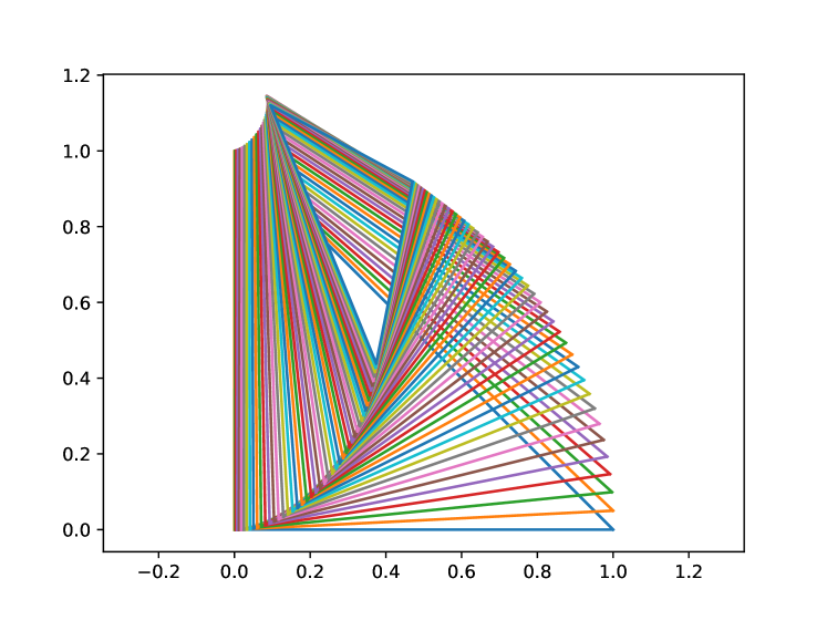
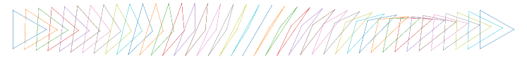
To approximate the Riemannian exponential map we calculate the Christoffel symbols using the automatic differentiation capabilities of pytorch. This in turn allows us to approximate the exponential map using a simple one-step Euler method. In Figure 2 one can see an approximated geodesic computed with initial conditions consisting of a right triangle (0,0),(0,1),(1,0)(0,0),(0,1),(1,0) and an initial velocity of (0,1)(0,1) on the third vertex and zero elsewhere. We note that an initial velocity which is non-zero only on a single vertex immediately puts multiple vertices in motion.

The geodesic boundary value problem:

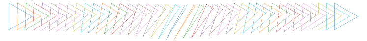
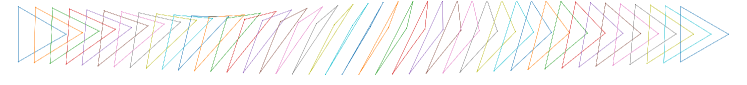
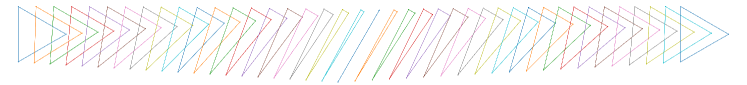
To approximate the Riemannian log map we employ a path-straigthening algorithm; i.e., we minimize the Riemannian energy over paths of curves starting at c0c_{0} and ending at c1c_{1}, approximated using a fixed (finite) number of intermediate curves. Thereby, we reduce the approximation of the Riemannian log map to a finite dimensional, unconstrained minimization problem, which we tackle using the scipy implementation of L-BFGS-B, where we use a simple linear interpolation as initialization. In particular, for higher order metrics the algorithm can fail if the initialization leaves the space of PL immersions, as the metric is undefined for curves that are not in d×n\mathbb{R}^{d\times n}_{*}. To fix this issue it is possible to add a small amount of noise to the vertices of the initialization. We present two different examples of solutions to the geodesic boundary value problem in Figure 3.

Refer to caption
Refer to caption
Figure 3: Examples of solutions to the geodesic boundary value problem w.r.t. to the metric g2{g}^{2}. First line: from a hexagon to a spiked figure. Second line: from the spiked figure to a blunt one.

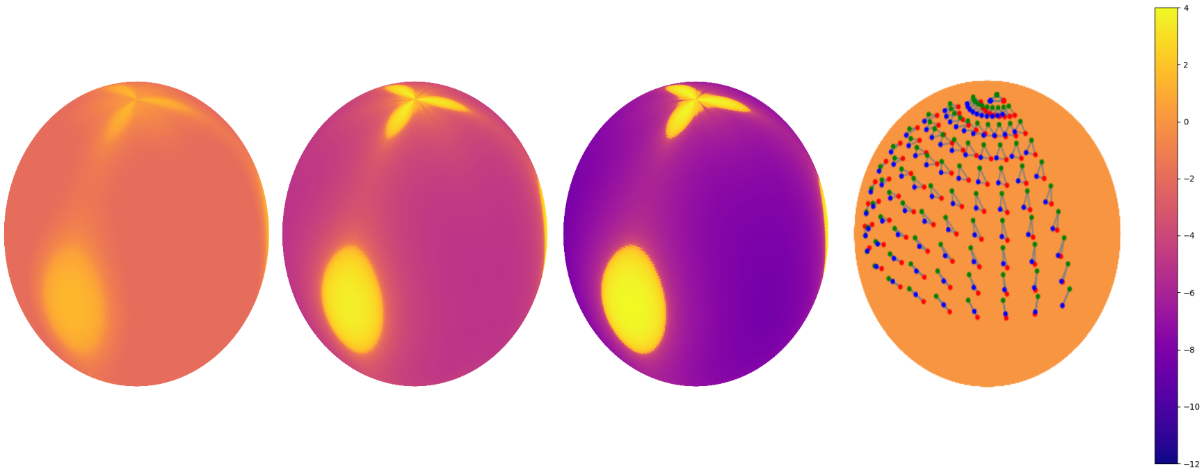
Gaussian Curvature of the Space of Triangles and Kendall’s shape metric:

A prudent comparison of the discrete metrics described in this work is with the Kendall metrics of discrete shapes, which may be defined on the same space. Comparing the geodesics with respect to these metrics also highlights the nature of our completeness result.

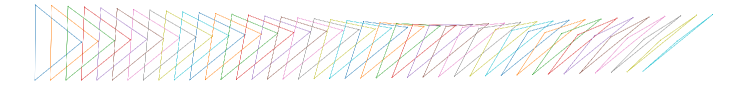
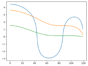
We start by restricting ourselves to the space of triangles 2×3\mathbb{R}^{2\times 3}_{*} modulo the actions of rotation, translation, and scale. This space can be identified with the surface of a sphere with three punctures (the punctures correspond to degenerate triangles in which two vertices coincide) and when equipped with the Kendall metric [22], this space is famously isometric to the punctured sphere and has constant Gaussian curvature. In Figure 4, we display boundary value geodesics with respect to the Kendall metric as well as for the discrete Sobolev metrics for m=0,1,2m=0,1,2. While the geodesic with respect to the Kendall metric passes directly through a discrete curve where adjacent points coincide, each of the geodesics with respect to the metrics proposed in this paper does not pass through this point in the space. Moreover, geodesics with respect to the higher-order metrics pass further from this point.

Refer to caption
Refer to caption
Refer to caption
Refer to caption
Figure 4: Geodesics in the space of triangles w.r.t. to four different Riemannian metrics. We display geodesics with respect to g0{g}^{0} (first line), g1{g}^{1} (second line), g2{g}^{2} (third line), and the Kendall metric (last line).

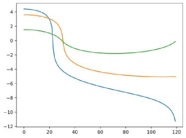
Finally, we calculated the Gaussian curvature for the space of triangles w.r.t to the same four Riemannian metrics: while the Gaussian curvature for the Kendall metric is constant, this is clearly not the case for discrete Sobolev metrics of the present article, cf. Figure 5. Indeed all of the gm{g}^{m} metrics exhibit negative curvature near the points corresponding to triangles with double-points (which do not correspond to elements of d×n\mathbb{R}^{d\times n}_{*}), but only for higher order metrics is this negative curvature strong enough to prevent all geodesics from leaving the space in finite time. More generally, an increase in order leads for a more curved space both for negatively curved regions but also for positively curved regions. Finally, in Figure 6, we further visualize the curvature along selected paths to further demonstrate the behavior at key points of interest. One can see again the increase in negative curvature near the punctures of the sphere.

Refer to caption
Figure 5: The Gaussian curvatures of the space of triangles triangles under the Kendall metric and the discretized scale invariant Sobolev metric gm{g}^{m} for m=0,1,2m=0,1,2). From left to right we have gm{g}^{m} for m=0,1,m=0,1, and 22 and the Kendall metric (with the triangles drawn in). The scale is a symmetric log scale given by sign(x)log(|x+sign(x)|)\operatorname{sign}(x)\log(|x+\operatorname{sign}(x)|).
Refer to caption
Refer to caption
Refer to caption
Refer to caption
Figure 6: These images show the gmg^{m} Gaussian curvatures at each point along the above Kendall geodesics in the space of triangles. The left panel corresponds to the top path and the right panel corresponds with the lower path. Note we omit the Kendall curvature as that would be a constant function 1\equiv 1 on either graph. The curvatures displayed with a symmetric log scale with green corresponding to m=0m=0, orange corresponding to m=1m=1, and blue corresponding to m=2m=2.

Appendix A Constant Coefficient Sobolev Metrics

Our use of the (c)\ell(c) terms in Gm{G}^{m} metrics allowed for scale invariance. These terms may be removed to arrive at the constant coefficient Sobolev metrics

G~cm(h,k):=S1h,k+Dsmh,Dsmkds.\widetilde{G}_{c}^{m}(h,k):=\int_{S^{1}}\langle h,k\rangle+\langle D_{s}^{m}h,D_{s}^{m}k\rangle ds.

These lack scale invariance, but the manifolds (Imm(S1,d),G~m)(\operatorname{Imm}(S^{1},\mathbb{R}^{d}),\widetilde{G}^{m}) are otherwise similar to the scale invariant formulation with identical completeness properties [8, 14, 15]. We can likewise drop the (c)\ell(c) terms from our discretized metrics to arrive at constant coefficient discrete metrics g~m\widetilde{g}^{m}. These also converge to the corresponding smooth G~m\widetilde{G}^{m} like the scale invariant formulation, using exactly the same proof as used for Proposition 1, but without the (c)\ell(c) terms in FF. Similarly, the parallel of the completeness statement, Theorem 2 still holds. The removal of the length terms does not impact the proofs of cases 1 or 2 beyond changing the relevant MM, but the proof for case 3 no longer works. We make use of the following lemma for an alternative proof, stated here in a much more narrow and simple context than in its original form.

Lemma 7 ( Lemma 3.2 in [14]).

Let (,g)(\mathcal{M},g) be a Riemannian manifold with a weakly continuous metric and f:f:\mathcal{M}\to\mathbb{R} a C1C^{1}-function. Assume that for each metric ball B(y,r)B(y,r) in \mathcal{M} there exists a constant CC, such that

|dfdh|C(1+|f(x)|)hg\left|\frac{df}{dh}\right|\leq C(1+|f(x)|)\|h\|_{g}

holds for all xB(y,r)x\in B(y,r) and all hTxh\in T_{x}\mathcal{M}. Then the function

f:(M,d)(,||)f:(M,d)\to(\mathbb{R},|\cdot|)

is continuous and Lipschitz continuous on every metric ball. In particular, ff is bounded on every metric ball.

With this we can re-prove case 3 for the constant coefficient case.

Proof.

Note that it is sufficient to show that 1(c)\frac{1}{\ell(c)} and (c)\ell(c) are bounded on every metric ball to handle case 3. By the above lemma then, it is sufficient to show that

|d(1/(c))dh|C(1+|1/(c)|)hg~2\left|\frac{d(1/\ell(c))}{dh}\right|\leq C(1+|1/\ell(c)|)\|h\|_{\widetilde{g}^{2}}

We do this directly.

|ddh1(c)|=1(c)2ddhi=1n|ei|=1(c)2i=1nhi+1hi,ei|ei|1(c)2i=1nhi+1hi|ei|ei|ei|\left|\frac{d}{dh}\frac{1}{\ell(c)}\right|=\frac{1}{\ell(c)^{2}}\frac{d}{dh}\sum_{i=1}^{n}|e_{i}|=\frac{1}{\ell(c)^{2}}\sum_{i=1}^{n}\frac{\langle h_{i+1}-h_{i},e_{i}\rangle}{|e_{i}|}\leq\frac{1}{\ell(c)^{2}}\sum_{i=1}^{n}\frac{\|h_{i+1}-h_{i}\|}{\sqrt{|e_{i}|}}\frac{\|e_{i}\|}{\sqrt{|e_{i}|}}
1(c)2(i=1nhi+1hi2|ei|)12(i=1n|ei|)12=1(c)32(i=1nhi+1hi2|ei|)121(c)32g~c2(h,h)\leq\frac{1}{\ell(c)^{2}}\left(\sum_{i=1}^{n}\frac{\|h_{i+1}-h_{i}\|^{2}}{|e_{i}|}\right)^{\frac{1}{2}}\left(\sum_{i=1}^{n}|e_{i}|\right)^{\frac{1}{2}}=\frac{1}{\ell(c)^{\frac{3}{2}}}\left(\sum_{i=1}^{n}\frac{\|h_{i+1}-h_{i}\|^{2}}{|e_{i}|}\right)^{\frac{1}{2}}\leq\frac{1}{\ell(c)^{\frac{3}{2}}}\sqrt{\widetilde{g}^{2}_{c}(h,h)}

So that at any particular cc the constant C=(c)C=\sqrt{\ell(c)} yields the desired inequality. We can show via similar work that (c)\sqrt{\ell(c)} is globally Lipschitz:

|ddh(c)|1(c)(i=1nhi+1hi2|ei|)12(i=1n|ei|)12=(i=1nhi+1hi2|ei|)12g~c2(h,h).\left|\frac{d}{dh}\sqrt{\ell(c)}\right|\leq\frac{1}{\sqrt{\ell(c)}}\left(\sum_{i=1}^{n}\frac{\|h_{i+1}-h_{i}\|^{2}}{|e_{i}|}\right)^{\frac{1}{2}}\left(\sum_{i=1}^{n}|e_{i}|\right)^{\frac{1}{2}}=\left(\sum_{i=1}^{n}\frac{\|h_{i+1}-h_{i}\|^{2}}{|e_{i}|}\right)^{\frac{1}{2}}\leq\sqrt{\widetilde{g}^{2}_{c}(h,h)}.

Thus we can indeed choose a CC for any metric ball as needed for the lemma for 1(c)\frac{1}{\ell(c)}. Thus 1(c)\frac{1}{\ell(c)} and (c)\ell(c) are bounded on all metric balls and therefore no path γ:[0,1)d×n\gamma:[0,1)\to\mathbb{R}^{d\times n}_{*} such that limt1γ(t)=0\lim_{t\to 1}\gamma(t)=0 or \infty can be of finite length. ∎

The item most complicated by the removal of the length terms is the relation between g~˙cm(h,h)\dot{\widetilde{g}}^{m}_{c}(h,h) and g~˙cm+1(h,h)\dot{\widetilde{g}}^{m+1}_{c}(h,h). As g˙cm=g~˙cm(c)3+2m\dot{{g}}^{m}_{c}=\dot{\widetilde{g}}^{m}_{c}\cdot\ell(c)^{-3+2m} the statement of Lemma 4 here becomes

g~˙cm(h,h)(c)24g~˙cm+1(h,h)\dot{\widetilde{g}}^{m}_{c}(h,h)\leq\frac{\ell(c)^{2}}{4}\dot{\widetilde{g}}^{m+1}_{c}(h,h)

which is a parallel to the equivalent statement for the smooth constant coefficient case as seen in the proof of Lemma 2.13 of [15].

Appendix B Approximating derivatives in LL^{\infty}

Lemma 8.

Let ff be a bounded function in C(S1)C^{\infty}(S^{1}). Let θi=in\theta_{i}=\frac{i}{n} and define

In0:C(S1)L(S1)I_{n}^{0}:C^{\infty}(S^{1})\to L^{\infty}(S^{1})

so that In0(f)=g0I_{n}^{0}(f)=g_{0} where g0g_{0} is the piecewise constant function where g0(θ)=f(θi)g_{0}(\theta)=f(\theta_{i}) for θ[θi,θi+1)\theta\in[\theta_{i},\theta_{i+1}). Further define In1(f)=g1I_{n}^{1}(f)=g_{1} where g1(θ)=n(f(θi+1)f(θi))g_{1}(\theta)=n(f(\theta_{i+1})-f(\theta_{i})) for θ[θi,θi+1)\theta\in[\theta_{i},\theta_{i+1}). Then

limnIn0(f)fL=0andlimnIn1(f)fL=0.\lim_{n\to\infty}\|I_{n}^{0}(f)-f\|_{L^{\infty}}=0\qquad\text{and}\qquad\lim_{n\to\infty}\|I_{n}^{1}(f)-f^{\prime}\|_{L^{\infty}}=0.
Proof.

Note that S1S^{1} is compact so that our smooth, bounded function ff is Lipschitz continuous. Now if KK is our Lipschitz constant then 0supθ[θi,θi+1)|g0(θ)f(θ)|Kn0\leq\sup_{\theta\in[\theta_{i},\theta_{i+1})}|g_{0}(\theta)-f(\theta)|\leq\frac{K}{n} but this does not depend on ii. This means that as nn\to\infty this supremum goes to 0 and thus also

limng(θ)f(θ)L=limnmaxi=1,,nesssupθ[θi,θi+1)(g0(θ)f(θ))=0.\lim_{n\to\infty}\|g(\theta)-f(\theta)\|_{L^{\infty}}=\lim_{n\to\infty}\max_{i=1,\ldots,n}\operatorname{esssup}_{\theta\in[\theta_{i},\theta_{i+1})}\left(g_{0}(\theta)-f(\theta)\right)=0.

For the second operator we choose nn Lipschitz constants, one for each ii with Ki=supθ[θi,θi+1)f(θ)K_{i}=\sup_{\theta\in[\theta_{i},\theta_{i+1})}f^{\prime}(\theta) being the constant we will use for [θi,θi+1)[\theta_{i},\theta_{i+1}). This means supf(θi+1)f(θi)Kin\sup f(\theta_{i+1})-f(\theta_{i})\leq\frac{K_{i}}{n}. We note immediately as nn\to\infty Kif(θi)K_{i}\to f^{\prime}(\theta_{i}) since ff is smooth. Leaning on this fact makes the work swift:

In1(f)fL\displaystyle\|I_{n}^{1}(f)-f^{\prime}\|_{L^{\infty}} =g(θ)f(θ)L=maxi=1,,nn(f(θi+1)f(θi))fL\displaystyle=\|g(\theta)-f^{\prime}(\theta)\|_{L^{\infty}}=\max_{i=1,\ldots,n}\|n\cdot(f(\theta_{i+1})-f(\theta_{i}))-f^{\prime}\|_{L^{\infty}} (4)
maxi=1,,nn(Kin)fL=maxi=1,,nKifL0 as n\displaystyle\leq\max_{i=1,\ldots,n}\|n\cdot(\frac{K_{i}}{n})-f^{\prime}\|_{L^{\infty}}=\max_{i=1,\ldots,n}\|K_{i}-f^{\prime}\|_{L^{\infty}}\to 0\text{ as }n\to\infty (5)

Define I~n1(f)\widetilde{I}_{n}^{1}(f) analogously to In1(f)I_{n}^{1}(f), but with g1(θ)=n(f(θi)f(θi1))g_{1}(\theta)=n\cdot(f(\theta_{i})-f(\theta_{i-1})) for θ[θi,θi+1)\theta\in[\theta_{i},\theta_{i+1}) and note that this is also such that limnI~n1(f)fL=0\lim_{n\to\infty}\|\widetilde{I}_{n}^{1}(f)-f^{\prime}\|_{L^{\infty}}=0.

Appendix C Proof of Lemma 4

Before we are able to present the proof of Lemma 4 we will need an additional technical Lemma:

Lemma 9.

Let m1m\geq 1, let cd×nc\in\mathbb{R}^{d\times n}_{*} and hTcd×nd×nh\in T_{c}\mathbb{R}^{d\times n}_{*}\cong\mathbb{R}^{d\times n}, we then have

maxk/n|Dsm1(hk+1)Dsm1(hk)|ek||12i=1n|Dsm1(hi+1)Dsm1(hi)|ei|Dsm1(hi)Dsm1(hi1)|ei1||\max_{k\in\mathbb{Z}/n\mathbb{Z}}\left|\frac{D_{s}^{m-1}(h_{k+1})-D_{s}^{m-1}(h_{k})}{|e_{k}|}\right|\leq\frac{1}{2}\sum_{i=1}^{n}\left|\frac{D_{s}^{m-1}(h_{i+1})-D_{s}^{m-1}(h_{i})}{|e_{i}|}-\frac{D_{s}^{m-1}(h_{i})-D_{s}^{m-1}(h_{i-1})}{|e_{i-1}|}\right| (6)

for odd mm and

maxk/n|Dsm1(hk)Dsm1(hk1)μk|12i=1n|Dsm1(hi+1)Dsm1(hi)μi+1Dsm1(hi)Dsm1(hi1)μi|\max_{k\in\mathbb{Z}/n\mathbb{Z}}\left|\frac{D_{s}^{m-1}(h_{k})-D_{s}^{m-1}(h_{k-1})}{\mu_{k}}\right|\leq\frac{1}{2}\sum_{i=1}^{n}\left|\frac{D_{s}^{m-1}(h_{i+1})-D_{s}^{m-1}(h_{i})}{\mu_{i+1}}-\frac{D_{s}^{m-1}(h_{i})-D_{s}^{m-1}(h_{i-1})}{\mu_{i}}\right| (7)

for even mm.

Proof.

This Lemma follows by direct estimation. Therefore, let k/nk\in\mathbb{Z}/n\mathbb{Z} and note that j=1n(Ds(hj+1)Ds(hj))=0\sum_{j=1}^{n}(D_{s}(h_{j+1})-D_{s}(h_{j}))=0 as each term appears in the sum both in positive form and negative. Then, for odd mm,

|Dsm1(hk+1)Dsm1(hk)|ek||\displaystyle\left|\frac{D_{s}^{m-1}(h_{k+1})-D_{s}^{m-1}(h_{k})}{|e_{k}|}\right|
=|1(c)j=1n(Dsm1(hj+1)Dsm1(hj))Dsm1(hk+1)Dsm1(hk)|ek||\displaystyle=\left|\frac{1}{\ell(c)}\sum_{j=1}^{n}(D_{s}^{m-1}(h_{j+1})-D_{s}^{m-1}(h_{j}))-\frac{D_{s}^{m-1}(h_{k+1})-D_{s}^{m-1}(h_{k})}{|e_{k}|}\right|
=|1(c)j=1n(Dsm1(hj+1)Dsm1(hj))1(c)j=1nDsm1(hk+1)Dsm1(hk)|ek||ej||\displaystyle=\left|\frac{1}{\ell(c)}\sum_{j=1}^{n}(D_{s}^{m-1}(h_{j+1})-D_{s}^{m-1}(h_{j}))-\frac{1}{\ell(c)}\sum_{j=1}^{n}\frac{D_{s}^{m-1}(h_{k+1})-D_{s}^{m-1}(h_{k})}{|e_{k}|}|e_{j}|\right|
|1(c)j=1n(Dsm1(hj+1)Dsm1(hj)|ej|Dsm1(hk+1)Dsm1(hk)|ek|)|ej||\displaystyle\leq\left|\frac{1}{\ell(c)}\sum_{j=1}^{n}\left(\frac{D_{s}^{m-1}(h_{j+1})-D_{s}^{m-1}(h_{j})}{|e_{j}|}-\frac{D_{s}^{m-1}(h_{k+1})-D_{s}^{m-1}(h_{k})}{|e_{k}|}\right)|e_{j}|\right|
|1(c)j=1n12(i=kj1(Dsm1(hi+i)Dsm1(hi)|ei|Dsm1(hi)Dsm1(hi1)|ei1|)\displaystyle\leq\left|\frac{1}{\ell(c)}\sum_{j=1}^{n}\frac{1}{2}\left(\sum_{i=k}^{j-1}\left(\frac{D_{s}^{m-1}(h_{i+i})-D_{s}^{m-1}(h_{i})}{|e_{i}|}-\frac{D_{s}^{m-1}(h_{i})-D_{s}^{m-1}(h_{i-1})}{|e_{i-1}|}\right)\right.\right.
i=jk1(Dsm1(hi+1)Dsm1(hi)|ei|Dsm1(hi)Dsm1(hi1)|ei1|))|ej||\displaystyle\left.\left.\qquad\qquad\qquad-\sum_{i=j}^{k-1}\left(\frac{D_{s}^{m-1}(h_{i+1})-D_{s}^{m-1}(h_{i})}{|e_{i}|}-\frac{D_{s}^{m-1}(h_{i})-D_{s}^{m-1}(h_{i-1})}{|e_{i-1}|}\right)\right)|e_{j}|\right|
12(c)j=1ni=1n|Dsm1(hi+1)Dsm1(hi)|ei|Dsm1(hi)Dsm1(hi1)|ei1|||ej|\displaystyle\leq\frac{1}{2\ell(c)}\sum_{j=1}^{n}\sum_{i=1}^{n}\left|\frac{D_{s}^{m-1}(h_{i+1})-D_{s}^{m-1}(h_{i})}{|e_{i}|}-\frac{D_{s}^{m-1}(h_{i})-D_{s}^{m-1}(h_{i-1})}{|e_{i-1}|}\right||e_{j}|
12i=1n|Dsm1(hi+1)Dsm1(hi)|ei|Dsm1(hi)Dsm1(hi1)|ei1||\displaystyle\leq\frac{1}{2}\sum_{i=1}^{n}\left|\frac{D_{s}^{m-1}(h_{i+1})-D_{s}^{m-1}(h_{i})}{|e_{i}|}-\frac{D_{s}^{m-1}(h_{i})-D_{s}^{m-1}(h_{i-1})}{|e_{i-1}|}\right|

The case for even mm is similar, swapping |ei||e_{i}| for μi\mu_{i} and rotating some indices.

|Dsm1(hk)Dsm1(hk1)μk|\displaystyle\left|\frac{D_{s}^{m-1}(h_{k})-D_{s}^{m-1}(h_{k-1})}{\mu_{k}}\right|
=|1(c)j=1n(Dsm1(hj)Dsm1(hj1))Dsm1(hk)Dsm1(hk1)μk|\displaystyle=\left|\frac{1}{\ell(c)}\sum_{j=1}^{n}(D_{s}^{m-1}(h_{j})-D_{s}^{m-1}(h_{j-1}))-\frac{D_{s}^{m-1}(h_{k})-D_{s}^{m-1}(h_{k-1})}{\mu_{k}}\right|
=|1(c)j=1n(Dsm1(hj)Dsm1(hj1))1(c)j=1nDsm1(hk)Dsm1(hk1)μkμj|\displaystyle=\left|\frac{1}{\ell(c)}\sum_{j=1}^{n}(D_{s}^{m-1}(h_{j})-D_{s}^{m-1}(h_{j-1}))-\frac{1}{\ell(c)}\sum_{j=1}^{n}\frac{D_{s}^{m-1}(h_{k})-D_{s}^{m-1}(h_{k-1})}{\mu_{k}}\mu_{j}\right|
|1(c)j=1n(Dsm1(hj)Dsm1(hj1)μjDsm1(hk)Dsm1(hk1)μk)μj|\displaystyle\leq\left|\frac{1}{\ell(c)}\sum_{j=1}^{n}\left(\frac{D_{s}^{m-1}(h_{j})-D_{s}^{m-1}(h_{j-1})}{\mu_{j}}-\frac{D_{s}^{m-1}(h_{k})-D_{s}^{m-1}(h_{k-1})}{\mu_{k}}\right)\mu_{j}\right|
|1(c)j=1n12(i=kj1(Dsm1(hi+i)Dsm1(hi)μi+1Dsm1(hi)Dsm1(hi1)μi)\displaystyle\leq\left|\frac{1}{\ell(c)}\sum_{j=1}^{n}\frac{1}{2}\left(\sum_{i=k}^{j-1}\left(\frac{D_{s}^{m-1}(h_{i+i})-D_{s}^{m-1}(h_{i})}{\mu_{i+1}}-\frac{D_{s}^{m-1}(h_{i})-D_{s}^{m-1}(h_{i-1})}{\mu_{i}}\right)\right.\right.
i=jk1(Dsm1(hi+1)Dsm1(hi)μi+1Dsm1(hi)Dsm1(hi1)μi))μj|\displaystyle\left.\left.\qquad\qquad\qquad-\sum_{i=j}^{k-1}\left(\frac{D_{s}^{m-1}(h_{i+1})-D_{s}^{m-1}(h_{i})}{\mu_{i+1}}-\frac{D_{s}^{m-1}(h_{i})-D_{s}^{m-1}(h_{i-1})}{\mu_{i}}\right)\right)\mu_{j}\right|
12(c)j=1ni=1n|Dsm1(hi+1)Dsm1(hi)μiDsm1(hi)Dsm1(hi1)μi1|μj\displaystyle\leq\frac{1}{2\ell(c)}\sum_{j=1}^{n}\sum_{i=1}^{n}\left|\frac{D_{s}^{m-1}(h_{i+1})-D_{s}^{m-1}(h_{i})}{\mu_{i}}-\frac{D_{s}^{m-1}(h_{i})-D_{s}^{m-1}(h_{i-1})}{\mu_{i-1}}\right|\mu_{j}
12i=1n|Dsm1(hi+1)Dsm1(hi)μi+1Dsm1(hi)Dsm1(hi1)μi|\displaystyle\leq\frac{1}{2}\sum_{i=1}^{n}\left|\frac{D_{s}^{m-1}(h_{i+1})-D_{s}^{m-1}(h_{i})}{\mu_{i+1}}-\frac{D_{s}^{m-1}(h_{i})-D_{s}^{m-1}(h_{i-1})}{\mu_{i}}\right|

This proves the lemma. ∎

Proof of Lemma 4.

We consider the odd case which is not meaningfully different from the even one. Following from Lemma 9, we have

maxi/n|Dm1(hk+1)Dm1(hk)|ek||2\displaystyle\max_{i\in\mathbb{Z}/n\mathbb{Z}}\left|\frac{D^{m-1}(h_{k+1})-D^{m-1}(h_{k})}{|e_{k}|}\right|^{2}
14(i=1n|Dsm1hi+1Dsm1(hi)|ei|Dsm1(hi)Dsm1(hi1)|ei1||)2\displaystyle\leq\frac{1}{4}\left(\sum_{i=1}^{n}\left|\frac{D_{s}^{m-1}h_{i+1}-D_{s}^{m-1}(h_{i})}{|e_{i}|}-\frac{D_{s}^{m-1}(h_{i})-D_{s}^{m-1}(h_{i-1})}{|e_{i-1}|}\right|\right)^{2}
14(i=1n|Dsm1(hi+1)Dsm1(hi)|ei|Dsm1(hi)Dsm1(hi1)|ei1||21μi)(i=1nμi)\displaystyle\leq\frac{1}{4}\left(\sum_{i=1}^{n}\left|\frac{D_{s}^{m-1}(h_{i+1})-D_{s}^{m-1}(h_{i})}{|e_{i}|}-\frac{D_{s}^{m-1}(h_{i})-D_{s}^{m-1}(h_{i-1})}{|e_{i-1}|}\right|^{2}\frac{1}{\mu_{i}}\right)\left(\sum_{i=1}^{n}\mu_{i}\right)
=(c)4(i=1n|Dsm1(hi+1)Dsm1(hi)|ei|Dsm1(hi)Dsm1(hi1)|ei1||21μi).\displaystyle=\frac{\ell(c)}{4}\left(\sum_{i=1}^{n}\left|\frac{D_{s}^{m-1}(h_{i+1})-D_{s}^{m-1}(h_{i})}{|e_{i}|}-\frac{D_{s}^{m-1}(h_{i})-D_{s}^{m-1}(h_{i-1})}{|e_{i-1}|}\right|^{2}\frac{1}{\mu_{i}}\right).

Then, due to Hölder’s inequality and the above, we conclude

g˙cm(h,h)\displaystyle\dot{{g}}_{c}^{m}(h,h) =i=1n(c)3+2m|Dsm(hi)|2|ei|\displaystyle=\sum_{i=1}^{n}\ell(c)^{-3+2m}|D_{s}^{m}(h_{i})|^{2}|e_{i}|
=i=1n3+2m|Dsm1(hi+1)Dsm1(hi)|2|ei|\displaystyle=\sum_{i=1}^{n}\ell^{-3+2m}\frac{|D_{s}^{m-1}(h_{i+1})-D_{s}^{m-1}(h_{i})|^{2}}{|e_{i}|}
(c)3+2m(maxk𝒞n|Dsm1(hk+1)Dsm1(hk)|ek||2)(k=1n|ek|)\displaystyle\leq\ell(c)^{-3+2m}\left(\max_{k\in\mathcal{C}_{n}}\left|\frac{D_{s}^{m-1}(h_{k+1})-D_{s}^{m-1}(h_{k})}{|e_{k}|}\right|^{2}\right)\left(\sum_{k=1}^{n}|e_{k}|\right)
(c)3+2m(c)24i=1n|Dsm1(hi+1)Dsm1(hi)|ei|Dsm1(hi)Dsm1(hi1)|ei1||21μi\displaystyle\leq\ell(c)^{-3+2m}\frac{\ell(c)^{2}}{4}\sum_{i=1}^{n}\left|\frac{D_{s}^{m-1}(h_{i+1})-D_{s}^{m-1}(h_{i})}{|e_{i}|}-\frac{D_{s}^{m-1}(h_{i})-D_{s}^{m-1}(h_{i-1})}{|e_{i-1}|}\right|^{2}\frac{1}{\mu_{i}}
=(c)3+2(m+1)4i=1n|Dsm+1(hi)|2μi=14g˙cm+1(h,h).\displaystyle=\frac{\ell(c)^{-3+2(m+1)}}{4}\sum_{i=1}^{n}|D_{s}^{m+1}(h_{i})|^{2}\mu_{i}=\frac{1}{4}\dot{{g}}_{c}^{m+1}(h,h).

This is symmetric with the argument for the odd case, which we omit. ∎

References

  • [1] C. J. Atkin. The hopf-rinow theorem is false in infinite dimensions. Bulletin of the London Mathematical Society, 7(3):261–266, 1975.
  • [2] C. J. Atkin. Geodesic and metric completeness in infinite dimensions. Hokkaido Mathematical Journal, 26(1):1–61, 1997.
  • [3] M. Bauer, M. Bruveris, P. Harms, and P. W. Michor. Vanishing geodesic distance for the riemannian metric with geodesic equation the kdv-equation. Annals of Global Analysis and Geometry, 41:461–472, 2012.
  • [4] M. Bauer, M. Bruveris, P. Harms, and P. W. Michor. Soliton solutions for the elastic metric on spaces of curves. Discrete and Continuous Dynamical Systems, 38(3):1161–1185, 2018.
  • [5] M. Bauer, M. Bruveris, P. Harms, and J. Møller-Andersen. A Numerical Framework for Sobolev Metrics on the Space of Curves. SIAM Journal on Imaging Sciences, 10(1):47–73, 2017.
  • [6] M. Bauer, M. Bruveris, and B. Kolev. Fractional sobolev metrics on spaces of immersed curves. Calculus of Variations and Partial Differential Equations, 57:1–24, 2018.
  • [7] M. Bauer, M. Bruveris, and P. W. Michor. Overview of the Geometries of Shape Spaces and Diffeomorphism Groups. Journal of Mathematical Imaging and Vision, 50(1):60–97, 2014.
  • [8] M. Bauer and P. Harms. Metrics on spaces of immersions where horizontality equals normality. Differential Geometry and its Applications, 39:166–183, 2015.
  • [9] M. Bauer, P. Harms, and S. C. Preston. Vanishing distance phenomena and the geometric approach to sqg. Archive for Rational Mechanics and Analysis, 235(3):1445–1466, 2020.
  • [10] M. Bauer, P. Heslin, and C. Maor. Completeness and geodesic distance properties for fractional sobolev metrics on spaces of immersed curves. The Journal of Geometric Analysis, 34(7):214, 2024.
  • [11] M. Bauer, C. Maor, and P. Michor. Sobolev metrics on spaces of manifold valued curves. Annali Scuola Normale Superiore-Classe di Scienze, page 47–47, 2022.
  • [12] J. Bernal, G. Dogan, and C. R. Hagwood. Fast dynamic programming for elastic registration of curves. In Proceedings of the IEEE Conference on Computer Vision and Pattern Recognition Workshops, page 111–118, 2016.
  • [13] S. Beutler, F. Hartwig, M. Rumpf, and B. Wirth. Discrete geodesic calculus in the space of sobolev curves. In preparation, 2024.
  • [14] M. Bruveris. Completeness properties of sobolev metrics on the space of curves. Journal of Geometric Mechanics, 7(2):125–150, 2015.
  • [15] M. Bruveris, P. W. Michor, and D. Mumford. Geodesic Completeness for Sobolev Metrics on the Space of Immersed Plane Curves. In Forum of Mathematics, Sigma, volume 2. Cambridge University Press, 2014.
  • [16] M. Bruveris and F.-X. Vialard. On completeness of groups of diffeomorphisms. Journal of the European Mathematical Society, 19(5):1507–1544, 2017.
  • [17] E. Celledoni, S. Eidnes, and A. Schmeding. Shape analysis on homogeneous spaces: a generalised srvt framework. In Computation and Combinatorics in Dynamics, Stochastics and Control: The Abel Symposium, Rosendal, Norway, August 2016, page 187–220. Springer, 2018.
  • [18] K. Crane. Discrete differential geometry: An applied introduction. Notices of the AMS, Communication, 1153, 2018.
  • [19] K. Crane, F. De Goes, M. Desbrun, and P. Schröder. Digital geometry processing with discrete exterior calculus. In ACM SIGGRAPH 2013 Courses, page 1–126. 2013.
  • [20] I. Ekeland. The hopf-rinow theorem in infinite dimension. Journal of Differential Geometry, 13(2):287–301, 1978.
  • [21] K. Habermann, P. Harms, and S. Sommer. Long-time existence of brownian motion on configurations of two landmarks. Bulletin of the London Mathematical Society, 56(5):1658–1679, 2024.
  • [22] D. G. Kendall. Shape manifolds, Procrustean metrics, and complex projective spaces. Bull. London Math. Soc, 16:81–121, 1984.
  • [23] S. Lang. Differential manifolds, volume 2. Springer, 1972.
  • [24] P. W. Michor and D. Mumford. Vanishing Geodesic Distance on Spaces of Submanifolds and Diffeomorphisms. Documenta Mathematica, 10:217–245, 2005.
  • [25] P. W. Michor and D. Mumford. An Overview of the Riemannian Metrics on Spaces of Curves Using the Hamiltonian Approach. Applied and Computational Harmonic Analysis, 23(1):74–113, 2007.
  • [26] D. B. Mumford and P. W. Michor. Riemannian geometries on spaces of plane curves. Journal of the European Mathematical Society, 8(1):1–48, 2006.
  • [27] T. Needham and S. Kurtek. Simplifying Transforms for General Elastic Metrics on the Space of Plane Curves. SIAM journal on imaging sciences, 13(1):445–473, 2020.
  • [28] X. Pennec, S. Sommer, and T. Fletcher. Riemannian Geometric Statistics in Medical Image Analysis. Academic Press, 2019.
  • [29] A. Srivastava, E. Klassen, S. H. Joshi, and I. H. Jermyn. Shape Analysis of Elastic Curves in Euclidean Spaces. IEEE Transactions on Pattern Analysis and Machine Intelligence, 33(7):1415–1428, 2010.
  • [30] A. Srivastava and E. P. Klassen. Functional and Shape Data Analysis, volume 1. Springer, 2016.
  • [31] G. Sundaramoorthi, A. Yezzi, and A. C. Mennucci. Sobolev active contours. International Journal of Computer Vision, 73:345–366, 2007.
  • [32] L. Younes. Shapes and Diffeomorphisms, volume 171. Springer, 2010.