Sobolev Inequalities in Spacelike Submanifolds of Minkowski Space
Abstract.
We follow the method of ABP estimate in [Bre21] and apply it to spacelike submanifolds in . We then obtain Michael-Simon type inequalities. Surprisingly, our investigation leads to a Sobolev inequality without a mean curvature term, provided the hypersurface is mean convex.
1. Introduction
In this paper we are mainly concerned with a specific type of Sobolev inequality for spacelike submanifolds in Minkowski space. Associated to a spacelike submanifold , we define the maximal slope by
See 2.1 for details. The main results are as follows.
Theorem 1.1.
Suppose is a smooth, compact and spacelike hypersurface. Assume that is mean convex and that is any smooth and positive function defined on . Then
| (1.1) |
where the constant .
Under the condition of mean convexity, there is no mean curvature term involved, which, to our knowledge, is new, Without the assumption of mean convexity, similar result holds with a curvature term involved.
Theorem 1.2.
Suppose is a smooth, compact and spacelike hypersurface. Assume that is any smooth and positive function defined on . Then
| (1.2) |
with .
Here ; see Section 2 for details. Next we establish the same Sobolev inequality for submanifold of higher codimension , with . Let be a normal vector field of with . We then write , where . Accordingly, the mean curvature vector is decomposed into .
Theorem 1.3.
Suppose is a smooth, compact and spacelike submanifold. Let be any normal vector field of with and any smooth and positive function defined on . Then
| (1.3) |
where the constant .
At the end of this work, we discovered that in [TW22] similar results were established. Nevertheless, compared to the results therein, our construction yields a Sobolev inequality without curvature terms for a mean convex hypersurface. The history of geometric inequalities probably dates back to ancient Greece. The classical isoperimetric inequality asserts that for a domain with sufficiently well-behaved boundary, there holds
| (1.4) |
It is known that such an isoperimetric inequality is essentially equivalent to the Sobolev inequality for domains in Euclidean space:
| (1.5) |
Intensive work has been established to extend Eq. 1.4 or Eq. 1.5 to more general settings. It has long been conjectured that the same inequality Eq. 1.4 holds in Cartan-Hadamard manifolds [Aub76]. Partial results include [Wei26, BR33, Cro84, Kle92]. See also [GS21] for a recent attempt to resolve the conjecture. It is also possible to replace areas and volumes in Eq. 1.4 by more general quermassintegrals. The resulting isoperimetric inequality is proved for hypersurfaces with certain convexity in Euclidean space. See [Gua] for details.
For a domain in a two dimensional space form of constant curvature , there is a neat result which states that
| (1.6) |
Please see [Cho05] and references therein. The same inequality Eq. 1.6 is proved by Choe and Gulliver [CG92a] for minimal surfaces with certain topological constraints in hyperbolic space . Yau [Yau75], Choe and Gulliver [CG92] showed that if is a domain in or a -dimensional minimal submanifold in , then it satisfies the linear isoperimetric inequality
Another linear inequality for proper minimal submanifolds in is obtained in [MS14] using Poincaré model.
It is a longstanding conjecture that Eq. 1.4 holds true for minimal hypersurfaces in . Using the method of sliding, Brendle fully settled the problem in a recent work [Bre21], and later extended his results to Riemannian manifolds with nonnegative Ricci curvature [Bre20]. The most classical application of the sliding method is perhaps Aleksandrov’s maximum principle. In [Cab08] Cabré first employed the sliding method and gave a simple and elegant proof of Eq. 1.4.
We follow Brendle’s method and apply it to submanifolds in the Minkowski space, and obtain some Michael-Simon-Sobolev type inequalities.
Acknowledgements. The author would like to thank Research Professor Qi-Rui Li for his instructions and many helpful discussions.
2. Notations and Preliminaries
Let be the Minkowski space endowed with metric
The usual Euclidean metric of is denoted by . The volume element of , , is just the usual Lebesgue measure. A vector is called unit if , where is the signature of , i.e. if is spacelike, timelike, lightlike, respectively. Finally, we define .
Let be a spacelike hypersuface. We denote by a point in , and by the corresponding position vector in . Anything with a ‘bar’ is a quantity of the ambient space. Then the second fundamental form is defined by
Let be a normal to at the point . Clearly is also a vector in . Denote by the -th coordinate of in , so that
Definition 2.1.
Associated to a spacelike submanifold , the maximal slope is defined by
The quantity characterizes how ‘lightlike’ is; for instance, if ; and is uniquely determined by the diameter if .
Lemma 2.2.
For any function on the ambient space, .
Proof.
We assume that is spanned by orthonormal basis , and by , with . We then compute
By Gauss formula we see that and . Hence
By tensorality, the same formula holds in any coordinate systems. ∎
3. Proof of 1.1
Since Eq. 1.1 is homogeneous in , by normalization we may assume that
| (3.1) |
Let be the outward unit normal of . Consider the following PDE
| (3.2) |
By our normalization, the equation has a solution . Since is mean convex, we may assume that the mean curvature vector is either zero or timelike pointing to the past. Let be the unit normal and timelike vector field pointing to the past. Now fix . For any we define , where
| (3.3) |
Note that when , the notation simply means the normal .
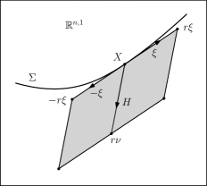
We write , where is a unit tangent vector and is a unit normal vector pointing to the past. The the definition of implies that . Therefore is a parallelogram illustrated as in Fig. 1. We continue and define
Finally, we take the map ,
| (3.4) |
Lemma 3.1.
We have asymptotic behavior
| (3.5) |
where is the usual Lebesgue measure in and .
Proof.
We blow down by factor . As , the bounded domain collapses to a single point: the origin, and each converges to a , specified by
where is the unit normal to at pointing to the past. See the left of Fig. 2 for an illustration. Clearly contains the cone .
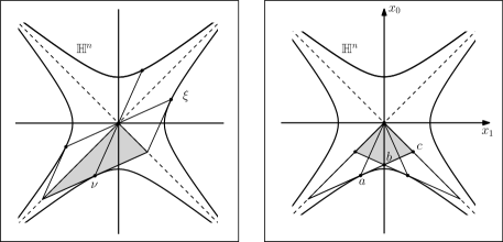
Therefore contains at least . Since by assumption has minimal height , we may assume that is the union of two cones, as illustrated by the right of Fig. 2, with the zeroth coordinate of point being .
We now proceed by computing the volume of . Without loss of generality, we assume that the points lie in the plane . Then , and the tengential is parallel to . From this we readily obtain and . Consequently
Hence . ∎
Lemma 3.2.
There holds .
Proof.
For any given , consider the function
By compactness attains its minimum at some . We claim that . For if otherwise , then at this point We have by definition of that , a contradiction. Hence and at which . We then find such that . Obviously and . Finally, by 2.2,
completing the proof. ∎
In the Riemannian or Lorentzian setting, in order for the area formula to be true, the Jacobian of a map should be modified with volume elements; that is,
where is the usual tangent map of the coordinate map.
Lemma 3.3.
The invariant Jacobian of is given by
Proof.
At a fixed point , we pick an orthonormal basis that spans , and a normal coordinate system such that at . Then . We now compute
Note that we have used the fact that and that . Thus , whence
By tensorality the same formula holds in any coordinate system. ∎
Lemma 3.4.
We have for any
Proof.
By definition, for any . Therefore
On the other hand, from Eq. 3.2 and the fact that , we have
completing the proof. ∎
4. Proof of 1.2
Without the ‘mean convexity’ assumption, the union , with defined by Eq. 3.3, might as well be empty. We therefore construct by
| (4.1) |
Since Eq. 1.2 is homogeneous in , we may assume
| (4.2) |
so that Eq. 4.1 admits a solution. We then modify Eq. 3.3 by
and . Accordingly,
and . Note that when , the notation simply means the normal vector . Similar as in Section 3, we still have
-
•
The inclusion ; and
-
•
The Jacobian .
The proofs are almost identical.
Lemma 4.1.
We have asymptotic behavior
| (4.3) |
where .
Proof.

Lemma 4.2.
We have for any
Proof.
By definition, for any . Therefore
Moreover, we have
Combined with Eq. 4.1, it follows that
giving the assertion. ∎
5. Proof of 1.3
We fix such a section , with ; that is, is a unit timelike normal vector field along . At each point , we have decompostion
where . Note that is a spacelike subspace. Accordingly, we write a normal vector as . The equation we consider now is
| (5.1) |
We normalize by
| (5.2) |
so that the PDE has a solution. The domains and codomains are
Finally we take . As in Section 3,
-
•
The inclusion ; and
-
•
The Jacobian .
The proofs are almost identical.
Lemma 5.1.
We have asymptotic behavior
| (5.3) |
where .
Proof.
Lemma 5.2.
We have for any
Proof.
By geometric-arithmetic inequality,
Now by Eq. 5.1, we have
On the other hand, by the definition of ,
This implies that , completing the proof. ∎
References
- [Aub76] Thierry Aubin “Problèmes Isopérimétriques et Espaces de Sobolev” In Journal of Differential Geometry 11.4, 1976, pp. 573–598 DOI: 10.4310/jdg/1214433725
- [BR33] E. F. Beckenbach and T. Rado “Subharmonic Functions and Surfaces of Negative Curvature” In Transactions of the American Mathematical Society 35.3, 1933, pp. 662 DOI: 10.2307/1989854
- [Bre20] Simon Brendle “Sobolev Inequalities in Manifolds with Nonnegative Curvature”, 2020, pp. 1–25 arXiv: http://arxiv.org/abs/2009.13717
- [Bre21] Simon Brendle “The Isoperimetric Inequality for a Minimal Submanifold in Euclidean Space” In Journal of the American Mathematical Society 34.2, 2021, pp. 595–603
- [CG92] Jaigyoung Choe and Robert Gulliver “Isoperimetric Inequalities on Minimal Submanifolds of Space Forms” In Manuscripta Mathematica 77, 1992, pp. 169–189
- [CG92a] Jaigyoung Choe and Robert Gulliver “The Sharp Isoperimetric Inequality for Minimal Surfaces with Radially Connected Boundary in Hyperbolic Space” In Inventiones Mathematicae 109.1, 1992, pp. 495–503 DOI: 10.1007/BF01232035
- [Cab08] Xavier Cabré “Elliptic PDE’s in Probability and Geometry: Symmetry and Regularity of Solutions” In Discrete and Continuous Dynamical Systems 20.3, 2008, pp. 425–457 DOI: 10.3934/dcds.2008.20.425
- [Cho05] Jaigyoung Choe “Isoperimetric Inequalities of Minimal Submanifolds” In Global theory of minimal surfaces, 2005, pp. 325–370
- [Cro84] Christopher B. Croke “A Sharp Four Dimensional Isoperimetric Inequality” In Commentarii Mathematici Helvetici 59.1, 1984, pp. 187–192 DOI: 10.1007/BF02566344
- [GS21] Mohammad Ghomi and Joel Spruck “Total Curvature and the Isoperimetric Inequality in Cartan-Hadamard Manifolds” arXiv, 2021 arXiv: http://arxiv.org/abs/1908.09814
- [Gua] Pengfei Guan “Curvature Measures, Isoperimetric Type Inequalities and Fully Nonlinear Pdes”
- [Kle92] Bruce Kleiner “An Isoperimetric Comparison Theorem” In Inventiones Mathematicae 108.1, 1992, pp. 37–47 DOI: 10.1007/BF02100598
- [MS14] Sung Hong Min and Keomkyo Seo “Optimal Isoperimetric Inequalities for Complete Proper Minimal Submanifolds in Hyperbolic Space” In Journal fur die Reine und Angewandte Mathematik, 2014, pp. 203–214 DOI: 10.1515/crelle-2012-0119
- [TW22] Chung-Jun Tsai and Kai-Hsiang Wang “An Isoperimetric-Type Inequality for Spacelike Submanifold in the Minkowski Space” In International Mathematics Research Notices 2022.1, 2022, pp. 128–139 DOI: 10.1093/imrn/rnaa084
- [Wei26] André Weil “Sur Les Surfaces a Courbure Negative” In CR Acad. Sci. Paris 182.2, 1926, pp. 1069–1071
- [Yau75] Shing-Tung Yau “Isoperimetric Constants and the First Eigenvalue of a Compact Riemannian Manifold” In Annales scientifiques de l’École normale supérieure 8.4, 1975, pp. 487–507 DOI: 10.24033/asens.1299