Smooth orbit equivalence rigidity for dissipative geodesic flows
Abstract.
Let be a smooth closed orientable surface. A Gaussian thermostat on can be seen as the geodesic flow of a certain metric connection with torsion. These flows may not preserve any smooth volume form. We prove that if two Gaussian thermostats on with negative thermostat curvature are related by a smooth orbit equivalence isotopic to the identity, then the two background metrics are conformally equivalent via a smooth diffeomorphism of isotopic to the identity. We also give a relationship between the thermostat forms themselves. Finally, we prove the same result for Anosov magnetic flows.
1. Introduction
Let be a smooth closed oriented Riemannian surface, and let be a smooth function on the unit tangent bundle . We concern ourselves with the dynamical system governed by the equation
where is the complex structure on induced by the orientation.
This equation defines a flow on which reduces to the geodesic flow when . The flow models the motion of a particle under the influence of a force orthogonal to the velocity and with magnitude . Its generating vector field is , where is the geodesic vector field on , and is the vertical vector field. The system is called a (generalized) thermostat.
If does not depend on the velocity, i.e., if it corresponds to a function on , then is the magnetic flow associated with the magnetic field , where is the area form of . When depends linearly on the velocity, i.e., when it corresponds to a -form on , we instead obtain a Gaussian thermostat, which is reversible in the sense that the flip on conjugates with (just as in the case of geodesic flows). The resulting flows are interesting from a dynamical point of view because, contrary to geodesic or magnetic flows, they may not preserve any smooth volume form (see [DP07]). Gaussian thermostats also appear in geometry as the geodesic flows of certain metric connections with torsion (see [PW08]). We thus think of them as dissipative geodesic flows.
We are interested in rigidity results for generalized thermostats satisfying the Anosov property. By [Ghy84, Theorem A], these flows are topologically orbit equivalent to the geodesic flow of any metric of constant negative curvature on via a Hölder homeomorphism which is in fact isotopic to the identity. In particular, this tells us that the flows of generalized thermostats are transitive and topologically mixing, so the idea is that the richness of the chaotic orbits should allow one to recover information about the system.
The set up is as follows. Given two generalized thermostats and on the same surface , we assume there is a smooth orbit equivalence which is isotopic to the identity. Here is the unit tangent bundle with respect to the metric on , and orbit equivalence means that oriented orbits are mapped to oriented orbits, i.e., there exists such that . In particular, is a conjugacy if is identically . There is a natural identification of with by scaling the fibers via the map
| (1.1) |
By saying that is isotopic to the identity we mean that is isotopic to the identity in the usual sense.
Question: If both thermostat flows are Anosov, what is the relationship, if any, between and ?
The work in [GLP24] gives an answer in the case where and is a conjugacy. The metrics and must be isometric via an isometry isotopic to the identity. Instead of starting with a smooth conjugacy isotopic to the identity, they start with the equivalent assumption that both metrics have the same marked length spectrum. The two assumptions are also equivalent for magnetic flows, but having the same marked length spectra only guarantees a Hölder continuous conjugacy in general.
Still with as a conjugacy, the paper [Gro99] deals with the mixed case where is a magnetic system and is geodesic, but at the cost of additional assumptions: has negative Gaussian curvature, has the same area with respect to and , and neither nor its first derivative are too big. The conclusion is then that and are isometric via an isometry isotopic to the identity and that .
More recently, progress has been made with [Reb23] to understand a deformative version of our question in the purely magnetic case, framed through the lens of marked length spectrum rigidity.
1.1. Main results
Beyond its physical motivation, the magnetic case represents the first step towards the broader goal of understanding generalized thermostats: it corresponds to the case where has Fourier degree (see §2.1.4). Our first main result is the following:
Theorem 1.1.
Let and be two Anosov magnetic systems on a smooth closed orientable surface . If there is a smooth orbit equivalence isotopic to the identity between them, then there exists a smooth diffeomorphism , isotopic to the identity, such that for some . Moreover, if the orbit equivalence is a conjugacy and , then if and only if .
We note that finding a relationship between and in the general magnetic case remains an open question. A key similarity between geodesic and magnetic flows is that they preserve the Liouville measure on . As we will explain, this allows most of the key arguments from the paper [GLP24] to also go through in the magnetic case.
For this reason, the main emphasis of this paper is instead on Gaussian thermostats. These correspond to the case where or, equivalently,
| (1.2) |
for some 1-form on , where denotes the restriction to of smooth differential forms (so that we may see them as functions on ). We will denote a Gaussian thermostat by to highlight its particular form.
One can also study Gaussian thermostats using an external vector field . This is the vector field on characterized by , that is, the vector field dual to , where is the Hodge star operator of the metric (given by oriented rotation by in the case of -forms).
As we allow to have Fourier degree 1, we introduce the possibility of new dynamical features absent from the geodesic and magnetic cases. For instance, by [DP07, Theorem A], a Gaussian thermostat preserves an absolutely continuous invariant measure on if and only if is exact. This means that the Liouville measure may no longer be preserved, and it allows for fractal SRB measures.
The thermostat curvature of is the quantity
| (1.3) |
where is the Gaussian curvature of . If , then the flow is Anosov by [Woj00, Theorem 5.2], in analogy with the geodesic case. Note that equation (1.3) is a particular case of the more general definition
| (1.4) |
used for any generalized thermostat .
This leads us to our next main result.
Theorem 1.2.
Let and be two Gaussian thermostats with on a smooth closed orientable surface . If there is a smooth orbit equivalence isotopic to the identity between them, then there exists a smooth diffeomorphism , isotopic to the identity, such that for some . Moreover, if either or is closed, then is exact.
As shown in Lemma 4.6, the scaling map defined in (1.1) yields a smooth orbit equivalence isotopic to the identity between the Gaussian thermostats and , with a time-change by . This implies that the conformal factor in our main result is optimal and that it is necessary to leave room for an exact difference when relating the -forms. However, it is unclear at this stage whether the closedness condition is really necessary to establish this last relationship.
Ideally, one would like to extend this result to the general Anosov case. The only place where we use the negative thermostat curvature is in showing that the Gaussian thermostats satisfy the attenuated tensor tomography problem of order (see §2.3.2). We do not have this issue in the purely magnetic case, which is why we were able to simply assume the more general Anosov property in Theorem 1.1. Removing the negative thermostat curvature assumption should also allow one to mix the magnetic case with Gaussian thermostats, i.e., to take .
As pointed out above, there are still open questions regarding the rigidity of for of Fourier degree . It is also unclear at this stage how much information is gained from having a genuine conjugacy versus an orbit equivalence, and whether the conjugating diffeomorphism itself must have some particular form as in the purely geodesic case (see [GLP24, Corollary 1.2]).
After this work, a natural question is whether anything can be said for of Fourier degree . As we show with the no-go Lemma 2.16, the current argument does not work for these thermostats. However, there are interesting examples of such systems. For instance, when is the real part of a holomorphic differential of degree , the corresponding thermostat admits an interpretation as coupled vortex equations (see [MP19]). It was also shown in [MP20] that the geodesic flow of an affine connection on is, up to a time-change, the flow of a generalized thermostat with of the form . Just as we have shown that a non-trivial Anosov magnetic system cannot be smoothly conjugate to an Anosov geodesic flow by a conjugacy isotopic to the identity, it would be interesting to further categorize generalized thermostats.
Finally, we note that Theorem A.5, which applies to generalized thermostats, was placed in the appendix to improve the overall exposition of the paper, but it represents a new result related to the injectivity of the generalized thermostat X-ray transform.
1.2. Strategy
Our main inspiration is the approach in [GLP24]. Indeed, we show that a smooth orbit equivalence isotopic to the identity determines the complex structure of the metric up to biholomorphisms isotopic to the identity (Proposition 4.2). This allows us to conclude that the two metrics and must be conformally equivalent via a smooth diffeomorphism of isotopic to the identity.
To show that the orbit equivalence determines the complex structure, we rely on Torelli’s theorem (Theorem 2.8), which tells us that it is enough to show that the period matrix of the underlying Riemann surface is preserved. To be able to conclude that the resulting diffeomorphism is isotopic to the identity, we use the fact that the argument can be repeated on any finite cover.
The period matrix is defined in terms of holomorphic -forms on . We show with Theorem 2.15 that these can always be associated to the first Fourier modes of certain distributions on satisfying a transport equation and with non-negative Fourier modes (see §2.2.2). Asking for these distributions to only have non-negative Fourier modes is a critical requirement for the rest of the argument, but it does not carry over to the case of generalized thermostats when has Fourier degree .
We then establish in Lemma 3.6 a pairing formula showing that the integral of any holomorphic -form over a thermostat geodesic on (i.e., the periods of the period matrix) is the same as the integral over of an associated -current invariant by and living in a certain subspace (see §2.1.3). This pairing formula then tells us that the smooth orbit equivalence preserves the period matrix.
At a high level, there are two main challenges and departures from [GLP24]: the first is in handling a general orbit equivalence instead of a conjugacy, and the second is in dealing with the fact that Gaussian thermostats may not be volume-preserving.
The presence of a non-zero divergence with respect to the Liouville form manifests itself in a few ways. First, instead of flow-invariant distributions, the right object of study becomes solutions to the dual transport equation. This subspace is no longer preserved by the pullback of the orbit equivalence, so we have to introduce the space of -currents mentioned above and establish a one-to-one relationship with the distributions solving the transport equation (Lemma 2.3). We then have to check that the wavefront set analysis is unaffected by factoring the correspondence through this space (Lemma 2.4) and that is mapped to (Proposition 3.3).
Another complication due to the dissipation is in showing that any holomorphic 1-form can be seen as the first Fourier mode of an element in , as previously mentioned. The heavy lifting to address this issue is done in Appendix A. Furthermore, again due to the divergence, we have to explain why Gaussian thermostats with negative thermostat curvature satisfy the attenuated tensor tomography problem of order 1 (Theorem 2.12).
For the pairing formula previously described, we have replaced the role of the Liouville form with that of a certain form defined in (2.2). Finally, to relate with , we rely on new arguments which at their core involve the smooth Livšic theorem.
1.3. Organization of the paper
In Section 2, we introduce the background tools necessary for the rest of the paper. Specifically, §2.1 provides a short introduction to the geometry and Fourier analysis of the unit tangent bundle. It also introduces the new objects needed to deal with the divergence of the generalized thermostats. In §2.2, we review the complex geometry and harmonic analysis on a surface, while §2.3 delves into hyperbolic dynamics and tensor tomography.
In Section 3, we explain how a smooth orbit equivalence acts on holomorphic differentials, and we establish the pairing formula needed to show that period matrices are preserved. We then present the proofs of our main results in Section 4.
Appendix A delves into the question of finding distributional solutions, with prescribed Fourier modes, of the relevant transport equation for a generalized thermostat.
Acknowledgements
I would like to thank my advisor, Gabriel Paternain, for suggesting this project and guiding me while working on it.
2. Preliminaries
In what follows, is a smooth closed oriented Riemannian surface, and we take an arbitrary . Whenever we use additional assumptions, it will be clearly stated in the result statements. We will sometimes need a second generalized thermostat . All the objects depending on the metric will then be labeled accordingly. Finally, we denote by a smooth orbit equivalence between the thermostats and . Once again, we will specify when we assume it to be isotopic to the identity.
2.1. Unit tangent bundle of the surface
We review some basics of the unit tangent bundle defined by
2.1.1. Geometry of
As previously, let be the geodesic vector field on , and let be the vertical vector field generating the circle action on the fibers. We define . The vector fields form an orthonormal basis on for the Sasaki metric (the natural lift of to ). We set and . We also note that the geodesic vector field splits into where are the raising and lowering Guillemin-Kazhdan operators given by
| (2.1) |
The Liouville -form is defined by and . It is invariant by the geodesic flow in the sense that . The -form is non-degenerate on the contact plane , and it satisfies . Hence
is a volume form invariant by the geodesic flow. We call it the Liouville volume form. It corresponds to the Riemannian volume form induced by the Sasaki metric on . From now on, the space on is defined as .
We also define the -forms on by and . It is easy to check that so that . We set , , , and . We refer to [PSU23, Chapter 3] for further details on the geometric structure on .
2.1.2. Appearance of the divergence
The key difference between generalized thermostats and geodesic or magnetic flows is that the generating vector field might not preserve the Liouville volume form . Recall that the divergence of the vector field with respect to the volume form is the function uniquely defined by
The following result is proved in [DP07, Lemma 3.2].
Lemma 2.1.
Let be a generalized thermostat. Then, we have:
In the geodesic and magnetic cases, we have , so the Liouville volume form is preserved. Another way in which the divergence manifests itself is when calculating the adjoint operators with respect to the inner product on :
This is relevant when extending differential operators to act on the space of distributions. Recall that any differential operator with smooth real-valued coefficients acts on a distribution by duality, that is for any . The subspace of distributional solutions to the transport equation
thus corresponds to the distributions such that for all . If , these are simply the distributions invariant by the flow.
2.1.3. Divergence and smooth orbit equivalences
It will prove important to understand how the divergence of a system interacts with smooth orbit equivalences.
The next result, which we have stated in a broader setting than the one we are studying in this paper to highlight its generality, relates the divergences of two flows associated by a smooth orbit equivalence.
Lemma 2.2.
Let and be two orientable manifolds endowed with nowhere-vanishing volume forms and , and smooth vector fields and . Suppose is a smooth orbit equivalence between the flows generated by and . If we write with and with , then
In particular, if preserves the orientation, i.e., , then
Proof.
We compute
On the other hand, we also have
so putting these together yields the desired result since is nowhere-vanishing. ∎
In the geodesic and magnetic cases, the pullback of the smooth orbit equivalence sends the space to . More generally, however, the divergence term appearing in the transport equation breaks this down.
Instead, a more useful perspective is to look at the following subspace of -currents (or distributional -forms) on invariant by :
This set only depends on the foliation corresponding to , i.e., it is invariant under time-changes, so we get a -linear isomorphism . The 2-form
| (2.2) |
then allows us to establish a relationship with solutions to the transport equation.
Lemma 2.3.
The map given by is a -linear isomorphism.
Proof.
Using Cartan’s magic formula and Lemma 2.1, note that
Therefore, is closed if and only if . Since never vanishes, any -current on satisfying must be of the form for some . ∎
Thanks to this identification, we can now define a map associated to the smooth orbit equivalence via the following diagram:
| (2.3) |
This point of view does not affect the wavefront set analysis.
Lemma 2.4.
If preserves the orientation, then, for all , we have
Proof.
Let be the function such that . Then, we get
Since multiplication by the nowhere-vanishing function is elliptic, we get the result by elliptic regularity (see [Hö03, Theorem 8.3.2]).
∎
By the properties of wavefront sets under pullback operators (see [Hö03, Theorem 8.2.4] for instance), we thus obtain
for all , where is the symplectic lift of to the cotangent bundles given by
2.1.4. Fourier decomposition
The space breaks up as
This decomposition is orthogonal with respect to the inner product on and with being replaced by . For any , we shall write , where each is given by
| (2.4) |
with being the flow generated by . More generally, any distribution can be decomposed as , where each is defined by
and satisfies .
If a distribution on only has finitely many non-trivial Fourier modes, we say that it has finite Fourier degree. The smallest such that for all is then called the Fourier degree of .
It also worth noting that the ladder operators in (2.1) take their name from the fact that they act as raising/lowering operators on the Fourier decomposition, that is,
for all . In particular, we have for any .
2.2. Complex geometry
The conformal class of the Riemannian metric and the orientation of induce a complex structure on , making it into a Riemann surface which we denote by .
2.2.1. Complex structures.
The Teichmüller space of , denoted by , is the space of complex structures on modulo the equivalence relation that if and only if there exists a diffeomorphism , isotopic to the identity, such that . We will denote such an equivalence class of complex structures by .
The mapping class group is defined as the quotient of orientation preserving diffeomorphisms on modulo isotopy. They act on by pullback, and the quotient space is the moduli space of complex structures on . See [FM11] for a thorough introduction.
Each complex structure determines a canonical line bundle on . We will denote by the space of -holomorphic sections of the -th tensor power of the canonical line bundle . Locally, its elements have the form for and for .
2.2.2. Fiberwise holomorphic distributions
Each subspace of Fourier modes can be identified with , the set of smooth sections of the bundle . Indeed, we have a -linear isomorphism
given by restriction to , i.e., in local coordinates (for ),
This is a generalization of the map which we have already encountered in (1.2) to identify smooth -forms with . Note that the definition of depends on the choice of the metric . We denote by its -adjoint. In local coordinates, we have
Once we extend the operators to distributions by duality, the projection onto the -th Fourier mode is simply given by acting on .
Under this identification, we can essentially think of the raising/lowering operators as and operators thanks to the following result (see [PSU14, Lemma 2.1] and the ensuing discussion).
Lemma 2.5.
For , the following diagram commutes:
For , the operator also intertwines the operators and .
As a result, for , the operator gives us an identification
We also introduce the following terminology:
Definition 2.6.
A distribution is said to be fiberwise holomorphic if for all .
Equivalently, if we define the Szegö projectors by
then a distribution is fiberwise holomorphic if and only if . The projectors satisfy the commutation relations
| (2.5) |
We will be interested in the family of fiberwise holomorphic distributions that satisfy the transport equation:
| (2.6) |
2.2.3. Torelli’s theorem
The complex vector space of -holomorphic -forms has the same dimension as the genus of (see [FK92, Proposition III.2.7]). Given a canonical basis of the homology on , the following result gives us the existence of a useful basis (see [FK92, Proposition, p. 63]).
Proposition 2.7.
There exists a unique basis for with the property
| (2.7) |
Furthermore, the matrix with -entry
is symmetric with positive definite imaginary part.
The space of symmetric matrices with positive definite imaginary part and size given by the genus of is called the Siegel upper half-space . We thus get a well-defined period matrix map
The following form of Torelli’s theorem tells us that period matrices capture a lot of the information about the complex structure.
Theorem 2.8.
Assume that has genus . If , then there exists an orientation-preserving diffeomorphism such that .
We refer to [FK92, Theorem III.12.3] for a proof.
2.3. Hyperbolic dynamics
We now further assume that the flow of the generalized thermostat is Anosov (or uniformly hyperbolic).
2.3.1. Definition
Recall that the Anosov property means that there exists a flow-invariant continuous splitting
and uniform constants and such that for all we have
| (2.8) |
In the geodesic case, the contact form is preserved, so . It is then known that . For a generalized thermostat, we instead know by [DP07, Lemma 4.1] that
| (2.9) |
Here are the weak stable and unstable bundles. This implies that there exist such that
| (2.10) |
In fact, the weak stable and unstable bundles are (see [Has94, Corollary 1.8]), so the functions are also (and smooth along the flow since each bundle is -invariant). The Anosov property implies that everywhere. One may in fact show that , so the basis is positively-oriented.
Lemma 2.9.
Let be an Anosov generalized thermostat. Then, the functions uniquely characterized by (2.10) satisfy .
Proof.
Since everywhere, it suffices to show the inequality at a single point. By compactness, we can pick such that . Let us define
Differentiating with respect to and setting , we obtain
Using that yields
Since , there exists a unique constant such that belongs to . Therefore, given that and are uniformly attracting and repelling sets on respectively, we must have at this point.
∎
Remark 2.10.
Note that, when and , i.e., in the geodesic case with negative curvature, we have the stronger statement because .
The dual bundles are defined by
One can check we have similar estimates to (2.8) for and , with replaced by (inverse transpose). Translated to the setting of the cotangent bundle, property (2.9) then becomes
| (2.11) |
Further note that
where
is the characteristic set of the operator (usually defined without the zero section).
2.3.2. Tensor tomography
The tensor tomography problem is interesting in its own right, particularly as it pertains to the injectivity of the X-ray transform for thermostats. We will need the following property in the case .
Definition 2.11.
We say that a thermostat satisfies the attenuated tensor tomography problem of order if having with and of Fourier degree implies that is of Fourier degree .
The term ‘attenuated’ refers to the presence of the divergence in the transport equation. Note that such a term appears for Gaussian thermostats and generalized thermostats of higher Fourier degree, but not for magnetic or geodesic flows.
The fact that geodesic flows satisfy the (attenuated) tensor tomography problem was first proved in negative curvature in [GK80] for and then generalized to the Anosov case in [DS03] for , [PSU14] for , and [Gui17] for . It was also shown in [DP05] that Anosov magnetic flows satisfy the (attenuated) tensor tomography problem of order .
For generalized thermostats of higher Fourier degree, the non-attenuated and attenuated versions of the tensor tomography problem are different. In [DP07], it was proved that Gaussian thermostats (potentially mixed with a magnetic component) satisfy the non-attenuated tensor tomography problem of order . We instead need:
Theorem 2.12.
Any Gaussian thermostat with satisfies the attenuated tensor tomography problem of order .
This result is a consequence of the work in [AR21]. Their argument heavily relies on the negative thermostat curvature assumption. In particular, most of the heavy lifting is done by [AR21, Theorem 3.1], where the Carleman estimates for Gaussian thermostats with negative curvature are established (akin to the work in [PS23]):
Theorem 2.13.
Let be a Gaussian thermostat with for some . For any integer and parameter , we have
for all .
The rest of the argument is then relatively straightforward for our case, which is less general than the one tackled in [AR21]. We include it here for the sake of completeness, but also to show how it can be simplified.
Proposition 2.14.
Let be a Gaussian thermostat with . Suppose has finite Fourier degree and satisfies . Then also has finite Fourier degree.
Proof.
We follow the argument from [AR21, Theorem 5.1]. Let be the Fourier degree of . Since , we obtain
As a result, there exists such that
Pick such that , fix , and let . We can apply Theorem 2.13 to get
Since , we note that
so that
It hence follows that
However, we have by design, so for all .
∎
Proof of Theorem 2.12.
Finally, the proofs of our theorems rely on the possibility of lifting arbitrary holomorphic -forms to solutions of the transport equation. As explained in Appendix A, where we have relegated most of the work on this front, this is again related to the injectivity of the X-ray transform for thermostats.
Theorem 2.15.
Let , with of Fourier degree , be an Anosov thermostat. For any holomorphic (resp. anti-holomorphic) -form on , there exists with for all (resp. ) such that and (resp. ).
Proof.
Let us treat the case where the -form is holomorphic. The anti-holomorphic case is completely analogous. Using Lemma 2.5, we know that is in the kernel of . We can hence apply Theorem A.5, which tells us that there exists with such that and . We project this distribution onto its positive Fourier components to get . For all , we then have
which entails that . ∎
We note that we cannot hope to get such a result for an arbitrary .
Lemma 2.16.
Suppose where and . Since has isolated zeroes, there exists with and . Then, there is no with for all such that and .
Proof.
Suppose such a distribution exists. For any , we must have
Therefore, applying this to , we get , a contradiction.∎
3. Action on holomorphic differentials
We have seen that, by passing through a specific type of -currents instead of directly using the pullback , the linear map defined in (2.3) sends distributional solutions to the transport equation of one generalized thermostat to those of the second. In this section, we want to show that can also be seen as acting on holomorphic differentials from one complex surface to another when is of Fourier degree and the attenuated tensor tomography problem of order is satisfied.
3.1. Action on fiberwise holomorphic distributions
We start by studying the action of on the subspace defined in (2.6). This will require some microlocal analysis.
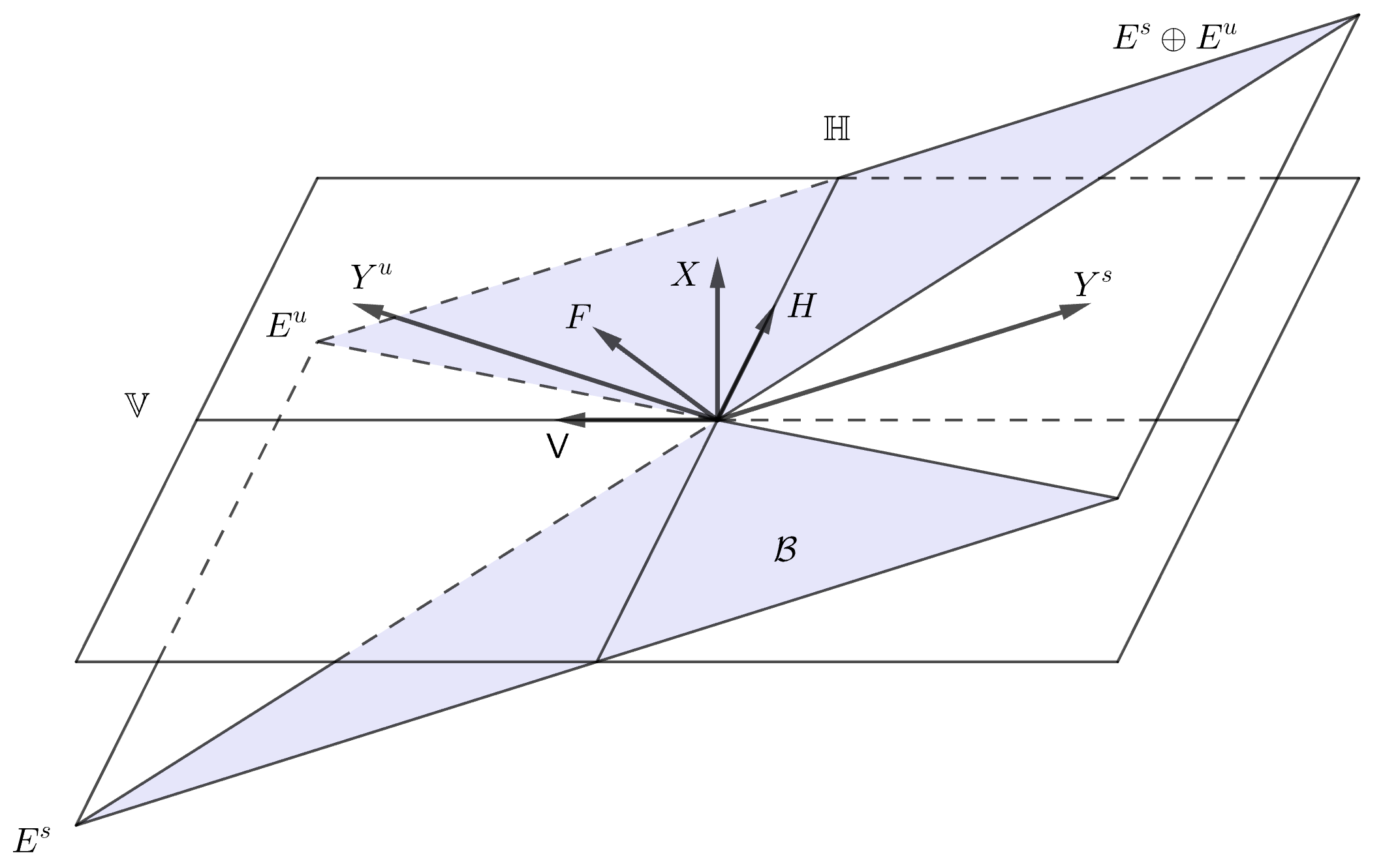
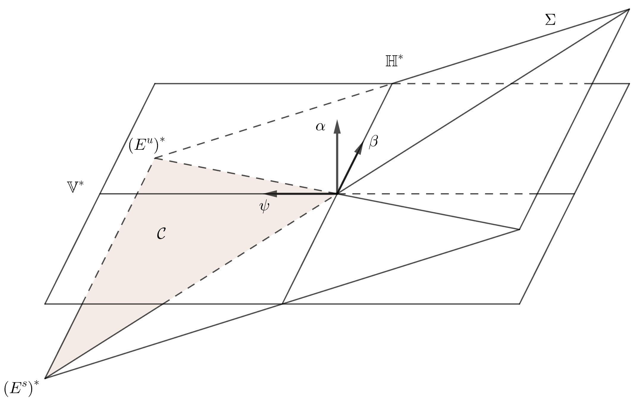
We introduce , the closed cone enclosed by and in the half-space . See Figure 1.
Lemma 3.1.
Let be an Anosov generalized thermostat. If , then and for all .
Proof.
The argument is essentially the same as that of [GLP24, Lemma 2.5]. Let us give the details.
By definition, each satisfies . Using the wavefront set description of the Schwartz kernel of (see [Gui17, Lemma 3.10]), we thus get
Given that , elliptic regularity tells us that
By propagation of singularities for real principal type differential operators (see [Hö09, Theorem 26.1.1]), we further know that is invariant by the symplectic lift of the flow . Given the Anosov property, the maximal flow-invariant subset of contained in is , so this gives us the first claim.
For the second claim, recall that . The pushforward operator only selects the wavefront set in (see [FT99, Proposition 11.3.3]), which is empty given that by property (2.11). Therefore .
∎
We will also need the following lemma with the same proof as [GLP24, Lemma 3.3].
Lemma 3.2.
Let and be Anosov generalized thermostats. Suppose there exists a smooth orbit equivalence isotopic to the identity between them. Then preserves the natural orientation of the weak unstable bundle, namely that given by the basis .
Armed with this, we can show that maps fiberwise holomorphic distributional solutions to the transport equation of one thermostat to those of the second. For this step of the proof, however, we restrict to thermostats where has Fourier degree and the attenuated tensor tomography problem of order is satisfied.
Proposition 3.3.
Let and , with and of Fourier degree , be Anosov thermostats satisfying the attenuated tensor tomography problem of order . Suppose there exists a smooth orbit equivalence isotopic to the identity between them. Then the map defined in (2.3) yields a -linear isomorphism
Proof.
Since maps connected sets to connected sets, to , and to , must be one of the four cones depicted on the right of Figure 1 (inside the characteristic set ). It follows that because any other cone would entail that reverses the orientation, which is impossible since it is assumed to be isotopic to the identity. If , then would flip the orientation of the weak unstable leaves, which contradicts Lemma 3.2. Therefore .
Let and . By Lemma 3.1, we know that . By Lemma 2.4, we thus know that . Then and, since , we also have that
Since satisfies the tensor tomography problem of order by assumption, it follows that is of Fourier degree . Hence is fiberwise holomorphic. The fact that is an isomorphism is then clear as it admits an inverse, namely the map associated to by (2.3). ∎
3.2. Extension operator
Next, we show how can be seen as acting on holomorphic differentials from one complex surface to another. Let us start by noting that the map
| (3.1) |
is well-defined. Indeed, if , then , which means that and hence . By Lemma 2.5, this is equivalent to .
3.3. Period preservation
The following result shows that the induced mapping of holomorphic differentials we have just defined preserves additional structure.
Proposition 3.4.
Let and , with and of Fourier degree , be Anosov thermostats satisfying the attenuated tensor tomography problem of order . The -linear map
is an isomorphism. It preserves periods in the sense that, for all and , we have
Recall that there is a push-forward map given by integration along fibers. It satisfies (see [BT82, Proposition 6.14]), and it extends to currents. By [BT82, Proposition 6.15], we have the projection formula
| (3.3) |
for any smooth oriented curve on and any 2-form on .
Lemma 3.5.
Let be a generalized thermostat. For any , we have
Proof.
It suffices to establish the claim for . Recall that . A quick computation then yields
| (3.4) |
Note that , where is the area form on .
Pick and take . Then, by definition, we have
where is a lift of under . We take , i.e., no component in the subbundle . Then, since , we get
Given that , we obtain
where in the last equality we used the formula (2.4). In terms of -forms, since , we proved that
We conclude by applying to both sides.
∎
We can then integrate this identity, applied to solutions of the transport equation, over closed thermostat geodesics to obtain the following result.
Lemma 3.6.
Let be an Anosov generalized thermostat and a closed thermostat geodesic. For any , the pairing is well-defined and
Proof.
By the wavefront set calculus, the pairing is well-defined whenever
| (3.5) |
(see [Hö03, Corollary 8.2.7] for instance). The conormal bundle consists of a line contained in , so Lemma 3.1 and property (2.11) tell us that the intersection with is indeed empty. It follows that the pairing is well-defined and extends the pairing computed for .
We can then apply the projection formula (3.3) and Lemma 3.5. As seen in Lemma 2.3, the -current is closed if , so is also closed given that , which implies that its integral only depends on the homology class .
∎
As , for any we may write
Therefore, if , , and is any thermostat geodesic whose homology class is , Lemma 3.6 gives us
| (3.6) |
We can now tackle the proof of Proposition 3.4.
Proof of Proposition 3.4.
Let and let , be two thermostat geodesics (with respect to and ) whose homology class is . Since is isotopic to the identity, we know that in .
We claim that the pairing is well-defined. The tangent space to is . By property (2.9), it trivially intersects the closed cone enclosed by and , and whose orthogonal projection onto avoids . Since preserves the orientation, the same arguments as in Proposition 3.3 tell us that the tangent space to intersects the closed cone trivially. As a result, its conormal avoids the closed cone , which contains by Lemma 3.1. The wavefront set condition (3.5) is hence satisfied.
The -current is closed by Lemma 2.3. By the Hodge decomposition theorem, we may hence write for some harmonic -current and -current with . Thanks to the wavefront set condition, the same argument as for then shows that both pairings and are well-defined. They must be equal to since is exact. We thus get
where in the second equality we have used the fact that is harmonic and in .
We can now use (3.6) and unravel the definitions to obtain
∎
4. End of the proofs
4.1. Torelli’s theorem
The work from the previous section, when combined with Torelli’s theorem, tells us that a smooth orbit equivalence isotopic to the identity determines the class in the moduli space of complex structures on .
Proposition 4.1.
Let and , with and of Fourier degree , be Anosov thermostats satisfying the attenuated tensor tomography problem of order . If there exists a smooth orbit equivalence isotopic to the identity between them, then in . Equivalently, there exists a diffeomorphism such that and for some .
Proof.
By Proposition 3.4, the map is a period-preserving -linear isomorphism. This means that and have the same period matrix. Indeed, given a canonical basis of the homology on , let be a basis for such that property (2.7) is satisfied. Then is a basis for such that (2.7) is also satisfied, and
Since the surface must be of genus , Theorem 2.8 tells us that there exists an orientation-preserving diffeomorphism such that .
∎
In this section, we want to show something stronger, namely, that the class of the complex structure is determined in Teichmüller space .
Proposition 4.2.
Let and be either
-
(a)
two Anosov magnetic systems, or
-
(b)
two Gaussian thermostats with .
If there exists a smooth orbit equivalence isotopic to the identity between them, then in . Equivalently, there exists a diffeomorphism , isotopic to the identity, such that and for some .
The reason we needed to specify the nature of the two thermostats, as opposed to Proposition 4.1 which deals with more general Anosov thermostats of Fourier degree , is that our proof relies the following technical lemma (see [GLP24, Lemma 3.8]).
Lemma 4.3.
Let and be two complex structures on compatible with orientation such that in . Then, there exists a finite cover such that the lifts are not in the same -orbit.
Indeed, when lifting the thermostats to finite covers, the properties of being Anosov and having negative thermostat curvature are preserved, but, a priori, satisfying the attenuated tensor tomography problem of order is not.
Proof Proposition 4.2.
Suppose, for the sake of contradiction, that in . By Lemma 4.3, there exists a finite cover such that the lifts and are not in the same -orbit.
Since the smooth orbit equivalence between the flows of and is isotopic to the identity, it can be lifted to a smooth orbit equivalence isotopic to the identity between the flows of and .
In case (a), we know that the lifted Anosov magnetic flows on are again Anosov because the cover is finite. They hence satisfy the (attenuated) tensor tomography problem of order . In case (b), we know that the lifted Gaussian thermostats also have negative thermostat curvature since the property is local. By Theorem 2.12, we thus conclude that they satisfy the attenuated tensor tomography problem of order .
We can then apply Proposition 4.1 to obtain a contradiction. ∎
4.2. Rigidity of the magnetic field
Since does not depend on the velocity in the magnetic case, we will think of it as living in .
Lemma 4.4.
Let be an Anosov magnetic flow. Then, the -form on defined in (2.2) is exact.
Proof.
By (3.4), we have
By the Gauss-Bonnet theorem and the fact must be of genus , we know that
so in . It follows that we may write for some -form on and . The constant is explicitly given by
| (4.1) |
But then, since , we obtain
which allows us to write for the 1-form
| (4.2) |
∎
Knowing how to find primitives of in the magnetic case then unlocks the following.
Proposition 4.5.
Let and be two Anosov magnetic systems with the same background metric . Suppose there is a smooth conjugacy , isotopic to the identity, between them. Then, we have in . Moreover, if and only if .
Proof.
Define the as in (4.2) to be a primitive of . Contracting it with yields
| (4.3) |
Moreover, we know that the Anosov magnetic flows are transitive and is isotopic to the identity, so . Since , contracting with yields . This can be rewritten as , which in turn implies
Since is an isomorphism, there exists a closed -form on and such that
Contracting with yields
By (4.3), we thus get
which simplifies to
| (4.4) |
If we integrate with respect to , we obtain (since )
We thus have by (4.1), which shows that the cohomology classes of and in are the same up to a sign.
If , we may take , and we know that thanks to (4.1). It follows that . Let be a closed magnetic geodesic of and . Relation (4.4) allows us to write
By the smooth Livšic theorem [dlLMM86, Theorem 2.1] and [DP05, Theorem B], this means that is exact. Since is closed, we get , which in turn implies , as desired. ∎
We can now conclude the proof of Theorem 1.1.
Proof of Theorem 1.1.
If two Anosov magnetic systems and are related by a smooth conjugacy , isotopic to the identity, Proposition 4.2 yields a diffeomorphism isotopic to the identity such that for some .
If is a conjugacy and , the map gives us a smooth conjugacy isotopic to the identity between the Anosov magnetic flows and . Thus Proposition 4.5 tells us that in and that if and only if .
∎
4.3. Rigidity of the thermostat 1-form
Given the conclusion of Proposition 4.2, it behooves us to understand the behavior of (generalized) thermostat flows under a conformal re-scaling of the metric.
Lemma 4.6.
Let be a generalized thermostat, and define a conformal re-scaling of the metric, for some . Then, the scaling map defined in (1.1), which in this case is simply , satisfies
In particular, the map represents a smooth orbit equivalence isotopic to the identity from to
| (4.5) |
with a time-change .
Proof.
The first statement is proved in [CP22, Lemma B.1]. The conclusion then follows from the calculation
∎
In what follows, let be the -form on satisfying . If is of Fourier degree , we may more succinctly write the thermostat (4.5) as
Proposition 4.7.
Let and , with and of Fourier degree , be two Anosov thermostats. Suppose there is a smooth orbit equivalence , isotopic to the identity, between them. If or is closed, then is exact.
Proof.
By Lemma 2.1, we have , so an application of Lemma 2.2 gives us
where is such that . Therefore, if is a closed thermostat geodesic on with respect to , and , we have
Without loss of generality, suppose that . Then, since is isotopic to the identity and integrals of -forms over curves are independent of the parametrization, we have
Putting these together, we conclude that
An application of the smooth Livšic theorem [dlLMM86, Theorem 2.1] and [DP07, Theorem B] allows us to conclude that is exact, as desired.
∎
We can now conclude the proof of Theorem 1.2.
Proof of Theorem 1.2.
If two Gaussian thermostats and with negative thermostat curvature are related by a smooth orbit equivalence isotopic to the identity, then Proposition 4.2 tells us that there exists a diffeomorphism isotopic to the identity such that for some .
It remains to show that, if either or is closed, then is exact. The map yields a smooth orbit equivalence isotopic to the identity between the Anosov Gaussian thermostats and . By Lemma 4.6, we may assume without loss of generality that . Proposition 4.7 then allows us to conclude.
∎
Appendix A Solutions to the transport equation as extensions
A key ingredient that we use in this paper is Theorem 2.15: it allows us to extend any holomorphic -form on (seen as a function on ) to a fiberwise holomorphic distribution satisfying the transport equation . We say that the distribution is an extension of in the sense that .
This can be seen as part of a larger theme, which is to find distributional solutions of the transport equation with some prescribed Fourier modes. The problem is closely related to the study of the surjectivity of the adjoint of the X-ray transform for thermostats, which in turn is key to understanding the injectivity of the X-ray transform operator itself.
As an example, the following extension result generalizes [Ain15, Theorem 1.6] and [AZ17, Theorem 1.7], which cover the cases of magnetic flows and Gaussian thermostats respectively.
Theorem A.1.
Let be an Anosov generalized thermostat. For any , there exists such that and .
The argument crucially relies on the Pestov identity (see [DP07, Theorem 3.3]).
Theorem A.2.
Let be a generalized thermostat. Then
| (A.1) |
for all .
Recall that the thermostat curvature for a generalized thermostat is defined in (1.4). In both [Ain15] and [AZ17], the proofs introduce the following property:
Definition A.3.
Let . A generalized thermostat is -controlled if
for all .
They then show that magnetic flows and Gaussian thermostats are -controlled for some whenever they are Anosov. However, using the Pestov identity (A.1) for generalized thermostats, the same proof as in [AZ17, Theorem 3.1] goes through for the more general case.
Theorem A.4.
Let be an Anosov generalized thermostat. Then, there exists such that
for all . In particular, is -controlled.
The next theorem is again in the spirit of extending functions with low Fourier degree: it deals with functions induced from 1-forms on . The result requires a technical condition, which is that the smooth -form being considered needs to be solenoidal (or divergence-free) in the sense that . Here is the co-differential with respect to the metric acting on -forms, i.e., . If we write , then if and only if (see [PSU14]).
Theorem A.5.
Let be an Anosov generalized thermostat. For any solenoidal smooth -form on , there exists with such that and .
This is a generalization of [Ain15, Theorem 1.7] and [AZ17, Theorem 1.8], which again deal with the magnetic and Gaussian thermostat cases respectively. However, adapting the proofs requires some care. We will need the following lemma.
Lemma A.6.
For any , the -norms of its Fourier coefficients are rapidly decaying in the sense that, for all , we have
Proof.
For any point on , let be an open neighborhood admitting smooth coordinates such that . The Sobolev embedding theorem gives us a constant such that
for all . Here we use the multi-index notation and define .
Using the explicit formula (2.4) on , we may write
Therefore, still on the domain , we can see that
By compactness, we can cover with a finite number of such open sets . Then, we get
Since the -norms of the Fourier coefficients of a smooth function are rapidly decaying, we obtain the desired result.
∎
The following lemma has the same proof as [AZ17, Theorem 1.8]. The argument relies on the Pestov identity and Theorem A.4.
Lemma A.7.
Let be an Anosov generalized thermostat. Then there exists a constant such that
for all
Next, we define the projection operator by
We also define as .
Lemma A.8.
Let be an Anosov generalized thermostat. Then there exists a constant such that
for all .
Proof.
In this proof, we will let be a constant which can change from line to line to simplify the notation.
By Theorem A.4 and the Pestov identity (A.1), we have
Therefore, we obtain
| (A.2) |
It also gives us
Therefore
and
By the reverse triangle inequality, we get
and
By the triangle inequality, the Cauchy-Schwarz inequality, Lemma A.6, and property (A.2), we obtain
This gives us
The result then follows because
and
∎
References
- [Ain15] Gareth Ainsworth. The magnetic ray transform on Anosov surfaces. Discrete and Continuous Dynamical Systems, 35(5):1801–1816, 2015.
- [AR21] Yernat M. Assylbekov and Franklin T. Rea. The attenuated ray transforms on Gaussian thermostats with negative curvature. arXiv:2102.04571, 2021.
- [AZ17] Yernat M. Assylbekov and Hanming Zhou. Invariant distributions and tensor tomography for Gaussian thermostats. Communications in Analysis and Geometry, 25(5):895–926, 2017.
- [BT82] Raoul Bott and Loring W. Tu. Differential Forms in Algebraic Topology. Springer, 1982.
- [CP22] Mihajlo Cekić and Gabriel P. Paternain. Resonant forms at zero for dissipative Anosov flows. arXiv:2211.06255, 2022.
- [dlLMM86] Rafael de la Llave, José Manuel Marco, and Roberto Moriyón. Canonical perturbation theory of Anosov systems and regularity results for the Livsic cohomology equation. Annals of Mathematics, 123(3):537–611, 1986.
- [DP05] Nurlan S. Dairbekov and Gabriel P. Paternain. Longitudinal KAM-cocycles and action spectra of magnetic flows. Mathematical Research Letters, 12:719–730, 2005.
- [DP07] Nurlan S. Dairbekov and Gabriel P. Paternain. Entropy production in Gaussian thermostats. Communications in Mathematical Physics, 269:533–543, 2007.
- [DS03] Nurlan S. Dairbekov and Vladimir A. Sharafutdinov. Some problems of integral geometry on Anosov manifolds. Ergodic Theory and Dynamical Systems, 23(1):59–74, 2003.
- [FK92] Hershel M. Farkas and Irwin Kra. Riemann Surfaces, volume 71 of Graduate Texts in Mathematics. Springer-Verlag, 2 edition, 1992.
- [FM11] Benson Farb and Dan Margalit. A primer on mapping class groups, volume 49 of Princeton Mathematical Series. Princeton University Press, 2011.
- [FT99] Friedrich Gerard Friedlander and Mark Toshi. Introduction to the Theory of Distributions. Cambridge University Press, 2 edition, 1999.
- [Ghy84] Étienne Ghys. Flots d’Anosov sur les 3-variétés fibrées en cercles. Ergodic Theory and Dynamical Systems, 4:67–80, 1984.
- [GK80] Victor Guillemin and David Kazhdan. Some inverse spectral results for negatively curved 2-manifolds. Topology, 19(3):301–312, 1980.
- [GLP24] Colin Guillarmou, Thibault Lefeuvre, and Gabriel P. Paternain. Marked length spectrum rigidity for Anosov surfaces. Duke Mathematical Journal, 2024.
- [Gro99] Stéphane Grognet. Flots magnétiques en courbure négative . Ergodic Theory and Dynamical Systems, 19(2):413–436, 1999.
- [Gui17] Colin Guillarmou. Invariant distributions and X-ray transform for Anosov flows. Journal of Differential Geometry, 105(2):177–208, 2017.
- [Has94] Boris Hasselblatt. Regularity of the Anosov splitting and of horospheric foliations. Ergodic Theory and Dynamical Systems, 14(4):645–666, 1994.
- [Hö03] Lars Hörmander. The Analysis of Linear Partial Differential Operators I. Distribution Theory and Fourier Analysis. Classics in Mathematics. Springer, 2 edition, 2003.
- [Hö09] Lars Hörmander. The Analysis of Linear Partial Differential Operators IV. Fourier Integral Operators. Classics in Mathematics. Springer, 2 edition, 2009.
- [MP19] Thomas Mettler and Gabriel P. Paternain. Holomorphic differentials, thermostats and Anosov flows. Mathematische Annalen, 373:553–580, 2019.
- [MP20] Thomas Mettler and Gabriel P. Paternain. Convex projective surfaces with compatible Weyl connection are hyperbolic. Analysis & PDE, 13(4):1073–1097, 2020.
- [PS23] Gabriel P. Paternain and Mikko Salo. Carleman estimates for geodesic X-ray transforms. Annales Scientifiques de l’École Normale Supérieure, 56(5):1339–1380, 2023.
- [PSU14] Gabriel P. Paternain, Mikko Salo, and Gunther Uhlmann. Spectral rigidity and invariant distributions on Anosov surfaces. Journal of Differential Geometry, 98:147–181, 2014.
- [PSU23] Gabriel P. Paternain, Mikko Salo, and Gunther Uhlmann. Geometric Inverse Problems: With Emphasis on Two Dimensions, volume 204 of Cambridge Studies in Advanced Mathematics. Cambridge University Press, 2023.
- [PW08] Piotr Przytycki and Maciej P. Wojtkowski. Gaussian thermostats as geodesic flows of nonsymmetric linear connections. Communications in Mathematical Physics, 277:759–769, 2008.
- [Reb23] James Marshall Reber. Deformative magnetic marked length spectrum. Bulletin of the London Mathematical Society, 55(6):3077–3096, 2023.
- [Woj00] Maciej P. Wojtkowski. W-flows on Weyl manifolds and Gaussian thermostats. Journal de Mathématiques Pures et Appliquées, (10):953–974, 2000.