Slimmable Domain Adaptation

Rang Meng², Weijie Chen^1,2,²²2Corresponding author, Shicai Yang², Jie Song¹, Luojun Lin³, Di Xie²
Shiliang Pu², Xinchao Wang⁴, Mingli Song¹, Yueting Zhuang^1,²²2Corresponding author
¹Zhejiang University, ²Hikvision Research Institute, ³Fuzhou University, ⁴National University of Singapore
{mengrang, chenweijie5,yangshicai,xiedi,pushiliang.hri}@hikvision.com
{sjie,songml,yzhuang}@zju.edu.cn, [email protected], [email protected]

Abstract

Vanilla unsupervised domain adaptation methods tend to optimize the model with fixed neural architecture, which is not very practical in real-world scenarios since the target data is usually processed by different resource-limited devices. It is therefore of great necessity to facilitate architecture adaptation across various devices. In this paper, we introduce a simple framework, Slimmable Domain Adaptation, to improve cross-domain generalization with a weight-sharing model bank, from which models of different capacities can be sampled to accommodate different accuracy-efficiency trade-offs. The main challenge in this framework lies in simultaneously boosting the adaptation performance of numerous models in the model bank. To tackle this problem, we develop a Stochastic EnsEmble Distillation method to fully exploit the complementary knowledge in the model bank for inter-model interaction. Nevertheless, considering the optimization conflict between inter-model interaction and intra-model adaptation, we augment the existing bi-classifier domain confusion architecture into an Optimization-Separated Tri-Classifier counterpart. After optimizing the model bank, architecture adaptation is leveraged via our proposed Unsupervised Performance Evaluation Metric. Under various resource constraints, our framework surpasses other competing approaches by a very large margin on multiple benchmarks. It is also worth emphasizing that our framework can preserve the performance improvement against the source-only model even when the computing complexity is reduced to $1/64$ . Code will be available at https://github.com/hikvision-research/SlimDA.

1 Introduction

Deep neural networks are usually trained on the offline-collected images (labeled source data) and then embedded in edge devices to test the images sampled from new scenarios (unlabeled target data). This paradigm, in practice, degrades the network performance due to the domain shift. Recently, more and more researchers have delved into unsupervised domain adaptation (UDA) to address this problem.

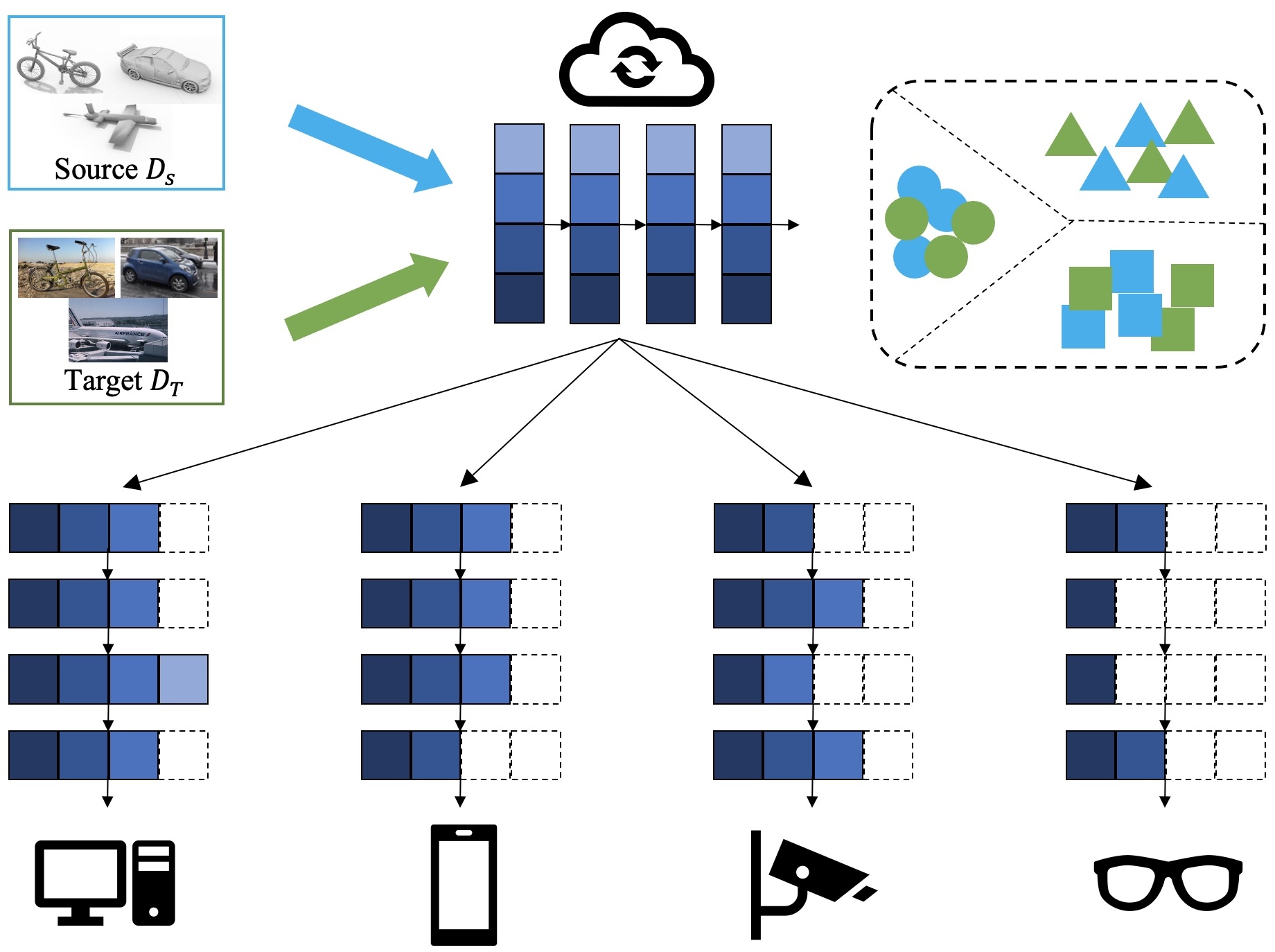
Refer to caption — Figure 1: SlimDA: We only adapt once on cloud computing center but can flexibly sample models with diverse capacities to distribute to different resource-limited edge devices.

Vanilla UDA aims to align source data and target data into a joint representation space so that the model trained on source data can be well generalized to target data [32, 13, 55, 47, 37, 24, 8]. Unfortunately, there is still a gap between academic studies and industrial needs: most existing UDA methods only perform weight adaptation with fixed neural architecture yet cannot fit the requirements of various devices in the real-world applications efficiently. Taking the example of a widely-used application scenario as shown in Fig.1, a domain adaptive model trained on a powerful cloud computing center is urged to be distributed to different resource-limited edge devices like laptops, smart mobile phones, and smartwatches, for real-time processing. In this scenario, vanilla UDA methods have to train a series of models with different capacities and architectures time-and-again to fit the requirements of devices with different computation budgets, which is expensive and time-consuming. To remedy the aforementioned issue, we propose Slimmable Domain Adaptation (SlimDA), in which we only train our model once so that the customized models with different capacities and architectures can be sampled flexibly from it to supply the demand of devices with different computation budgets.

Although slimmable neural networks [67, 66, 65] had been studied in the supervised tasks, in which models with different layer widths (i.e., channel number) can be coupled into a weight-sharing model bank for optimization, there remain two challenges when slimmable neural networks meet unsupervised domain adaptation: 1) Weight adaptation: How to simultaneously boost the adaptation performance of all models in the model bank? 2) Architecture adaptation: Given a specific computational budget, how to search an appropriate model on the unlabeled target data?

Methods	Data Type	Teacher	Student	Model
CKD	Labeled	Single	Single	Fixed
SEED	Unlabeled	Multiple	Multiple	Stochastic

Table 1: Conventional Knowledge Distillation (CKD) vs. Stochastic EnsEmble Distillation (SEED).

For the first challenge, there is a straightforward baseline in which UDA methods are directly applied to each model sampled from the model bank. However, this paradigm neglects to exploit the complementary knowledge among tremendous neural architectures in the model bank. To remedy this issue, we propose Stochastic EnsEmble Distillation (SEED) to interact the models in the model bank so as to suppress the uncertainty of intra-model adaptation on the unlabeled target data. SEED is a curriculum mutual learning framework in which the expectation of the predictions from stochastically-sampled models are exploited to assist domain adaptation of the model bank. The differences between SEED and the conventional knowledge distillation are shown in Table 1. As for intra-model adaptation, we borrow the solution from the state-of-the-art bi-classifier-based domain confusion method (such as SymNet [69] and MCD [47]). Nevertheless, we analyze that there exists an optimization conflict between inter-model interaction and intra-model adaptation, which motivates us to augment an Optimization-Separated Tri-Classifier (OSTC) to modulate the optimization between them.

For the second challenge, it is intuitive to search models with optimal adaptation performance under different computational budgets after training the model bank. However, unlike performance evaluation in the supervised tasks, none of the labeled target data is available. To be compatible with the unlabeled target data, we exploit the model with the largest capacity as an anchor to guide performance ranking in the model bank, since the larger models tend to be more accurate as empirically proven in [63]. In this way, we propose an Unsupervised Performance Evaluation Metric which is eased into the output discrepancy between the candidate model and the anchor model. The smaller the metric is, the better the performance is assumed to be.

Extensive ablation studies and experiments are carried out on three popular UDA benchmarks, i.e., ImageCLEF-DA [35], Office-31 [45], and Office-Home [56], which demonstrate the effectiveness of the proposed framework. Our method can achieve state-of-the-art results compared with other competing methods. It is worth emphasizing that our method can preserve the performance improvement against the source-only model even when the computing complexity is reduced to $1/64\times$ . To summarize, our main contributions are listed as follows:

•

We propose SlimDA, a “once-for-all” framework to jointly accommodate the adaptation performance and the computation budgets for resource-limited devices.
•

We propose SEED to simultaneously boost the adaptation performance of all models in the model bank. In particular, we design an Optimization-Separated Tri-Classifier to modulate the optimization between intra-model adaptation and inter-model interaction.
•

We propose an Unsupervised Performance Evaluation Metric to facilitate architecture adaptation.
•

Extensive experiments verify the effectiveness of our proposed SlimDA framework, which can surpass other state-of-the-art methods by a large margin.

2 Related Work

2.1 Unsupervised Domain Adaptation

Existing UDA methods aim to improve the model performance on the unlabeled target domain. In the past few years, discrepancy-based methods [32, 52, 18] and adversarial optimization methods [47, 31, 1, 22, 13] are proposed to solve this problem via domain alignment. Specifically, SymNet [69] develops a bi-classifier architecture to facilitate category-level domain confusion. Recently, Li et.al. [25] attempts to learn optimal architectures to further boost the performance on the target domain, which proves the significance of network architecture for UDA. These UDA methods focus on achieving a specific model with better performance on the target domain.

2.2 Neural Architecture Search

Neural Architecture Search (NAS) methods aim to search for optimal architectures automatically through reinforcement learning [70, 5, 71, 54, 53], evolution methods [30, 44, 43, 11], gradient-based methods [51, 38, 29, 58, 60] and so on. Recently, one-shot methods [65, 41, 16, 3, 60, 2] are very popular since only one super-network is required to train, and numerous weight-sharing sub-networks of various architectures are optimized simultaneously. In this way, the optimal network architecture can be searched from the model bank. In this paper, we highlight that UDA is an unnoticed yet significant scenario for NAS, since they can be cooperated to optimize a scene-specific lightweight architecture in an unsupervised way.

2.3 Cross-domain Network Compression

Chen et.al. [7] proposes a cross-domain unstructured pruning method. Yu et.al. [64] adopts MMD [32] to minimize domain discrepancy and prunes filters in a Taylor-based strategy, and Yang et.al. [62, 61] focuses on compressing graph neural networks. Feng et.al. [12] conducts adversarial training between the channel-pruned network and the full-size network. However, the performances of the existing methods still have a great improvement space. Moreover, their methods are not flexible enough to obtain numerous optimal models under diverse resource constraints.

3 Preliminary

3.1 Bi-Classifier Based Domain Confusion

3.1.1 Notation

A labeled source data $\mathcal{D}_{s}=\{(x_{i}^{s},y_{i}^{s})\}_{i=1}^{n_{s}}$ and an unlabeled target data $\mathcal{D}_{t}=\{(x_{i}^{t})\}_{i=1}^{n_{t}}$ are provided for training. SymNet [69] is composed of a feature extractor $F$ and two task classifiers $C^{s}$ and $C^{t}$ . A novel design in SymNet is to construct a new classifier $C^{st}$ which shares the neurons with $C^{s}$ and $C^{t}$ . $C^{st}$ is designed for domain discrimination and domain confusion without an explicit domain discriminator. The probability outputs of $C^{s}$ , $C^{t}$ and $C^{st}$ are $\mathbf{g}(x;F,C^{s})\in[0,1]^{K}$ , $\mathbf{g}(x;F,C^{t})\in[0,1]^{K}$ and $\mathbf{g}(x;F,C^{st})\in[0,1]^{2K}$ respectively, where $K$ is the class number of the task. The $k^{th}$ element of the probability output can be written as $\mathbf{g}_{k}^{s}(x)$ , $\mathbf{g}_{k}^{t}(x)$ and $\mathbf{g}_{k}^{st}(x)$ , respectively.

3.1.2 Task and Domain Discrimination

The training objective of task discrimination for $C^{s}$ & $C^{t}$ is:

\displaystyle\min_{C^{s},C^{t}}-\frac{1}{n_{s}}\sum_{i=1}^{n_{s}}\log(\mathbf{g}_{y_{i}^{s}}^{s}(x_{i}^{s}))-\frac{1}{n_{s}}\sum_{i=1}^{n_{s}}\log(\mathbf{g}_{y_{i}^{s}}^{t}(x_{i}^{s}))

(1)

The training objective of domain discrimination for $C^{st}$ is:

\min_{C^{st}}-\frac{1}{n_{s}}\sum_{i=1}^{n_{s}}\log{\sum_{k=1}^{K}\mathbf{g}_{k}^{st}(x_{i}^{s})}-\frac{1}{n_{t}}\sum_{i=1}^{n_{t}}\log{\sum_{k=1}^{K}\mathbf{g}_{k+K}^{st}(x_{i}^{t})}

(2)

3.1.3 Category-Level Domain Confusion

The training objective of category-level confusion is:

\min_{F}-\frac{1}{2n_{s}}\sum_{i=1}^{n_{s}}\log(\mathbf{g}_{y_{i}^{s}}^{st}(x_{i}^{s}))-\frac{1}{2n_{s}}\sum_{i=1}^{n_{s}}\log(\mathbf{g}_{y_{i}^{s}+K}^{st}(x_{i}^{s}))

(3)

The training objective of domain-level confusion is:

\min_{F}-\frac{1}{2n_{t}}\sum_{i=1}^{n_{t}}\log(\sum_{k=1}^{K}\mathbf{g}_{k}^{st}(x_{i}^{t}))-\frac{1}{2n_{t}}\sum_{i=1}^{n_{t}}\log(\sum_{k=1}^{K}\mathbf{g}_{k+K}^{st}(x_{i}^{t}))

(4)

Besides, an entropy minimization loss is conducted on $\mathcal{D}_{t}$ to optimize $F$ . For more detailed technical illustration, we recommend referring to the original paper.

4 Method

4.1 Straightforward Baseline

It has been proven in slimmable neural networks that numerous networks with different widths (i.e., layer channel) can be coupled into a weight-sharing model bank and be optimized simultaneously. We begin with a baseline in which SymNet is straightforwardly merged with the slimmable neural networks. The overall objective of SymNet is unified as $\mathcal{L}_{dc}$ for simplicity. In each training iteration, several models can be stochastically sampled from the model bank $\{(F_{j},C_{j}^{s},C_{j}^{t})\}_{j=1}^{m}$ $\in$ $(F,C^{s},C^{t})$ , named as model batch, where $m$ represents the model batch size. Here $(F,C^{s},C^{t})$ can be viewed as the largest model, and the remaining models can be sampled from it in a weight-sharing manner. To make sure the model bank can be fully trained, the largest and the smallest models^*^**The smallest model corresponds to 1/64 $\times$ FLOPs model (1/8 $\times$ channels) by default in this paper. should be sampled and constituted as a part of model batch in each training iteration. (Note that each model should re-calculate the statistical parameters of BN layers before deploying).

\displaystyle\bigg{(}\frac{\partial\mathcal{L}_{dc}}{\partial C^{s}},\frac{\partial\mathcal{L}_{dc}}{\partial C^{t}}\bigg{)}\!\!=\!\!\bigg{(}\frac{1}{m}\sum_{j=1}^{m}\frac{\partial\mathcal{L}_{dc}}{\partial C^{s}_{j}},\frac{1}{m}\sum_{j=1}^{m}\frac{\partial\mathcal{L}_{dc}}{\partial C^{t}_{j}}\bigg{)}

(5)

\displaystyle\frac{\partial\mathcal{L}_{dc}}{\partial F}=\frac{1}{m}\sum_{j=1}^{m}\frac{\partial\mathcal{L}_{dc}}{\partial F_{j}}

(6)

This baseline can be viewed as two alternated processes of Eqn.5 and Eqn.6 to optimize the model bank. To encourage inter-model interaction in the above baseline, we propose our SlimDA framework as shown in Fig. 2.

4.2 Stochastic EnsEmble Distillation

Stochastic Ensemble: It is intuitive that different models in the model bank can learn complementary knowledge about the unlabeled target data. Inspired by Bayesian learning with model perturbation, we exploit the models in the model bank via Monte Carlo Sampling to suppress the uncertainty from unlabeled target data. The expected prediction $\mathbf{g}_{seed}(x_{i}^{t})$ can be approximated by taking the expectation of $\{\mathbf{g}(x_{i};F_{j},C_{j}^{s},C_{j}^{t})\}_{j=1}^{m}$ with respect to the model confidence $\{\mathbf{g}(F_{j},C_{j}^{s},C_{j}^{t})\}_{j=1}^{m}$ ^†^†† $\mathbf{g}(F_{j},C_{j}^{s},C_{j}^{t})$ is short for $\mathbf{g}(F_{j},C_{j}^{s},C_{j}^{t}\,|\,\mathcal{D})$ where $\mathcal{D}$ denotes the training data. The model confidence, ranging [0,1], can be interpreted to measure the relative accuracy among the models in the model bank.:

\displaystyle\mathbf{g}_{seed}(x_{i}^{t})=\mathbb{E}_{\mathbf{g}(F_{j},C_{j}^{s},C_{j}^{t})}\big{[}\mathbf{g}(x_{i}^{t};F_{j},C_{j}^{s},C_{j}^{t})\big{]}

(7)

\displaystyle\mathbf{g}(x_{i}^{t};F_{j},C_{j}^{s},C_{j}^{t})=\frac{1}{2}(\mathbf{g}(x_{i}^{t};F_{j},C_{j}^{s})+\mathbf{g}(x_{i}^{t};F_{j},C_{j}^{t}))

(8)

where $\mathbb{E}$ is a weighted average function with $j$ $=$ $\{1,...,m\}$ , and the subscript of $\mathbb{E}$ denotes the weight.

Assumption 4.1

As demonstrated by extensive empirical results in in-domain generalization work [63] and out-of-domain generalization work [6], the models with larger capacity^‡^‡‡We use FLOPs as a metric to measure model capacity in this paper. perform more accurate than those with smaller capacity statistically. Thus, it is reasonable to assume that $\mathbf{g}(F_{1},C_{1}^{s},C_{1}^{t})\geq\mathbf{g}(F_{2},C_{2}^{s},C_{2}^{t})\geq...\geq\mathbf{g}(F_{m},C_{m}^{s},C_{m}^{t})$ where the index denotes the order of model capacity from large to small.

In this work, we empirically define the model confidence in a hard way:

		$\displaystyle r_{j}=\frac{\mathcal{M}(F_{j},C_{j}^{s},C_{j}^{t})}{\mathcal{M}(F,C^{s},C^{t})}$		(9)
		$\displaystyle\Omega=\{(F_{j},C_{j}^{s},C_{j}^{t})\ \ {\rm whose}\ \ r_{j}\geq\lambda\}$
		$\displaystyle\mathbf{g}(F_{j},C_{j}^{s},C_{j}^{t})=\left\{\begin{aligned} &1\ ,\ {\rm if}\ \ (F_{j},C_{j}^{s},C_{j}^{t})\in\Omega\\ &0\ ,\ {\rm otherwise}\end{aligned}\right.$

where $\lambda$ is set 0.5 by default, and $\mathcal{M}(\cdot)$ represents the model capacity. As the prediction tends to be uncertain on the unlabeled target data, we aim to produce lower-entropy predictions to boost the discrimination [15]. In this work, we apply a sharpening function to $\mathbf{g}_{seed}(x_{i}^{t})$ to induce implicit entropy minimization during SEED training:

\mathbf{g}_{seed,k}(x_{i}^{t})=\mathbf{g}_{seed,k}(x_{i}^{t})^{\frac{1}{\tau}}/\sum_{k^{\prime}=1}^{K}\mathbf{g}_{seed,k^{\prime}}(x_{i}^{t})^{\frac{1}{\tau}}

(10)

where $\tau$ is a temperature parameter for sharpening, and is set $0.5$ by default in this paper. $\mathbf{g}_{seed}(x_{i}^{t})$ is used to refine the model batch, along with domain confusion training in a curriculum mutual learning manner.

Distillation Bridged by Optimization-Separated Tri-Classifier: We cannot directly feed $\mathbf{g}_{seed}(x_{i}^{t})$ back to the original bi-classifier for distillation since there exists optimization conflict between intra-model adaptation (Eqn.1-4) and inter-model interaction (distillation by $\mathbf{g}_{seed}(x_{i}^{t})$ ) in the model bank, which are two asynchronous tasks. Specifically, in the $q$ iteration, domain confusion bi-classifier of multi-models provides two-part information, including task discrimination and domain-confusion, and the two information are aggregated in $\mathbf{g}_{seed}^{q}(x_{i}^{t})$ . In the next $q$ +1 iteration, the above information can be further updated via the bi-classifier training. However, if we transfer $\mathbf{g}_{seed}^{q}(x_{i}^{t})$ back to the bi-classifier, $\mathbf{g}_{seed}^{q}(x_{i}^{t})$ will offset the gains of the two information in $\mathbf{g}_{seed}^{q+1}(x_{i}^{t})$ and hinder the refinement of $\mathbf{g}_{seed}(x_{i}^{t})$ . Thus, the curriculum learning in our SlimDA framework will be destroyed.

To this end, we introduce an Optimization-Separated Tri-Classifier (OSTC) $\{(C_{j}^{s},C_{j}^{t},C_{j}^{a})\}_{j=1}^{m}$ $\in$ $(C^{s},C^{t},C^{a})$ , where the former two are preserved for domain confusion training, and the last one is designed to receive the stochastically-aggregated knowledge for distillation. The distillation loss is formulated as:

	$\displaystyle\mathcal{L}_{seed}=$	$\displaystyle-\frac{1}{m\times n_{t}}\sum_{j=1}^{m}\sum_{i=1}^{n_{t}}\mathbf{g}_{seed}(x_{i}^{t})\log(\mathbf{g}(x_{i}^{t};F_{j},C_{j}^{a}))$		(11)
		$\displaystyle-\frac{1}{m\times n_{s}}\sum_{j=1}^{m}\sum_{i=1}^{n_{s}}\textbf{1}_{y_{i}^{s}}\log(\mathbf{g}(x_{i}^{s};F_{j},C_{j}^{a}))$		(11)

We optimize $(C^{s},C^{t},C^{a})$ with $\mathcal{L}_{dc}$ and $\mathcal{L}_{seed}$ losses:

	$\displaystyle\bigg{(}\frac{\partial\mathcal{L}_{dc}}{\partial C^{s}},\frac{\partial\mathcal{L}_{dc}}{\partial C^{t}}\bigg{)}$	$\displaystyle=\bigg{(}\frac{1}{m}\sum_{j=1}^{m}\frac{\partial\mathcal{L}_{dc}}{\partial C^{s}_{j}},\frac{1}{m}\sum_{j=1}^{m}\frac{\partial\mathcal{L}_{dc}}{\partial C^{t}_{j}}\bigg{)}$		(12)
	$\displaystyle\frac{\partial\mathcal{L}_{seed}}{\partial C^{a}}$	$\displaystyle=\frac{1}{m}\sum_{j=1}^{m}\frac{\partial\mathcal{L}_{seed}}{\partial C_{j}^{a}}$		(12)

As to optimize $F$ , we use the model confidence in Eqn.9 to modulate the training objectives of $\mathcal{L}_{dc}$ and $\mathcal{L}_{seed}$ :

\displaystyle\begin{split}\frac{\partial\mathcal{L}_{total}}{\partial F}=&\mathbb{E}_{\mathbf{g}(F_{j},C_{j}^{s},C_{j}^{t})}\big{[}\frac{\partial\mathcal{L}_{dc}}{\partial F_{j}}\big{]}\\ &+\mathbb{E}_{1-\mathbf{g}(F_{j},C_{j}^{s},C_{j}^{t})}\big{[}\frac{\partial\mathcal{L}_{seed}}{\partial F_{j}}\big{]}\end{split}

(13)

To summarize, the OSTC in Eqn.12 and the feature extractor in Eqn.13 are optimized in an alternated way in each training iteration. Once finishing training, $(C^{s},C^{t})$ are discarded and only $C^{a}$ is retained to deploy more efficiently.

Model batch size	I $\to$ P	P $\to$ I	I $\to$ C	C $\to$ I	C $\to$ P	P $\to$ C	Avg.
2 (w/ CKD)	71.8	83.3	93.0	82.2	67.3	89.2	81.1
2	73.5	88.3	92.2	87.1	69.3	91.5	83.7
4	74.3	89.0	92.6	87.5	69.8	92.0	84.2
6	75.3	90.2	94.1	88.3	71.7	94.2	85.6
8	76.1	89.9	94.9	88.1	71.7	94.2	85.8
10	78.3	90.7	95.8	88.3	71.8	94.8	86.6

Table 2: Two ablation studies on ImageCLEF-DA: 1) The second row represents the results from conventional knowledge distillation (CKD). 2) Comparison among different model batch sizes in SlimDA. We report the above results for

1/64\times

models.

Baseline	SEED	OSTC	1 $\times$	1/2 $\times$	1/4 $\times$	1/8 $\times$	1/16 $\times$	1/32 $\times$	1/64 $\times$
✓			88.6	88.0	86.9	86.0	84.1	82.0	81.7
✓	✓		87.9	87.6	87.3	86.9	86.5	86.1	85.9
✓	✓	✓	88.9	88.7	88.8	88.4	88.3	87.2	86.6

Table 3: The ablation studies for the components in SlimDA on ImageCLEF-DA dataset.

Methods	1 $\times$	1/2 $\times$	1/4 $\times$	1/8 $\times$	1/16 $\times$	1/32 $\times$	1/64 $\times$
SymNet w/o SlimDA	78.9	77.0	76.7	74.8	71.2	68.2	69.3
SymNet w/ SlimDA	79.2	79.0	79.0	78.7	78.8	78.2	78.3
improvement	0.3 $\uparrow$	2.0 $\uparrow$	2.3 $\uparrow$	3.9 $\uparrow$	7.6 $\uparrow$	10.0 $\uparrow$	9.0 $\uparrow$
MCD w/o SlimDA	77.2	75.0	75.0	72.3	70.3	68.7	69.6
MCD w/ SlimDA	78.5	78.2	78.1	78.0	77.7	77.6	77.7
improvement	1.3 $\uparrow$	3.2 $\uparrow$	3.1 $\uparrow$	5.7 $\uparrow$	7.4 $\uparrow$	8.9 $\uparrow$	8.1 $\uparrow$
STAR w/o SlimDA	76.9	74.0	69.7	68.1	65.6	62.9	64.7
STAR w/ SlimDA	77.8	77.5	77.2	77.2	77.0	76.9	77.0
improvement	0.9 $\uparrow$	3.5 $\uparrow$	7.5 $\uparrow$	9.1 $\uparrow$	11.4 $\uparrow$	14.0 $\uparrow$	12.3 $\uparrow$

Table 4: Two ablation studies on ImageCLEF-DA for I

\to

P adaptation task: 1) Comparison with different UDA methods injected into SlimDA, which indicates the universality of our framework. 2) Comparison with stand-alone networks (aka “w/o SlimDA”), which have the same architectures as our searched models but are trained individually outsides the model bank.

Methods	#Params	FLOPs	I $\to$ P	P $\to$ I	I $\to$ C	C $\to$ I	C $\to$ P	P $\to$ C	Avg.
ShuffleNetV2 [40]	2.3M	146M	63.2	65.4	82.1	81.0	65.2	78.9	72.6
MobileNetV3 [23]	5.4M	219M	72.8	85.3	93.2	80.3	65.0	91.7	81.4
GhostNet [19]	5.2M	141M	75.8	89.5	95.5	86.1	70.2	94.0	85.2
MobileNetV2 [49]	3.5M	300M	76.0	90.6	95.1	87.0	69.1	95.1	85.5
EfficientNet_B0 [54]	5.3M	390M	76.5	88.5	96.5	87.3	71.3	94.0	85.6
SlimDA ( $1/8\times$ ResNet-50)	4.0M	517M	78.7	91.7	97.2	90.5	75.8	96.2	88.4
SlimDA ( $1/64\times$ ResNet-50)	1.6M	64M	78.3	90.7	95.8	88.3	71.8	94.8	86.6

Table 5: Performance comparison with different state-of-the-art lightweight networks on ImageCLEF-DA dataset.

4.3 Unsupervised Performance Evaluation Metric

In the context of UDA, one of the challenging points is to evaluate the performance ranking of models on the unlabeled target data rather than the searching methods. According to the Triangle Inequality Theorem, we can obtain the relationship among the predictions of the candidate model $(F_{j},C_{j}^{a})$ , the largest model $(F,C^{a})$ , as well as the ground-truth label:

\displaystyle\begin{split}&\parallel\mathbf{g}(\mathcal{D}_{t};F_{j},C_{j}^{a})\!\!-\!\!GT(\mathcal{D}_{t})\parallel_{2}^{2}<\parallel\mathbf{g}(\mathcal{D}_{t};F,C^{a})\!\!-\!\!GT(\mathcal{D}_{t})\parallel_{2}^{2}\\ &\!\!+\!\!\parallel\mathbf{g}(\mathcal{D}_{t};F_{j},C_{j}^{a})\!\!-\mathbf{g}(\mathcal{D}_{t};F,C^{a})\parallel_{2}^{2}\end{split}

(14)

where $GT(\mathcal{D}_{t})$ denotes the ground-truth label of the target data. According to the assumption ‡ ‣ 4.1, the model with the largest capacity tends to be the most accurate in the model bank, which means:

\parallel\mathbf{g}(\mathcal{D}_{t};F_{j},C_{j}^{a})\!\!-\!\!GT(\mathcal{D}_{t})\parallel_{2}^{2}>\parallel\mathbf{g}(\mathcal{D}_{t};F,C^{a})\!\!-\!\!GT(\mathcal{D}_{t})\parallel_{2}^{2}

(15)

Combining Eqn.14 and Eqn.15, we can take the model with the largest capacity as an anchor to compare the performance of candidate models on the unlabeled target data. The Unsupervised Performance Evaluation Metric (UPEM) for each model can be written as:

\Delta_{j}=\parallel\mathbf{g}(\mathcal{D}^{t};F_{j},C_{j}^{a})-\mathbf{g}(\mathcal{D}^{t};F,C^{a})\parallel_{2}^{2}\vspace{-1mm}

(16)

where $\Delta_{j}$ is the $\mathcal{L}$ 2 distance between outputs of the candidate model and the anchor model. With the UPEM, we can use a greedy search method [65, 41] for neural architecture search (Note that we can also use other search methods, but this is not the deciding point in this paper).

Methods	#Params	FLOPs	I $\to$ P	P $\to$ I	I $\to$ C	C $\to$ I	C $\to$ P	P $\to$ C	Avg.	$\Delta$
Source Only [69]	1 $\times$	1 $\times$	74.8	83.9	91.5	78.0	65.5	91.2	80.7	–
DAN [32]	1 $\times$	1 $\times$	74.5	82.2	92.8	86.3	69.2	89.8	82.5	–
RevGrad [13]	1 $\times$	1 $\times$	75.0	86.0	96.2	87.0	74.3	91.5	85.0	–
MCD [47] (impl.)	1 $\times$	1 $\times$	77.2	87.2	93.8	87.7	71.8	92.5	85.0	–
STAR [37] (impl.)	1 $\times$	1 $\times$	76.9	87.7	93.8	87.6	72.1	92.7	85.1	–
CDAN+E [36]	1 $\times$	1 $\times$	77.7	90.7	97.7	91.3	74.2	94.3	87.7	–
SymNets [69]	1 $\times$	1 $\times$	80.2	93.6	97.0	93.4	78.7	96.4	89.9	–
SymNets (impl.)	1 $\times$	1 $\times$	78.8	92.2	96.7	91.0	76.0	96.2	88.5	–
TCP [64]	1/1.7 $\times$	–	75.0	82.6	92.5	80.8	66.2	86.5	80.6	–
	1/2.5 $\times$	–	67.8	77.5	88.6	71.6	57.7	79.5	73.8	–
ADMP [12]	1/1.7 $\times$	–	77.3	90.2	90.2	95.8	88.9	73.7	86.3	–
	1/2.5 $\times$	–	77.0	89.5	95.5	88.9	72.3	91.2	85.7	–
SlimDA	1 $\times$	1 $\times$	79.2	92.3	97.5	91.2	76.7	96.5	88.9	–
	1/1.9 $\times$	1/2 $\times$	79.0	92.3	97.3	90.8	76.8	96.2	88.7	0.2 $\downarrow$
	1/3.9 $\times$	1/4 $\times$	79.0	92.2	97.3	90.8	77.2	96.3	88.8	0.1 $\downarrow$
	1/9.4 $\times$	1/8 $\times$	78.7	91.7	97.2	90.5	75.8	96.2	88.4	0.5 $\downarrow$
	1/12.8 $\times$	1/16 $\times$	78.8	91.5	97.3	90.2	76.0	96.2	88.3	0.6 $\downarrow$
	1/28.8 $\times$	1/32 $\times$	78.2	90.5	96.7	89.3	72.2	96.0	87.2	1.7 $\downarrow$
	1/64 $\times$	1/64 $\times$	78.3	90.7	95.8	88.3	71.8	94.8	86.6	2.3 $\downarrow$

Table 6: Performance on the ImageCLEF-DA dataset. “–” means that the results are not reported in the original paper. “impl.” denotes our re-implementation using the released code. “

\Delta

” indicates the performance gap between the searched model and ResNet-50 based model for each UDA method. TCP and ADMP are two related cross-domain network compression methods. We adapt the architectures for six adaptation tasks under seven computational constraints (FLOPs). Since the model architectures adapted for different tasks are different even with the same FLOPs, we calculate the parameter reduction (#Params) by averaging models in 6 adaptation tasks.

Methods	#Params	FLOPs	A $\to$ W	D $\to$ W	W $\to$ D	A $\to$ D	D $\to$ A	W $\to$ A	Avg.	$\Delta$
Source Only [69]	$1\times$	$1\times$	79.9	96.8	99.5	84.1	64.5	66.4	81.9	–
Domain Confusion [21]	$1\times$	$1\times$	83.0	98.5	99.8	83.9	66.9	66.4	83.1	–
Domain Confusion+Em [21]	$1\times$	$1\times$	89.8	99.0	100.0	90.1	73.9	69.0	87.0	–
BNM [9]	$1\times$	$1\times$	91.5	98.9	100.0	90.3	70.9	71.6	87.1	–
DMP [39]	$1\times$	$1\times$	93.0	99.0	100.0	91.0	71.4	70.2	87.4	–
DMRL [59]	$1\times$	$1\times$	90.8	99.0	100.0	93.4	73.0	71.2	87.9	–
SymNets [69]	$1\times$	$1\times$	90.8	98.8	100.0	93.9	74.6	72.5	88.4	–
SymNets (impl.)	$1\times$	$1\times$	91.0	98.4	99.6	89.7	72.2	72.5	87.2	–
TCP [64]	1/1.7 $\times$	–	81.8	98.2	99.8	77.9	50.0	55.5	77.2	–
	1/2.5 $\times$	–	77.4	96.3	100.0	72.0	36.1	46.3	71.3	–
ADMP [12]	1/1.7 $\times$	–	83.3	98.9	99.9	83.1	63.2	64.2	82.0	–
	1/2.5 $\times$	–	82.1	98.6	99.9	81.5	63.0	63.2	81.3	–
SlimDA	1 $\times$	1 $\times$	90.7	91.2	91.1	99.8	73.7	71.0	87.6	–
	1/2 $\times$	1/2 $\times$	90.7	99.1	100.0	91.8	73.3	71.1	87.6	0.0 $\downarrow$
	1/4 $\times$	1/4 $\times$	90.5	98.1	99.8	91.9	73.1	71.2	87.4	0.2 $\downarrow$
	1/10 $\times$	1/8 $\times$	90.6	98.8	100.0	91.6	72.9	71.1	87.5	0.1 $\downarrow$
	1/14 $\times$	1/16 $\times$	90.5	98.7	99.8	91.4	73.1	71.0	87.4	0.2 $\downarrow$
	1/20 $\times$	1/32 $\times$	90.8	97.7	99.5	91.5	71.8	70.8	87.0	0.6 $\downarrow$
	1/64 $\times$	1/64 $\times$	91.2	97.2	98.9	91.2	71.3	68.9	86.8	0.8 $\downarrow$

Table 7: Performance on the Office-31 dataset. As for other illustrations, please refer to the caption of Table 6.

5 Experiments

5.1 Dataset

ImageCLEF-DA [32] consists of 1,800 images with 12 categories over three domains: Caltech-256 (C), ImageNet ILSVRC 2012 (I), and Pascal VOC 2012 (P).

Office-31 [46] is a popular benchmark with about 4,110 images sharing 31 categories of daily objects from 3 domains: Amazon (A), Webcam (W) and DSLR (D).

Office-Home [57] contains 15,500 images sharing 65 categories of daily objects from 4 different domains: Art (Ar), Clipart (Cl), Product (Pr), and Real-World (Rw).

5.2 Model Bank Configurations

Following the exiting methods [7, 12, 64], we select ResNet-50 [20] as the main network to conduct the following experiments. Unlike these methods, the ResNet-50 adopted in this paper is a super-network that couples numerous models with different layer widths to form the model bank. Identical to these methods, the super-network should be firstly pre-trained on ImageNet and then fine-tuned on the downstream tasks.

5.3 Implementation Details

An SGD optimizer with momentum of 0.9 is adopted to train all UDA tasks in this paper. Following [69], the learning rate is adjusted by $l=l_{0}/(1+\alpha p)^{\beta}$ , where $l_{0}=0.01$ , $\alpha=10$ , $\beta=0.75$ , and $p$ varies from $0$ to $1$ linearly with the training epochs. The training epoch is set 40. The training and testing image resolution is $224\times 224$ . An important technical detail is that, before performance evaluation, the models sampled in the model bank should update the statistic of their BN layers on the target domain via AdaBN [26]. We mainly take the computational complexity (FLOPs) as resource constraint for architecture adaptation, and set 1/64 $\times$ FLOPs as the smallest model by default.

Methods	FLOPs	Ar $\to$ Cl	Ar $\to$ Pr	Ar $\to$ Rw	Cl $\to$ Ar	Cl $\to$ Pr	Cl $\to$ Rw	Pr $\to$ Ar	Pr $\to$ Cl	Pr $\to$ Rw	Rw $\to$ Ar	Rw $\to$ Cl	Rw $\to$ Pr	Avg.	$\Delta$
Source Only	$1\times$	34.9	50.0	58.0	37.4	41.9	46.2	38.5	31.2	60.4	53.9	41.2	59.9	46.1	–
DAN	$1\times$	43.6	57.0	67.9	45.8	56.5	60.4	44.0	43.6	67.7	63.1	51.5	74.3	56.3	–
RevGrad	$1\times$	45.6	59.3	70.1	47.0	58.5	60.9	46.1	43.7	68.5	63.2	51.8	76.8	57.6	–
CDAN-E	$1\times$	50.7	70.6	76.0	57.6	70.0	70.0	57.4	50.9	77.3	70.9	56.7	81.6	65.8	–
SymNet	$1\times$	47.7	72.9	78.5	64.2	71.3	74.2	64.2	48.8	79.5	74.5	52.6	82.7	67.6	–
BNM	$1\times$	52.3	73.9	80.0	63.3	72.9	74.9	61.7	49.5	79.7	70.5	53.6	82.2	67.9	–
SlimDA	1 $\times$	52.8	72.3	77.2	63.5	72.3	73.3	64.8	52.2	79.7	72.4	57.8	82.8	68.4	–
	1/2 $\times$	52.4	72.0	77.2	62.8	72.0	73.0	65.1	53.2	79.4	72.1	55.3	82.0	68.0	0.4 $\downarrow$
	1/4 $\times$	51.9	71.8	77.1	62.4	71.9	72.3	64.8	53.1	78.8	71.9	55.1	82.1	67.8	0.6 $\downarrow$
	1/8 $\times$	51.6	71.4	76.6	62.5	71.0	71.0	65.0	53.0	78.4	71.5	55.2	81.6	67.4	1.0 $\downarrow$
	1/16 $\times$	51.0	71.0	75.9	61.3	70.6	70.0	64.4	52.3	77.7	70.2	54.6	81.2	66.7	1.7 $\downarrow$
	1/32 $\times$	50.0	70.6	74.0	57.7	70.3	68.9	60.1	51.6	76.3	67.5	51.7	80.9	65.0	3.4 $\downarrow$
	1/64 $\times$	49.7	70.1	72.9	56.6	70.0	66.3	56.5	48.3	75.9	65.9	55.5	80.9	64.0	4.4 $\downarrow$

Table 8: Performance on the Office-Home dataset. As for other illustrations, please refer to the caption of Table 6.

5.4 Ablation Studies

5.4.1 Analysis for SEED

Comparison with Conventional Knowledge Distillation: As shown in Table 2, we can observe that our SEED with different model batch size can outperform the conventional knowledge distillation by a large margin even under 1/64 $\times$ FLOPs of ResNet-50 on ImageCLEF-DA.

Comparison among different model batch sizes: Model batch size is a vital hyper-parameter of our framework. Intuitively, a larger model batch is more sufficient to approximate the knowledge aggregation in the model bank. As shown in Table 2, a large model batch size is beneficial for our optimization method. We set the model batch size as 10 by default in our following experiments.

Comparison with stand-alone training: As shown in Table 4, compared with stand-alone training with the same network configuration, SEED can improve the overall adaptation performance by a large margin. Here “stand-alone” means that the models from $1\times$ to $1/64\times$ with the same topological configuration to the SlimDA counterparts are adapted individually outside the model bank. Specifically, not only the tiny models (from $1/2\times$ to $1/64\times$ ), but also the $1\times$ model trained with SEED outperform the corresponding stand-alone ones, which can be supported by more results in Table 6 and Table 7 (comparing the performance of $1\times$ models and our re-implemented ones).

Effectiveness of each component in our SlimDA: We conduct ablation studies to investigate the effectiveness of the components in our SlimDA framework. As shown in Table 3, the second row “Baseline” denotes the approach merging SymNet and slimmable neural network straightforwardly. We can observe that the SEED has a significant impact on the performance with fewer FLOPs, such as 1/4 $\times$ , 1/8 $\times$ , 1/16 $\times$ , 1/32 $\times$ , and 1/64 $\times$ , but the performances of 1 $\times$ and 1/2 $\times$ models with SEED fall 0.7% and 0.4%, respectively, compared with the baseline, which is attributed to the optimization conflict between intra-model domain confusion and inter-model SEED. The last row shows that our proposed OSTC provides an impressive improvement on the performance of large models (1 $\times$ and 1/2 $\times$ ) compared with both the SEED and baseline. Moreover, our proposed OSTC can further improve the performance of other models with fewer FLOPs. Overall, each component in SlimDA contributes to the performance-boosting of tiny models (from 1/64 $\times$ to 1/4 $\times$ ), the SEED w/o OSTC indeed brings negative transferring for models with larger capacity. However, our proposed OSTC can remedy the negative transferring issue and provide additional boosting under six FLOPs settings. The results in the ablation study also demonstrate the process of solving the challenges in our framework to accomplish the combination between UDA training and weight-sharing model bank.

5.4.2 Analysis for Architecture Adaptation

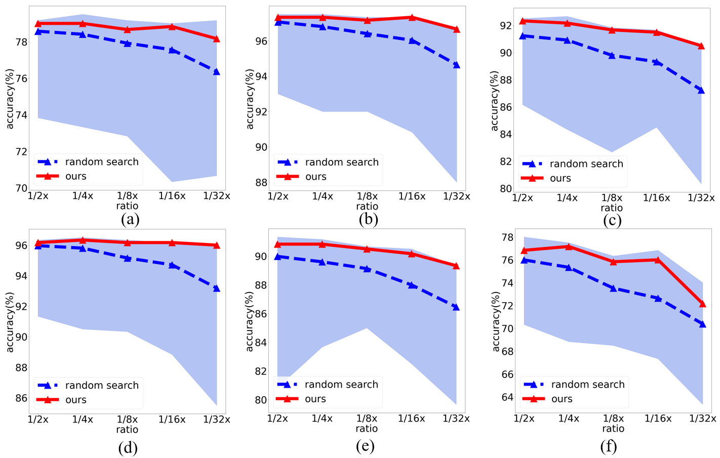
Analysis for UPEM: To validate the effectiveness of our proposed UPEM, we conduct 30 experiments which are composed of six adaptation tasks and five computational constraints. In each experiment, we sample 100 models in the model bank to evaluate the correlation between UPEM and the supervised accuracy with the ground-truth labels on target data. As shown in Fig.4, the Pearson correlation coefficients almost get close to $-1$ , which means the smaller the UPEM is, the higher the accuracy is.

Comparison with Random Search: As shown in Fig.3, the necessity of architecture adaptation is highlighted from the significant performance gap among random searched models under each computational budget. Meanwhile, the architectures searched for different tasks are different. Moreover, given the same computational budgets, models greedily searched from the model bank with our UPEM are the top series in their actual performance sorting.

5.4.3 Compatibility with Different UDA Methods

Our SlimDA can also be cooperated with other UDA approaches, such as MCD [47] and STAR [37]. To present the universality of our framework, we carry out additional experiments of SlimDA with MCD and STAR, as well as their stand-alone counterparts. As shown in Table 4, the results from our SlimDA with MCD and STAR are still superior to the corresponding stand-alone counterparts by a large margin, which further validates the effectiveness of our SlimDA framework from another perspective.

5.4.4 Convergence Performance

We sample different models for performance evaluation during model bank training. As shown in Fig.5, the models coupled in the model bank are optimized simultaneously. The performances are steadily improved as learning goes.

5.5 Comparisons with State-of-The-Arts

Comparison with UDA methods: We conduct extensive experiments on three popular domain adaptation datasets, including ImageCLEF-DA, Office-31, and Office-Home. Detailed results and performance comparison with SOTA UDA methods are presented in Table 6, Table 7 and Table 8. The benefits of our proposed SlimDA can be further pronounced when we reduce FLOPs extremely. Our method can preserve the accuracy improvement against the source-only model even when reducing FLOPs up to 1/64 $\times$ . As we can see in Table 6, Table 7 and Table 8, when we reduce FLOPs even up to 1/64 $\times$ , the accuracy on ImageCLEF-DA, Office-31 and Office-Home datasets only drop about 2.3%, 0.8% and 4.4%, respectively.

Comparision with cross-domain network compression methods: TCP [64] and ADMP [12] are two main cross-domain network compression methods for channel numbers, our method can significantly outperform them by a very large margin and achieve new SOTA results.

Comparison with lightweight networks: As shown in Table 5, not only human-designed lightweight networks like MobileNet series [49, 23], ShuffleNet [40] and GhostNet [19], but also auto-designed architectures like EfficientNet [54] is over-passed by our SlimDA with fewer FLOPs/parameters.

6 Conclusions

In this paper, we propose a simple yet effective SlimDA framework to facilitate weight and architecture joint-adaptation. In SlimDA, the proposed SEED exploits architecture diversity in a weight-sharing model bank to suppress prediction uncertainty on the unlabeled target data, and the proposed OSTC modulates the optimization conflict between intra-model adaptation and inter-model interaction. In this way, we can flexibly distribute resource-satisfactory models via a retrain-free sampling manner to various devices on target domain. Moreover, we propose UPEM to select the optimal cross-domain model under each computational budget. Extensive ablation studies and experiments are carried out to validate the effectiveness of SlimDA. Our SlimDA can also be extended to other visual computing tasks, such as object detection and semantic segmentation, which we leave as our future work. In short, our work provides a practical UDA framework towards real-world scenario, and we hope it can bring new inspirations to the widespread application of UDA.

Limitations. The assumption ‡ ‣ 4.1 is an essential prerequisite in this work, which will hold at least to a reasonable extent. However, it is not guaranteed theoretically, which may invalidate our method in some unknown circumstances.

Acknowledgements

This work was sponsored in part by National Natural Science Foundation of China (62106220, U20B2066), Hikvision Open Fund, AI Singapore (Award No.: AISG2-100E-2021-077), and MOE AcRF TIER-1 FRC RESEARCH GRANT (WBS: A-0009456-00-00).

References

[1] Konstantinos Bousmalis, Nathan Silberman, David Dohan, Dumitru Erhan, and Dilip Krishnan. Unsupervised pixel-level domain adaptation with generative adversarial networks. In CVPR, pages 3722–3731, 2017.
[2] Andrew Brock, Theodore Lim, James M Ritchie, and Nick Weston. Smash: one-shot model architecture search through hypernetworks. arXiv preprint arXiv:1708.05344, 2017.
[3] Han Cai, Chuang Gan, and S. Han. Once for all: Train one network and specialize it for efficient deployment. In ICLR, 2020.
[4] Han Cai, Chuang Gan, Tianzhe Wang, Zhekai Zhang, and Song Han. Once-for-all: Train one network and specialize it for efficient deployment. arXiv preprint arXiv:1908.09791, 2019.
[5] Han Cai, Jiacheng Yang, Weinan Zhang, Song Han, and Yong Yu. Path-level network transformation for efficient architecture search. arXiv preprint arXiv:1806.02639, 2018.
[6] P. Chattopadhyay, Y. Balaji, and J. Hoffman. Learning to balance specificity and invariance for in and out of domain generalization. 2020.
[7] Shangyu Chen, Wenya Wang, and Sinno Jialin Pan. Cooperative pruning in cross-domain deep neural network compression. In IJCAI, pages 2102–2108, 7 2019.
[8] Weijie Chen, Luojun Lin, Shicai Yang, Di Xie, Shiliang Pu, Yueting Zhuang, and Wenqi Ren. Self-supervised noisy label learning for source-free unsupervised domain adaptation. ArXiv, abs/2102.11614, 2021.
[9] Shuhao Cui, Shuhui Wang, Junbao Zhuo, Liang Li, Qingming Huang, and Qi Tian. Towards discriminability and diversity: Batch nuclear-norm maximization under label insufficient situations. In Proceedings of the IEEE/CVF Conference on Computer Vision and Pattern Recognition, pages 3941–3950, 2020.
[10] Shuhao Cui, Shuhui Wang, Junbao Zhuo, Chi Su, Qingming Huang, and Qi Tian. Gradually vanishing bridge for adversarial domain adaptation. In Proceedings of the IEEE/CVF Conference on Computer Vision and Pattern Recognition, pages 12455–12464, 2020.
[11] Thomas Elsken, Jan Hendrik Metzen, and Frank Hutter. Efficient multi-objective neural architecture search via lamarckian evolution. arXiv preprint arXiv:1804.09081, 2018.
[12] Xiaoyu Feng, Z. Yuan, G. Wang, and Yongpan Liu. Admp: An adversarial double masks based pruning framework for unsupervised cross-domain compression. ArXiv, abs/2006.04127, 2020.
[13] Yaroslav Ganin and Victor Lempitsky. Unsupervised domain adaptation by backpropagation. In ICML, pages 1180–1189, 2015.
[14] Yaroslav Ganin and Victor Lempitsky. Unsupervised domain adaptation by backpropagation. In International conference on machine learning, pages 1180–1189. PMLR, 2015.
[15] Yves Grandvalet, Yoshua Bengio, et al. Semi-supervised learning by entropy minimization. CAP, 367:281–296, 2005.
[16] Zichao Guo, X. Zhang, H. Mu, Wen Heng, Z. Liu, Y. Wei, and Jian Sun. Single path one-shot neural architecture search with uniform sampling. In ECCV, 2020.
[17] Zichao Guo, Xiangyu Zhang, Haoyuan Mu, Wen Heng, Zechun Liu, Yichen Wei, and Jian Sun. Single path one-shot neural architecture search with uniform sampling. In European Conference on Computer Vision, pages 544–560. Springer, 2020.
[18] Philip Haeusser, Thomas Frerix, Alexander Mordvintsev, and Daniel Cremers. Associative domain adaptation. In ICCV, pages 2765–2773, 2017.
[19] Kai Han, Yunhe Wang, Qi Tian, Jianyuan Guo, Chunjing Xu, and Chang Xu. Ghostnet: More features from cheap operations. In Proceedings of the IEEE/CVF Conference on Computer Vision and Pattern Recognition, pages 1580–1589, 2020.
[20] Kaiming He, Xiangyu Zhang, Shaoqing Ren, and Jian Sun. Deep residual learning for image recognition. In CVPR, 2016.
[21] Judy Hoffman, E. Tzeng, Trevor Darrell, and Kate Saenko. Simultaneous deep transfer across domains and tasks. 2015 IEEE International Conference on Computer Vision (ICCV), pages 4068–4076, 2015.
[22] Judy Hoffman, Eric Tzeng, Taesung Park, Jun-Yan Zhu, Phillip Isola, Kate Saenko, Alexei Efros, and Trevor Darrell. Cycada: Cycle-consistent adversarial domain adaptation. In ICML, pages 1989–1998, 2018.
[23] Andrew Howard, Mark Sandler, Grace Chu, Liang-Chieh Chen, Bo Chen, Mingxing Tan, Weijun Wang, Yukun Zhu, Ruoming Pang, Vijay Vasudevan, et al. Searching for mobilenetv3. In Proceedings of the IEEE/CVF International Conference on Computer Vision, pages 1314–1324, 2019.
[24] Xianfeng Li, Weijie Chen, Di Xie, Shicai Yang, and Yueting Zhuang. A free lunch for unsupervised domain adaptive object detection without source data. In AAAI, 2020.
[25] Yichen Li and Xingchao Peng. Network architecture search for domain adaptation. 2020.
[26] Yanghao Li, Naiyan Wang, Jianping Shi, Xiaodi Hou, and Jiaying Liu. Adaptive batch normalization for practical domain adaptation. Pattern Recognition, 80:109–117, 2018.
[27] Jian Liang, Dapeng Hu, and Jiashi Feng. Do we really need to access the source data? source hypothesis transfer for unsupervised domain adaptation. In International Conference on Machine Learning, pages 6028–6039. PMLR, 2020.
[28] Jian Liang, Dapeng Hu, Yunbo Wang, Ran He, and Jiashi Feng. Source data-absent unsupervised domain adaptation through hypothesis transfer and labeling transfer. IEEE Transactions on Pattern Analysis and Machine Intelligence, 2021.
[29] Chenxi Liu, Liang-Chieh Chen, Florian Schroff, Hartwig Adam, Wei Hua, Alan L Yuille, and Li Fei-Fei. Auto-deeplab: Hierarchical neural architecture search for semantic image segmentation. In CVPR, pages 82–92, 2019.
[30] Hanxiao Liu, Karen Simonyan, Oriol Vinyals, Chrisantha Fernando, and Koray Kavukcuoglu. Hierarchical representations for efficient architecture search. arXiv preprint arXiv:1711.00436, 2017.
[31] Ming-Yu Liu and Oncel Tuzel. Coupled generative adversarial networks. In NeurIPS, pages 469–477, 2016.
[32] Mingsheng Long, Yue Cao, Jianmin Wang, and Michael Jordan. Learning transferable features with deep adaptation networks. In ICML, pages 97–105, 2015.
[33] Mingsheng Long, Zhangjie Cao, Jianmin Wang, and Michael I Jordan. Conditional adversarial domain adaptation. arXiv preprint arXiv:1705.10667, 2017.
[34] M. Long, C. Yue, Z. Cao, J. Wang, and M. I. Jordan. Transferable representation learning with deep adaptation networks. IEEE Transactions on Pattern Analysis and Machine Intelligence, 41:3071–3085, 2018.
[35] Mingsheng Long, Han Zhu, Jianmin Wang, and Michael I Jordan. Deep transfer learning with joint adaptation networks. In International conference on machine learning, pages 2208–2217. PMLR, 2017.
[36] Mingsheng Long†, Zhangjie Cao†, Jianmin Wang†, and Michael I. Jordan. Conditional adversarial domain adaptation. 2017.
[37] Zhihe Lu, Yongxin Yang, Xiatian Zhu, Cong Liu, Yi-Zhe Song, and Tao Xiang. Stochastic classifiers for unsupervised domain adaptation. In CVPR, pages 9111–9120, 2020.
[38] Renqian Luo, Fei Tian, Tao Qin, Enhong Chen, and Tie-Yan Liu. Neural architecture optimization. In NeurIPS, pages 7816–7827, 2018.
[39] You-Wei Luo, Chuan-Xian Ren, D. Dai, and H. Yan. Unsupervised domain adaptation via discriminative manifold propagation. IEEE transactions on pattern analysis and machine intelligence, PP, 2020.
[40] Ningning Ma, Xiangyu Zhang, Hai-Tao Zheng, and Jian Sun. Shufflenet v2: Practical guidelines for efficient cnn architecture design. In Proceedings of the European conference on computer vision (ECCV), pages 116–131, 2018.
[41] Rang Meng, Weijie Chen, Di Xie, Yuan Zhang, and Sshiliang Pu. Neural inheritance relation guided one-shot layer assignment search. In AAAI, 2020.
[42] Xingchao Peng, Ben Usman, Neela Kaushik, Judy Hoffman, Dequan Wang, and Kate Saenko. Visda: The visual domain adaptation challenge. arXiv preprint arXiv:1710.06924, 2017.
[43] Juan-Manuel Pérez-Rúa, Valentin Vielzeuf, Stéphane Pateux, Moez Baccouche, and Frédéric Jurie. Mfas: Multimodal fusion architecture search. In CVPR, pages 6966–6975, 2019.
[44] Esteban Real, Alok Aggarwal, Yanping Huang, and Quoc V Le. Regularized evolution for image classifier architecture search. In AAAI, volume 33, pages 4780–4789, 2019.
[45] K. Saenko, B. Kulis, M. Fritz, and T. Darrell. Adapting visual category models to new domains. In ECCV, 2010.
[46] Kate Saenko, Brian Kulis, Mario Fritz, and Trevor Darrell. Adapting visual category models to new domains. In European conference on computer vision, pages 213–226. Springer, 2010.
[47] Kuniaki Saito, Kohei Watanabe, Yoshitaka Ushiku, and Tatsuya Harada. Maximum classifier discrepancy for unsupervised domain adaptation. In CVPR, pages 3723–3732, 2018.
[48] Kuniaki Saito, Kohei Watanabe, Yoshitaka Ushiku, and Tatsuya Harada. Maximum classifier discrepancy for unsupervised domain adaptation. In Proceedings of the IEEE conference on computer vision and pattern recognition, pages 3723–3732, 2018.
[49] Mark Sandler, Andrew Howard, Menglong Zhu, Andrey Zhmoginov, and Liang-Chieh Chen. Mobilenetv2: Inverted residuals and linear bottlenecks. In Proceedings of the IEEE conference on computer vision and pattern recognition, pages 4510–4520, 2018.
[50] Swami Sankaranarayanan, Yogesh Balaji, Carlos D Castillo, and Rama Chellappa. Generate to adapt: Aligning domains using generative adversarial networks. In Proceedings of the IEEE Conference on Computer Vision and Pattern Recognition, pages 8503–8512, 2018.
[51] Richard Shin, Charles Packer, and Dawn Song. Differentiable neural network architecture search. 2018.
[52] Baochen Sun and Kate Saenko. Deep coral: Correlation alignment for deep domain adaptation. In ECCV, pages 443–450, 2016.
[53] Mingxing Tan, Bo Chen, Ruoming Pang, Vijay Vasudevan, Mark Sandler, Andrew Howard, and Quoc V Le. Mnasnet: Platform-aware neural architecture search for mobile. In Proceedings of the IEEE/CVF Conference on Computer Vision and Pattern Recognition, pages 2820–2828, 2019.
[54] Mingxing Tan and Quoc Le. Efficientnet: Rethinking model scaling for convolutional neural networks. In International Conference on Machine Learning, pages 6105–6114. PMLR, 2019.
[55] Eric Tzeng, Judy Hoffman, Kate Saenko, and Trevor Darrell. Adversarial discriminative domain adaptation. In CVPR, pages 7167–7176, 2017.
[56] H. Venkateswara, J. Eusebio, S. Chakraborty, and S. Panchanathan. Deep hashing network for unsupervised domain adaptation. In CVPR, 2017.
[57] Hemanth Venkateswara, Jose Eusebio, Shayok Chakraborty, and Sethuraman Panchanathan. Deep hashing network for unsupervised domain adaptation. In Proceedings of the IEEE conference on computer vision and pattern recognition, pages 5018–5027, 2017.
[58] Bichen Wu, Xiaoliang Dai, Peizhao Zhang, Yanghan Wang, Fei Sun, Yiming Wu, Yuandong Tian, Peter Vajda, Yangqing Jia, and Kurt Keutzer. Fbnet: Hardware-aware efficient convnet design via differentiable neural architecture search. In CVPR, pages 10734–10742, 2019.
[59] Yuan Wu, D. Inkpen, and A. El-Roby. Dual mixup regularized learning for adversarial domain adaptation. In ECCV, 2020.
[60] Sirui Xie, Hehui Zheng, Chunxiao Liu, and Liang Lin. Snas: stochastic neural architecture search. arXiv preprint arXiv:1812.09926, 2018.
[61] Yiding Yang, Zunlei Feng, Mingli Song, and Xinchao Wang. Factorizable graph convolutional networks. In Neural Information Processing Systems, 2020.
[62] Yiding Yang, Jiayan Qiu, Mingli Song, Dacheng Tao, and Xinchao Wang. Distilling knowledge from graph convolutional networks. In IEEE Conference on Computer Vision and Pattern Recognition, 2020.
[63] Chris Ying, Aaron Klein, Eric Christiansen, Esteban Real, Kevin Murphy, and Frank Hutter. NAS-bench-101: Towards reproducible neural architecture search. In Kamalika Chaudhuri and Ruslan Salakhutdinov, editors, Proceedings of the 36th International Conference on Machine Learning, volume 97 of Proceedings of Machine Learning Research, pages 7105–7114, Long Beach, California, USA, 09–15 Jun 2019. PMLR.
[64] Chaohui Yu, J. Wang, Y. Chen, and Zijing Wu. Accelerating deep unsupervised domain adaptation with transfer channel pruning. pages 1–8, 2019.
[65] J. Yu and T. Huang. Autoslim: Towards one-shot architecture search for channel numbers. ArXiv, abs/1903.11728, 2019.
[66] J. Yu and T. Huang. Universally slimmable networks and improved training techniques. In ICCV, 2019.
[67] J. Yu, L. Yang, N. Xu, J. Yang, and T. Huang. Slimmable neural networks. 2018.
[68] Yuchen Zhang, Tianle Liu, Mingsheng Long, and Michael Jordan. Bridging theory and algorithm for domain adaptation. In International Conference on Machine Learning, pages 7404–7413. PMLR, 2019.
[69] Yabin Zhang, Hui Tang, Kui Jia, and Mingkui Tan. Domain-symmetric networks for adversarial domain adaptation. In CVPR, 2019.
[70] Barret Zoph and Quoc V Le. Neural architecture search with reinforcement learning. arXiv preprint arXiv:1611.01578, 2016.
[71] Barret Zoph, Vijay Vasudevan, Jonathon Shlens, and Quoc V Le. Learning transferable architectures for scalable image recognition. In CVPR, pages 8697–8710, 2018.

Appendix A Implementation Details

A.1 Details for SEED

The overall SEED schema is summarized in Algorithm 1. For each data batch, we sample a model batch stochastically and then utilize SEED to train each model batch. We first calculate model confidence in each model batch, which has two-fold utilities in the SEED: 1) weighting the predictions from different models to generate more confident ensemble prediction; 2) weighting the gradients from intra-model adaptation and inter-model interaction losses with respect to the feature extractors. After SEED training, we can obtain a “once-for-all” domain adaptive model bank.

A.2 Details for Neural Architecture Search

Although many neural architecture search methods (e.g., enumerate method [4] and genetic algorithms [17]) can be coupled with our proposed UPEM to search optimal architectures on the unlabeled target data, we would like to provide more technique details for the efficient search method we used in the main text of the paper. As shown in Fig. 6, we present the search method for channel configurations inspired by [41], which we dub as “Inherited Greedy Search”. In the Inherited Greedy Search, the larger optimal models are assumed to be developed from the smaller optimal ones. Under this guidance, we obtain optimal models under different computational budgets from the slimmest to the widest models in a trip.

input : labeled source data

\mathcal{D}_{s}=\{(x_{i}^{s},y_{i}^{s})\}_{i=1}^{n_{s}}

;

unlabeled target data

\mathcal{D}_{t}=\{(x_{i}^{t})\}_{i=1}^{n_{t}}

;

model bank

(F,C^{s},C^{t},C^{a})

;

learning rate

l

;

model batch size

m

;

domain confusion loss

\mathcal{L}_{dc}

;

cross-entropy loss

\mathcal{L}_{ce}

;

output : model bank

(F,C^{a})

1 for $x_{i}^{s},x_{i}^{t},y_{i}^{s}$ in $\mathcal{D}_{s}\cup\mathcal{D}_{t}$ do

2 Stochastically Sample a Model Batch:

\{(F_{j},C^{s}_{j},C^{t}_{j},C^{a}_{j})\}_{j=1}^{m}

;

3 Calculate Model Confidence:

\{\mathbf{g}(F_{j},C^{s}_{j},C^{t}_{j})\}_{j=1}^{m}

;

4 Calculate

\{\frac{\partial\mathcal{L}_{dc}}{\partial F_{j}},\frac{\partial\mathcal{L}_{dc}}{\partial C^{s}_{j}},\frac{\partial\mathcal{L}_{dc}}{\partial C^{t}_{j}}\}_{j=1}^{m}

;

5 Generate

\mathbf{g}_{seed}

\mathbf{g}_{seed}=\mathbb{E}_{\mathbf{g}(F_{j},C_{j}^{s},C_{j}^{t})}\big{[}\mathbf{g}(x_{i}^{t};F_{j},C_{j}^{s},C_{j}^{t})\big{]}

;

6 Calculate

\mathcal{L}_{seed}

\mathcal{L}_{seed}=\mathcal{L}_{ce}(\mathbf{g}(x_{i}^{t};F_{j},C_{j}^{a}),\mathbf{g}_{seed})+\mathcal{L}_{ce}(\mathbf{g}(x_{i}^{s};F_{j},C_{j}^{a}),y_{i}^{s})

;

7 Calculate

\{\frac{\partial\mathcal{L}_{seed}}{\partial F_{j}},\frac{\partial\mathcal{L}_{seed}}{\partial C_{j}^{a}}\}_{j=1}^{m}

;

8 Update

\{C^{s},C^{t},C^{a}\}

C^{s}\leftarrow C^{s}-l\cdot\frac{1}{m}\sum_{j=1}^{m}\frac{\partial\mathcal{L}_{dc}}{\partial C^{s}_{j}}

C^{t}\leftarrow C^{t}-l\cdot\frac{1}{m}\sum_{j=1}^{m}\frac{\partial\mathcal{L}_{dc}}{\partial C^{t}_{j}}

C^{a}\leftarrow C^{a}-l\cdot\frac{1}{m}\sum_{j=1}^{m}\frac{\partial\mathcal{L}_{seed}}{\partial C_{j}^{a}}

;

9 Update

F

F\leftarrow F-l\cdot\mathbb{E}_{\mathbf{g}(F_{j},C_{j}^{s},C_{j}^{t})}\big{[}\frac{\partial\mathcal{L}_{dc}}{\partial F_{j}}\big{]}-l\cdot\mathbb{E}_{1-\mathbf{g}(F_{j},C_{j}^{s},C_{j}^{t})}\big{[}\frac{\partial\mathcal{L}_{seed}}{\partial F_{j}}\big{]}

;

11 end for

Algorithm 1 Stochastic EnsEmble Distillation

methods	FLOPs	plane	bcycl	bus	car	horse	knife	mcycl	person	plant	sktbrd	train	truck	mean
Source only	1 $\times$	55.1	53.3	61.9	59.1	80.6	17.9	79.7	31.2	81.0	26.5	73.5	8.5	52.4
Stand-alone MCD	1 $\times$	86.6	42.9	77.6	76.7	69.0	30.6	73.8	70.2	68.6	60.5	68.6	9.7	61.2
SlimDA with MCD	1 $\times$	94.3	77.9	84.7	66.0	91.9	71.0	88.7	75.8	91.2	77.8	86.4	36.3	78.5
	1/2 $\times$	94.0	77.7	84.5	65.5	91.7	70.9	88.6	75.6	90.9	77.7	86.4	36.2	78.3
	1/4 $\times$	93.7	77.6	84.3	65.4	91.5	70.6	88.4	75.3	90.8	77.7	86.4	36.1	78.1
	1/8 $\times$	93.6	77.7	84.2	65.5	91.6	70.6	88.5	75.5	90.5	77.4	86.4	36.1	78.1
	1/16 $\times$	93.5	77.5	84.2	65.5	91.7	70.6	88.3	75.4	90.6	77.5	86.3	36.0	78.1
	1/32 $\times$	93.3	77.3	84.0	65.1	91.7	70.9	88.1	75.1	90.6	77.7	86.3	35.6	78.0
	1/64 $\times$	93.5	77.0	83.9	64.9	91.6	70.5	88.1	74.9	90.6	77.1	85.7	34.9	77.7

Table 9: Comparison among models with different FLOPs in SlimDA on VisDA datasets. We report the accuracy for each class. Moreover, “mean” indicates the average value among 12 per-class accuracy.

Methods	FLOPs	I $\to$ P	P $\to$ I	I $\to$ C	C $\to$ I	C $\to$ P	P $\to$ C	Avg.	$\Delta$
SlimDA	1 $\times$	79.2	92.3	97.5	91.2	76.7	96.5	88.9	–
	1/2 $\times$	79.0	92.3	97.3	90.8	76.8	96.2	88.7	0.2 $\downarrow$
	1/4 $\times$	79.0	92.2	97.3	90.8	77.2	96.3	88.8	0.1 $\downarrow$
	1/8 $\times$	78.7	91.7	97.2	90.5	75.8	96.2	88.4	0.5 $\downarrow$
	1/16 $\times$	78.8	91.5	97.3	90.2	76.0	96.2	88.3	0.6 $\downarrow$
	1/32 $\times$	78.2	90.5	96.7	89.3	72.2	96.0	87.2	1.7 $\downarrow$
	1/64 $\times$	78.3	90.7	95.8	88.3	71.8	94.8	86.6	2.3 $\downarrow$
Inplaced Distillation	1 $\times$	78.0	87.8	94.2	90.3	75.7	91.8	86.3	-
	1/2 $\times$	77.1	87.0	94.0	89.0	74.0	90.9	85.3	$1.0\downarrow$
	1/4 $\times$	76.3	86.3	93.5	87.7	72.6	89.7	84.3	2.0 $\downarrow$
	1/8 $\times$	75.5	84.8	92.9	85.5	70.9	89.3	82.7	3.6 $\downarrow$
	1/16 $\times$	73.3	82.6	91.5	83.9	68.0	87.4	81.2	5.1 $\downarrow$
	1/32 $\times$	71.1	81.0	90.5	82.2	66.5	86.5	79.6	6.7 $\downarrow$
	1/64 $\times$	70.0	80.3	90.2	81.5	65.8	86.2	79.0	7.3 $\downarrow$

Table 10: Comparison with Inplaced Distillation on ImageCLEF-DA dataset. The model batch size is set to 10 for both methods. “

\Delta

” means the averaged performance gap between 1

\times

FLOPs of ResNet-50 and other models, respectively. Note that “

\Delta

” is calculated for SlimDA and Inplaced Distillation, respectively.

Method	mean acc.	Method	mean acc.
ResNet-50 [27]	52.1	CDAN [33]	70.0
DANN [14]	57.4	MDD [68]	74.6
DAN [34]	61.6	GVB-GD [10]	75.3
MCD [48]	69.2	SHOT [27]	76.7
GTA [50]	69.5	SHOT++ [28]	77.2
1 $\times$ FLOPs in SlimDA	78.5	1/64 $\times$ FLOPS in SlimDA	77.7

Table 11: Comparison with different UDA methods on the VisDA dataset. Note that the network backbone is set ResNet-50 in this table. “1

\times

FLOPs in SlimDA” and “1/64

\times

FLOPs in SlimDA” mean the models with 1

\times

and 1/64

\times

FLOPs of ResNet-50 in SlimDA, respectively. “mean acc.” means the averaged accuracy among 12 per-class accuracies.

Specifically, we begin with the slimmest model (the 1/64 $\times$ FLOPs model) and set it as our initial model for searching. Then we divide the FLOPs gap ( $F$ ) between the slimmest and the widest models into $k$ parts equally. In this way, we can search the optimal models under different computational budgets from the slimmest and the widest models in $k$ - $1$ steps with steady FLOPs growing. In the first step, we sample $q$ models by randomly adding the channels to each block of the initial model to fit the incremental FLOPs ( $F/k$ ), and then we leverage UPEM to search the optimal model among $q$ models in this step. In the next step, we use the previous searched model as the initial model to repeat the same process in the first step, and we call this sampling method “Inherited Sampling”. Benefited from the Inherited Greedy Search, we can significantly reduce the complexity of the search process.

Appendix B Additional Experiments and Analysis

B.1 Additional Experiments on VisDA

We also report the results of our SlimDA on the large-scale domain adaptation benchmark, VisDA [42], to evaluate the effectiveness of our SlimDA. VisDA is a challenging large-scale image classification benchmark for UDA. It consists of 152k synthetic images rendered by the 3D model with annotations as source data and 55k real images without annotations from MS-COCO as target data. There are 12 categories in VisDA. There is a large domain discrepancy between the synthetic style and real style in VisDA. We follow the network configuration and implementation details from the experiments on ImageCLEF-DA, Office-31, and Office-Home as described in the main text of the paper.

As shown in Table 9, our SlimDA can simultaneously boost the adaptation performance of models with different FLOPs. It can be observed that the model with 1/64 $\times$ FLOPs of ResNet-50 merely has a drop of 0.8% on the mean accuracy. In addition, from Table 11, we can observe that our SlimDA with only 1/64 $\times$ FLOPs can surpass other SOTA UDA methods by a large margin. Overall, our SlimDA can achieve impressive performance for the large-scale dataset with significant domain shifts such as VisDA.

B.2 Additional Analysis

Comparison with Inplaced Distillation. Inplaced Distillation is an improving technique provided in slimmable neural network. With Inplaced Distillation, the largest model generates soft labels to guide the learning of the remaining models in the model batch. However, it cannot remedy the issue of uncertainty brought by domain shift and unlabeled data. We combine Inplaced Distillation with SymNet straightforwardly as another baseline. As shown in Table 10, we can observe that Inplaced Distillation leads to negative transfer for the model with 1 $\times$ FLOPS. Moreover, the performance of models with fewer FLOPs is limited with Inplaced Distillation. Compared with Inplaced Distillation, our SlimDA can bring performance improvements consistently under different computational budgets. In addition, the smallest model with 1/64 $\times$ FLOPs in SlimDA surpasses the corresponding counterpart in Inplace Distillation by 7.6% on the averaged accuracy. Furthermore, even comparing the smallest model in our SlimDA to the largest one in Inplaced Distillation, the model can still achieve improvement of 0.3% on the averaged accuracy.

Additional analysis for UPEM. We provide additional analysis for the effectiveness of our proposed UPEM. As shown in Fig.7, we visualize the relation between accuracy and UPEM with different adaptation tasks and computational budgets on the ImageCLEF-DA dataset. The accuracy of 100 models with different network configurations under the same computational budgets vary a lot, which indicates the necessity for architecture adaptation. Moverover, the UPEM will have strict negative correlation with the accuracy for different adaptation tasks and different computational budgets (the blue lines in 30 sub-figures). Specifically, the models with the smallest UPEM (the red dots in 30 sub-figures) always have the top accuracy among models with the same computational budgets.

Methods	I $\to$ P	P $\to$ I	I $\to$ C	C $\to$ I	C $\to$ P	P $\to$ C	Overall
stand alone 1 $\times$	0.11H	0.11H	0.11H	0.11H	0.11H	0.11H	0.66H
SlimDA	0.63H	0.67H	0.60H	0.65H	0.63H	0.67H	3.85H

Table 12: Analysis for training time on ImageCLEF-DA. We report the number of hours on one V100 GPU for training the stand-alone ResNet-50 model and our SlimDA framework with SymNet. “Overall ” means the total training time for 6 adaptation tasks.

Analysis for Time Complexity of SlimDA. As shown in Table 12, our SlimDA framework only takes about 6 $\times$ the time to train a ResNet-50 model alone on imageCLEF-DA dataset. But SlimDA can improve the performance of numerous models impressively at the same time. We report the training time with one NVIDIA V100 GPU.

Analysis for Architecture Configurations. We provide details of channel configurations for models with different FLOPs in our SlimDA. As shown in Table 14-17 (in the last page), we report 30 models with the smallest UPEM for I $\to$ P adaptation task under each FLOPs reduction. Note that the reported models with different architecture configurations are trained simultaneously in SlimDA with 6 $\times$ the time to train a ResNet-50 model alone. Also, we sample these models from the model bank without re-training. Otherwise, it is inconceivably expensive and time-consuming if these model are trained individually. The numerous models and their impressive performances reflect that SlimDA significantly remedies the issue of real-world UDA, which is ignored by previous work.

$s$	1 $\times$	1/4 $\times$	1/16 $\times$	1/64 $\times$
$1.0$	88.3	88.2	87.5	85.7
$0.5$	88.3	88.2	87.9	86.1
$0.1$	89.0	88.9	88.4	86.5
$0.0$	88.9	88.8	88.3	86.6

Table 13: Ablation study of

s

in Eq.17.

A More General Method to Determine Model Confidence: A more general formula of Eq.9:

	$\displaystyle\mathbf{g}_{j}$	$\displaystyle=0.5{\rm sign}(a_{j})\|a_{j}\|^{s}+0.5$		(17)
	$\displaystyle a_{j}$	$\displaystyle=2r_{j}-1$		(17)

where ${\rm sign(\cdot)}$ is a sign function to produce +1 or -1, and $|\cdot|$ is to produce an absolute value. If $s\rightarrow 0$ or $s\rightarrow 1$ , this formula will be specified as Eq.9 in the paper or $\mathbf{g}_{j}=r_{j}/\sum_{j^{\prime}}r_{j^{\prime}}$ , respectively. The performances tend to degrade a bit when $s\rightarrow 1$ due to the increasing weights of the small models for intra-model adaptation and knowledge ensemble. We find we can roughly set the model confidence in a hard way as defined in Eq.9 in the paper to achieve considerable performance.

block1	block2	block3	block4	acc.	block1	block2	block3	block4	acc.	block1	block2	block3	block4	acc.
210	339	573	1370	79.0	100	341	559	2025	78.7	39	167	774	2048	78.8
96	305	913	1563	78.8	168	201	976	1254	78.8	138	149	725	2044	78.8
147	446	775	931	79.0	139	541	469	1017	78.7	95	480	538	1560	78.7
87	236	1177	966	78.8	95	231	1193	852	78.7	78	458	588	1649	78.7
46	380	860	1564	78.8	193	357	821	849	78.8	79	556	529	1176	79.0
125	260	507	2048	78.8	108	233	1115	1119	79.0	125	228	671	2048	79.2
81	544	707	830	78.8	262	319	527	846	79.2	196	392	632	1151	79.0
125	332	819	1550	79.0	176	336	869	1011	79.0	299	214	261	1063	78.5
82	414	685	1674	78.8	239	354	489	1111	79.2	230	228	572	1527	78.8
118	353	641	1822	78.7	75	159	1149	1346	78.8	64	442	680	1616	79.0

Table 14: Architecture configurations for the I

\to

P adaptation task on ImageCLEF-DA. We report the architecture configurations for models with 1/2

\times

FLOPs of ResNet-50 in SlimDA. We report 30 models with the smallest UPEM. [“block1”

\to

“block4”] represents the channel number for each block consisting of layers with the same spatial resolution of feature maps.

block1	block2	block3	block4	acc.	block1	block2	block3	block4	acc.	block1	block2	block3	block4	acc.
74	241	598	970	79.0	38	242	489	1293	79.0	101	98	779	654	78.5
92	113	415	1492	78.7	134	222	353	1099	78.8	113	250	252	1260	79.2
95	137	472	1373	79.0	114	129	307	1479	78.8	90	249	577	902	78.8
63	130	566	1361	79.2	92	152	254	1578	78.5	134	149	557	951	79.0
182	149	308	898	79.0	49	261	643	873	79.0	48	319	404	1112	79.0
142	207	514	790	78.8	104	354	297	775	78.8	154	192	208	1174	79.0
63	130	555	1380	79.2	86	200	666	876	79.0	67	334	440	899	78.8
180	141	359	869	78.8	95	195	705	692	79.0	63	136	777	834	78.8
87	195	736	628	79.0	139	272	459	633	78.8	115	110	662	926	79.0
45	367	450	754	78.8	87	323	427	878	78.8	149	109	660	547	79.0

Table 15: Architecture configurations for the I

\to

P adaptation task on ImageCLEF-DA. We report the architecture configurations for models with 1/4

\times

FLOPs of ResNet-50 in SlimDA. We report 30 models with the smallest UPEM.

block1	block2	block3	block4	acc.	block1	block2	block3	block4	acc.	block1	block2	block3	block4	acc.
52	142	387	685	78.7	42	189	325	673	78.5	66	86	286	915	78.7
67	140	385	605	79.0	93	122	316	615	78.8	90	126	350	549	78.5
52	160	367	667	78.8	73	171	302	628	78.8	112	100	244	602	78.5
48	173	399	554	78.7	81	154	381	425	79.2	45	90	497	564	78.8
41	150	418	631	78.7	63	124	412	624	78.7	48	85	486	600	78.7
52	117	504	401	78.8	108	79	286	624	78.5	92	115	280	703	78.5
58	161	177	899	79.0	39	81	485	650	78.8	68	102	179	987	78.3
55	83	492	541	78.7	57	198	333	533	79.0	69	202	341	375	78.7
41	70	413	835	78.3	69	169	410	367	78.0	39	228	199	690	78.8
43	86	225	1063	78.2	101	83	330	599	78.3	71	223	198	544	78.7

Table 16: Architecture configurations for the I

\to

P adaptation task on ImageCLEF-DA. We report the architecture configurations for models with 1/8

\times

FLOPs of ResNet-50 in SlimDA. We report 30 models with the smallest UPEM.

block1	block2	block3	block4	acc.	block1	block2	block3	block4	acc.	block1	block2	block3	block4	acc.
41	83	136	477	78.2	45	88	138	435	78.0	37	82	241	298	77.8
49	85	143	407	76.8	32	77	163	505	77.3	35	73	157	507	77.2
36	132	139	284	78.7	32	64	284	257	78.5	53	77	140	406	77.8
53	99	151	297	78.0	36	136	134	268	77.8	33	113	192	311	78.0
53	103	150	279	78.2	32	64	132	564	77.3	39	85	198	391	77.3
48	95	194	273	77.8	51	74	183	360	77.7	53	81	189	297	76.8
46	89	140	423	77.8	46	97	173	338	76.8	40	132	130	267	78.2
41	64	128	529	77.2	59	72	142	366	77.5	49	103	135	350	77.7
42	82	134	480	77.5	40	92	213	323	77.8	37	68	152	517	77.2
54	65	178	374	76.0	34	128	137	328	78.3	65	81	128	284	79.2

Table 17: Architecture configurations for the I

\to

P adaptation task on ImageCLEF-DA. We report the architecture configurations for models with 1/32

\times

FLOPs of ResNet-50 in SlimDA. We report 30 models with the smallest UPEM.