Sleep Posture One-Shot Learning Framework Using Kinematic Data Augmentation: In-Silico and In-Vivo Case Studies¹¹footnotemark: 1

The proposed human posture learning framework is designed to serve as a plug-and-play system to recognise any arbitrary body posture given a single training shot for that posture. The system comprises four wearable sensor modules and a server for sensor data acquisition, storage and analysis. In real life the system would be used as follows. Following an instruction manual or video, a subject will attach the wearable sensor modules to their wrists and ankles before sleep, then replicate a defined set of sleep postures in bed and a snapshot of sensor data is recorded at each posture. All transmitted sensor data are preprocessed to extract segment-to-segment orientations (joint angles) to be used as postural cues defining each posture (see Section 3.3). To avoid the need for longitudinal data collection and labelling, the single shots of preprocessed data are subsequently augmented with many more modified copies (i.e. synthetic data samples) which accelerate effective modelling of each posture. This new augmented posture dataset is sufficiently diversified, and therefore suitable for training a multi-class classifier for this particular sleep session. The patient would then sleep while the sensor data continue to be streamed to the server for sleep posture analysis. From the sequence and duration of sleep postures overnight, a clinician may be able to extract useful clinical insights. The fact that the wearable sensor modules are not taken off between the collection of the training data and real sleep data (testing data) means that sensor-to-segment misalignment is fixed throughout the recording session, thus no calibration is required.

Unlike the vast majority of literature that considers only four standard sleep postures, we showcase the scalability of the framework with twelve wide-ranging postures common in sleep. The framework has been validated in two experimental pipelines, in silico sleep simulation and human participant study as depicted in Fig. 1.

The mechanics of the proposed framework is best explained by analogy with the flow of information in a standard pattern recognition system: data collection, preprocessing, classifier training and testing. The data collection stage involves a local server acquiring body segment orientations either from an exported sleep simulation file (see Section 3.2) or from IMU data transmitted by the wearable sensor modules (see Section 3.5).

The data preprocessing stage starts with the body pose characterisation step (described in Section 3.3) to extract segment-to-segment orientations from each extremity limb to monitor joints perceived relevant from a clinical perspective. These four relative orientations serve as a simplified and human-interpretable representation of the overall body posture. The segment-to-segment orientation data are then augmented as described in Section 3.6 to accelerate sleep posture modelling.

The use of the data augmentation step for the in-silico sleep simulation slightly differs from that of the in-vivo case. The sleep simulation provides only one observation for each posture; therefore, data augmentation is used twice to generate training and testing posture datasets, respectively, to validate the framework virtually. In contrast, the in-vivo session provides recordings of body postures. Therefore, data augmentation is only used to diversify the training dataset of postures, whereas the real test-labelled recordings are readily available for the purpose of framework validation in real-world. Since real timeseries are used for testing, the relative orientation data channels from the quadruple wearable sensors were synchronised.

The multi-class classification model is comprised of an ensemble of SVM binary classifiers. The classifier training and testing procedures are the same for both in-silico and in-vivo pipelines. Using the augmented posture dataset for training, the classifier model is trained to recognise the underlying sleep posture. Then, the test-labelled posture dataset is used to evaluate the performance of the pre-trained model against groundtruth labels.

The virtual sleep simulation is built around Blender^© (The Blender Foundation, Amsterdam, NL), an open-source computer graphics software for 3D modelling, animation and video rendering. A 3D human-like character model²²2https://cloud.blender.org/training/animation-fundamentals/5d69ab4dea6789db11ee65d1/ is virtually animated to replicate the twelve sleep postures shown in Fig. 2(a). Each body posture was captured in a keyframe and transitions between keyframes were interpolated to create a motion sequence simulating sleep. We followed the standard pipeline used by digital artists for character animation. An anthropomorphic rig (acting as a skeleton, see Fig. 2(b)) is carefully aligned and bond to the character model to allow for full-body animation by posing the rig alone.

Structurally, the rig segments have root-parent-child relationships. The root is a fully unconstrained segment with six Degrees of Freedom (DOF) representing the translation and rotation of the rig as a whole. The root segment sits at the top of the rig’s hierarchy and was chosen to be the lower spine segment. Branched off from the root segment are the kinematic chains forming the remainder of the rig (e.g. lower limbs, upper back segments, etc.). The 26 segments forming these kinematic chains follow a parent-child transformation nature in the sense that rotation or translation of a parent segment, affects the pose of all its subsequent child segments, but not vice versa.

The complete definition of the body posture, $\bm{B}$, is defined by two components: (1) the combined position and orientation of the root segment $\bm{\rho}\in\mathbb{R}^{6}$, and (2) the rotations vector $\bm{\alpha}\in\mathbb{R}^{n}$ of the remaining 26 rig segments. The $\bm{\alpha}$ vector contains the angular displacements about $n$ active rotational axes of all body segments, depending on the joint definitions (ball, saddle, or hinge joints). To allow for body posture tracking, Blender^© automatically assigns right-handed 3D coordinate systems $\{B_{i}\ |\ i\in\mathbb{Z}\mathrel{\mathop{\mathchar 58\relax}}1\leq i\leq D\}$ to all $D$ segments anchored at their respective parent joints’ active centres of rotation. Given an arbitrary $j^{\text{th}}$ segment, its pose can be referred to a reference coordinate system, $R$, using the shape forward kinematics map

where ${\bm{T}}_{i}\in\mathbb{R}^{4\times 4}$ denotes the homogeneous transformation matrix describing the rotations and translations of $B_{i}$, and $\prescript{R}{}{\bm{T}}_{j}(0)$ represents the initial postural offset between coordinate systems $j$ and $R$ after the rig binding process is completed. This map allows for the calculation of the net transformation of a child segment by combining all hierarchical transformations from parent segments. In Blender^©, $R$ is often the global coordinate system of the 3D viewport, and thus the offset term for each segment is known a priori.

The terms ${\bm{T}}_{i}$ can be exported with the animation rendered video as a BioVision Hierarchy (BVH) file containing these hierarchical transformations, quantified by the angular and translational displacements of each segment at each frame, and the fixed segment-to-segment positional offsets.

In principle, a posture is defined by the complete set of joint angles of all body segments, which is an unrealistic measurement and computing challenge for wearable sensing. Therefore, what we refer to as “body pose characterisation” is the selection of relatively few joint angles that are practically measurable and, at the same time, allow sleeping postures to be classified. The definition of the sleep posture is important since the outcome of this step will have a strong impact on the selection of effective techniques for collecting and analysing data.

The challenge with the body posture is that its study follows a dual nature of parametric and subjective aspects. It is parametric in the sense that measurements of some modality are required for algorithms to use in decision making. This is considered the mainstream direction of the available literature as covered in Section 2. Subjectivity is more related to the human perception of the sleep posture, which varies from a person to another. For example, in [36], multiple human annotators were found to disagree in labelling postures captured in video. Having said that, subjectivity is not completely disjointed from measurements; humans need high-level information in some form (e.g. images, or numbers), but not raw sensor readings. The subjective element in posture classification is useful since posture measurement variability within some constraint should be permissible. In this paper, we exploit the parametric-subjective nature for posture characterisation (herein this section), and augmentation (see Section 3.6).

To reach a good compromise between the numerical and perceptual reasoning behind postural analysis, we propose the use of segment-to-segment relative orientations at the four extremity limbs (wrists and ankles) as primal indicators of the sleep posture. This provides clinicians with an advantageous access to human-interpretable and simplified posture definition alongside the output pose labels. The choice of ankle and wrist joints stems from their strong connection with various sleep-related pathologies, such as ankle osteoarthritis [38] and carpal tunnel syndrome [39]. Such intuitive postural information is envisaged to bring clinicians more comprehensibility of the posture classification algorithm, making it a better fit as a future medical diagnostic tool.

Segment-to-segment relative orientations represent the rotational component of the local joint transformation linking a child segment to its parent. For illustration, Fig. 3 shows the right wrist joint and the coordinate systems $S_{p}$ and $S_{c}$ of, respectively, the forearm (parent segment) and the hand (child segment). The wrist is a condyloid synovial (or saddle) joint allowing only two motions: flexion/extension and ulnar/radial deviation. Based on this definition, the hand-to-forearm rotation matrix, $\prescript{S_{p}}{}{\bm{R}}_{S_{c}}$, can be formulated as

where, in the case of the wrist joint, ${\bm{R}}\prescript{}{z}{\ }$and ${\bm{R}}\prescript{}{x}{\ }$represent the rotations of the flexion/extension and ulnar/radial deviation respectively. The wrist pronation/supination originates from the elbow joint, hence ${\bm{R}}\prescript{}{y}{\ }$is ideally an identity matrix.

For the in silico sleep simulation, segment-to-segment orientations can be derived from the skeleton hierarchical transformations provided in the BVH file exported from Blender^©. Indeed, using Eq. 1, the relative transformation between the parent and child segments can be obtained as

The rotational component of the local transformation across the extremity limb distal joint can then be extracted as

where

Similar kinematic definitions are made for the lower extremity limbs. In this case, the local transformation of the ankle joint can be monitored by tracking both the shin and foot segments, with the allowable ankle motions being the inversion/eversion and plantar/dorsi-flexion.

The BVH articulated body representation is often expressed in Euler angle-based rotation matrices as defined in Eq. 2. However, for the purpose of this study $\prescript{S_{p}}{}{\bm{R}}\prescript{}{S_{c}}{\ }$ was converted to its equivalent quaternion form $\prescript{{}_{S_{p}}}{}{\bm{q}}_{{}_{S_{c}}}$ to obtain a more concise and numerically stable representation. Thus, the pose characterisation vector ${\bm{{\mathchoice{\raisebox{0.0pt}{$\displaystyle\chi$}}{\raisebox{0.0pt}{$\textstyle\chi$}}{\raisebox{0.0pt}{$\scriptstyle\chi$}}{\raisebox{0.0pt}{$\scriptscriptstyle\chi$}}}}}^{v}$ for the virtual character model is defined as

where $\mathbfcal{J}=\{\text{right wrist},\text{left wrist},\text{right ankle},\text{left ankle}\}$ denotes the set of four distal joints of the four extremity limbs.

It is worth noting that the pose characterisation framework proposed in this paper does not utilise any calibration poses and exploits segment-to-segment orientations, making the approach more meaningful clinically. This goes beyond the approach previously presented by the authors in [34] which required a reference calibration T-pose, and offered tracking of the child segment alone.

Some form of wearable technology is required to track segment-to-segment orientation of the four distal joint angles. The main requirements for such wearable technology include: (1) multi-segment orientation tracking, (2) compact size to not compromise sleep quality, and (3) low cost to make it affordable to the public health sector. Predominantly, reported works on human motion analysis involving several body segments simply employ multiple standalone wearable sensors; one for each segment. In this work, we opt to design a custom-made sensor module (shown in Fig. 4(b)) with dual-segment tracking capability, empowered by two embedded BNO055 IMU sensors from Bosch Sensortec^© (Bosch Sensortec GmbH, Reutlingen, DE). Both IMU sensors are managed by a single ESP32-WROOM-32D microcontroller from Espressif Systems^© (Espressif Systems Shanghai Co Ltd, Shanghai, CN) featuring Bluetooth connectivity for wireless data transmission. At about $6\ \text{cubic centimeters}$ in volume for each IMU case, the sensor module is sufficiently slim and small for wearability during sleep. Moreover, all the electronic components used in this design are commercially available, with a total low cost of approximately GBP 100. Fig. 4(a) illustrates the on-body placement of these sensor modules such that the parent and child IMU sensors are mounted on the last two segments of each extremity limb.

A sensor fusion algorithm is needed to estimate the attitude of each IMU sensor (intra-sensor fusion), that is, a function of the body segment it is mounted on. Afterwards, a pose characterisation framework is employed in a similar way to that described in Section 3.3. To this end, an inter-sensor fusion step is applied to fuse the two absolute IMU orientations for each wearable sensor module into one segment-to-segment orientation.

To compensate for the drift inherent to the IMU heading estimates, readings from the magnetometer, embedded in the IMU, was exploited to provide a stable estimate of the orientation. Herein, the Madgwick filter [40] is employed for fusing the geo-inertial measurements from the IMU sensor, thanks to its orientation tracking robustness and successful deployment in human motion analysis research [41]. Furthermore, the optimisation procedure of the filter is of low computational cost and takes place in the quaternion space, allowing for online and singularity-free attitude estimation. As formulated in Eq. 6, the filter first carries out a vector observation step which involves iteratively searching for an optimal orientation estimate, $\prescript{{}_{M}}{}{\hat{\bm{q}}}_{{}_{E}},$ defined from the IMU frame $M$ to the Earth frame $E$. The validity criterion for the orientation estimate depends on how well it aligns a sensor-measured field vector $\prescript{{}_{M}}{}{\bm{s}}=\begin{bmatrix}0\quad s_{x}\quad s_{y}\quad s_{z}\end{bmatrix}$ with some Earth-referenced geophysical quantity $\prescript{{}_{E}}{}{\bm{r}}=\begin{bmatrix}0\quad r_{x}\quad r_{y}\quad r_{z}\end{bmatrix}$.

such that

where the operator $\otimes$ denotes quaternion multiplication.

The filter then uses the Jacobian matrix of the vector objective function to determine its gradient $\nabla{\bm{f}}$, which is later used to define the normalised quaternion estimation error $\prescript{{}_{M}}{}{\bm{q}}_{{}_{E}}^{\epsilon}$ at time index $t_{k}$

Geophysical vector observation alone provides a sluggish orientation estimate since it is a memoryless framework and is highly susceptible to sensor noise. As shown in Eqs. 8 and 9, the Madgwick filter produces a smoother orientation estimate through numerically integrating a reliable orientation rate estimate $\prescript{{}_{M}}{}{\dot{\bm{q}}}_{{}_{E}}$ at each descent update step. The orientation rate is the outcome of fusing $\prescript{{}_{M}}{}{\bm{q}}_{{}_{E}}^{\epsilon}$, weighted by a hyperparameter $\left(\beta<<1\right)$, with the rate of orientation change $\prescript{{}_{M}}{}{\dot{\bm{q}}}_{{}_{E}}^{\omega}$ derived from the gyroscope measurement vector $\prescript{{}_{M}}{}{\bm{\omega}}=\begin{bmatrix}0\quad\omega_{x}\quad\omega_{y}\quad\omega_{z}\end{bmatrix}$.

where

As depicted in Fig. 5, the two IMUs $M_{p}$ and $M_{c}$ built in each wearable sensor modules are attached to the two most distal segments of each limb respectively. Leveraging on the sensor fusion algorithm outlined above, the absolute orientations of both IMUs are first estimated, and then fused to determine the IMU-to-IMU orientation $\prescript{{}_{M_{p}}}{}{\bm{q}}_{{}_{M_{c}}}$ as

This quaternion is computed for each extremity limb to approximately measure the underlying segment-to-segment orientation. Unlike works that prerequisite IMU-to-segment misalignment calibration [42, 43], the proposed framework instead aims at fast posture classification using approximate segment orientations. Fortunately, this serves the feasibility of the proposed system since it is impractical to calibrate eight IMUs for each use.

Similar to Eq. 5, the pose characterisation vector ${\bm{{\mathchoice{\raisebox{0.0pt}{$\displaystyle\chi$}}{\raisebox{0.0pt}{$\textstyle\chi$}}{\raisebox{0.0pt}{$\scriptstyle\chi$}}{\raisebox{0.0pt}{$\scriptscriptstyle\chi$}}}}}^{w}$ based on wearable sensor data is defined as

This section embarks on the stage of data preprocessing where segment-to-segment orientations are augmented to create a larger dataset better suited for the ML algorithm (see Section 3.7) for pose classification. To begin with, let a generic variable $\textstyle\chi$ be defined as either ${\bm{{\mathchoice{\raisebox{0.0pt}{$\displaystyle\chi$}}{\raisebox{0.0pt}{$\textstyle\chi$}}{\raisebox{0.0pt}{$\scriptstyle\chi$}}{\raisebox{0.0pt}{$\scriptscriptstyle\chi$}}}}}^{v}$ or ${\bm{{\mathchoice{\raisebox{0.0pt}{$\displaystyle\chi$}}{\raisebox{0.0pt}{$\textstyle\chi$}}{\raisebox{0.0pt}{$\scriptstyle\chi$}}{\raisebox{0.0pt}{$\scriptscriptstyle\chi$}}}}}^{w}$, depending on whether posture tracking is taking place in silico or real world. Next, we define a collective pose characterisation vector ${\bm{\Psi}}$ that brings together all the twelve sleep postures

where ${\bm{{\mathchoice{\raisebox{0.0pt}{$\displaystyle\chi$}}{\raisebox{0.0pt}{$\textstyle\chi$}}{\raisebox{0.0pt}{$\scriptstyle\chi$}}{\raisebox{0.0pt}{$\scriptscriptstyle\chi$}}}}}_{j}$ corresponds to the $j^{\text{th}}$ sleep posture.

Based on this definition, ${\bm{\Psi}}$ resembles a reference dictionary containing postural cues belonging to the sleep postures included in the presented case study. In practice, with such single-observation definitions of postures, over-fitting and poor generalisation are clearly unavoidable outcomes for any classifier regardless of its type. As covered in Section 2, related works record extended sensor data timeseries for each posture which sometimes reach several hours or nights worth of training data. Eventually, extended data collection translates to a higher cost of manual data labelling. Moreover, each subject may have slightly different sleep postures that are of interest to clinicians; training data collection and labelling should then be repeated for each subject. This would clearly be an obstacle for clinical use of wearable-based sleep monitoring solutions.

In this work, data augmentation is a key preprocessing step to make a trade-off between the cost of data collection and timeseries classification. It is essentially needed in applications where only scarce [44] or class-imbalanced [45] datasets are available. Another possible use of data augmentation is to obtain a more capable ML model through enhancing the quantity and quality of the training data by deliberately introducing synthetic samples. When assigned correct labels, synthetic data allows the ML model to explore regions of the input space dismissed in the real training dataset. This leads to expanding the decision boundary of the model, thus lowering the risk of over-fitting [46].

Several families of data augmentation techniques are extensively reviewed in [47, 48] which include, but not limited to, pattern mixing, signal decomposition and generative neural networks. However, these techniques prerequisite medium to large timeseries datasets, thus directly applying any of them to our single “snapshots” of postures is irrational. To address this one-shot learning problem, we propose a noise injection based data augmentation approach to facilitate timeseries generation having only provided a single observation of each posture. The addition of artificial noise helps in overcoming the scarcity and bias issues present in the training data, and provide a good compromise between the parametric and subjective aspects of the human pose definition. Another advantage of noise injection is that the noise generation process can be easily modelled which means that the data augmentation is both editable and invertible. Artificially noised datasets reportedly led to increased robustness to sensor noise and improved classification performance in real world applications, including construction equipment activity recognition [49] and meteorological sensor data processing [50].

Nonetheless, simple addition of noise to a quaternion leads to a chaotic data augmentation process with nonsensical synthetic samples as illustrated in Figs. 6(a) and 6b. Therefore, to generate near-realistic postural data, the quaternion-based pose descriptor $\textstyle\chi$ is first converted into its corresponding axis-angle representation ${\bm{x}}$. As shown in Fig. 7, the axis of rotation is defined in the singularity-free Cartesian space, while the augmentation step is performed in an intermediate spherical coordinate system to obtain a more homogeneous augmented dataset. In particular, ${\bm{x}}$ is defined as

such that ${\bm{G}}(\cdot)\in\mathbb{R}^{4\times 3}$ and ${\bm{g}}(\cdot)\in\mathbb{R}^{4\times 1}$ denote parametric matrix and vector, respectively, used to transform the axis-angle representation from the spherical space to the Cartesian space, and a generic $\prescript{p}{}{\bm{e}}_{c}^{\mathbfcal{J}(j)}$ is defined as

where:

• 1.

  subscript $c$ and superscript $p$ stand for the child and parent frames, respectively, anchored to either a body segment $S$ or an IMU $M$.

• 2.

  ${\bm{\hat{e}}}_{{}_{i}}$ for all $i$ represents a standard-basis vector.

• 3.

  $\phi_{p}^{\mathbfcal{J}(j)}\in[0,180]$ and $\phi_{a}^{\mathbfcal{J}(j)}\in[0,360)$ denote the polar and azimuthal angles, respectively, defining a unit axis of rotation in a spherical coordinate system.

• 4.

  $\theta^{\mathbfcal{J}(j)}\in[0,180]$ is angle of rotation about the defined axis.

A vectorisation of ${\bm{x}}$ is performed such that ${\bm{x}}\in\mathbb{R}^{16\times 1}\rightarrow{\bm{x}}\in\mathbb{R}^{1\times 16}$ for convenience of notation. Then, an augmented dictionary variable, ${\bm{\Psi}}({\bm{\tau}})$ is defined as the collective pose characterisation vector timeseries obtained through the augmentation of ${\bm{\Psi}}$

where ${\bm{\tau}}\in\mathbb{Z}^{N}$ represents the time index vector for the augmented timeseries.

For each arbitrary time index $\tau_{k}$, we sample two Gaussian-distributed noise terms, ${\bm{\epsilon}_{1}}\in\mathbb{R}^{2}$ and $\epsilon_{2}\in\mathbb{R}$, to augment the axis-angle representation outlined in Eq. 14 as follows

where ${\bm{\epsilon}_{1}}\sim\mathbfcal{N}_{1}\left(\bm{0}_{2\times 1},{\bm{\Sigma}}\right)$ is used to augment $\phi_{p}^{\mathbfcal{J}(j)}$ and $\phi_{a}^{\mathbfcal{J}(j)}$. The symmetric covariance matrix, ${\bm{\Sigma}}$ is parameterised by a variance $\sigma_{\phi}^{2}$

and $\epsilon_{2}\sim\mathcal{N}_{2}(0,\sigma_{\theta}^{2})$ is used to augment $\theta^{\mathbfcal{J}(j)}$ and is parameterised by a variance $\sigma_{\theta}^{2}$.

The strength of the proposed data augmentation technique is that it has a single controllable hyperparameter for each of the two main elements defining a static orientation: $\sigma_{\phi}^{2}$ and $\sigma_{\theta}^{2}$ for the axis and angle of rotation respectively. Assigning different values to both hyperparameters provides varying data augmentation characteristics as per the application requirements. Figs. 6c and 6(d) illustrate one possible augmentation result using the proposed method. The carefully noised augmented timeseries resembles the output signals of microelectromechanical systems (MEMS) making up many of today’s commercial IMU sensors. Moreover, the addition of noise can be intentionally exaggerated to boost the robustness of trained classifiers.

The definition of the collective pose characterisation vector timeseries is context-dependent; it can be either $\prescript{{}_{\ooalign{\rule[3.01389pt]{3.01389pt}{0.4pt}\cr\hss\rule{0.4pt}{4.89998pt}\hss\cr}}}{}{\bm{\Psi}}(\cdot)$ or $\prescript{*}{}{\bm{\Psi}}(\cdot)$ to denote training and testing timeseries, respectivey. Herein $(\cdot)$ refers to the time index vector ${\bm{t}}\in\mathbb{Z}^{O}$ or ${\bm{\tau}}$ to indicate real or augmented timeseries respectively. By definition, a classifier $\mathcal{F}\mathrel{\mathop{\mathchar 58\relax}}{\bm{x}}\rightarrow y$ is required such that $y\in\mathbfcal{Y}=\{\mathcal{Y}_{1},\mathcal{Y}_{2},\dots,\mathcal{Y}_{12}\}$ denotes the posture label. For clarity of notation, a generic ${\bm{x}}$ could either be a training $\prescript{{}_{\ooalign{\rule[3.01389pt]{3.01389pt}{0.4pt}\cr\hss\rule{0.4pt}{4.89998pt}\hss\cr}}}{}{\bm{x}}$ or testing $\prescript{*}{}{\bm{x}}$, which corresponds to $\prescript{{}_{\ooalign{\rule[3.01389pt]{3.01389pt}{0.4pt}\cr\hss\rule{0.4pt}{4.89998pt}\hss\cr}}}{}{y}$ and $\prescript{*}{}{y}$ respectively regardless of whether a real or augmented time index is considered.

We leverage on an error-correcting output codes (ECOC) model [51, 52] to achieve multi-class classification via aggregating binary classifiers, $f_{i}\mathrel{\mathop{\mathchar 58\relax}}\{i\in\mathbb{Z},\ 1\leq i\leq L\}$. The ECOC framework begins with the encoding step in which an encoding matrix, $\mathbfcal{M}\in\{-1,0,+1\}^{12\times L}$, dictates the class memberships for each $f_{i}$ such that these values denote negative, ignored and positive classes respectively. The matrix elements of $\mathbfcal{M}$ is denoted by $m_{j}^{i}$ corresponding to arbitrary class $\mathcal{Y}_{j}$ and binary classifier $f_{i}$. Depending on the adopted encoding strategy, the number of employed binary classifiers and their collective generalisation capability may vary. Herein, we use the one-against-one encoding technique that explores all possible pairs of classes $(L=66)$, as this was found to have good generalisation capability, without compromising computational efficiency [53].

Once all binary classifiers are fully trained, the ECOC model then relies on a decoding step to map the output of $f_{i}$ to the corresponding class label. To accomplish this, a base of reference codewords is created to define the aggregate outputs from all classifiers for each class. The ECOC model eventually compares a given test codeword against each of the reference codewords to determine the class of the largest likelihood. Different decoding strategies were proposed in the literature with the most popular ones being (1) distance-based, (2) probabilistic-based and (3) pattern space transformation techniques [54]. In this work, the pairwise Hamming distance is used as the loss measure to estimate the most likely class label $\prescript{*}{}{\hat{y}}_{j}(t_{k})$ for $\prescript{*}{}{\bm{x}}_{j}(t_{k})$, i.e.

where $m_{j}^{i}\in\{+1,-1\}\ \forall i\forall j$. In this context, $m_{j}^{i}$ serves as the groundtruth binary label for $f_{i}(\cdot)$ given $\mathcal{Y}_{j}$. A similar expression can be formulated for $\prescript{*}{}{\hat{y}}_{j}(\tau_{k})$ and $\prescript{*}{}{\bm{x}}_{j}(\tau_{k})$ too.

In regard to the binary classifiers, we apply an ensemble of soft margin SVM algorithms to $\prescript{{}_{\ooalign{\rule[3.01389pt]{3.01389pt}{0.4pt}\cr\hss\rule{0.4pt}{4.89998pt}\hss\cr}}}{}{\bm{\Psi}}({\bm{\tau}})$ obtained from the one-shot learning phase. The framework of this algorithm uses two hyperparameters: (1) a slack variable $\xi_{k,j}$ to tolerate minimal misclassifications owing to outliers in the training dataset, and (2) a scalar $C$ to control the smoothness of the classifier’s decision boundary. The standard optimisation problem for each $f_{i}$ is outlined in Eq. 19, where only one positive and one negative classes are selected according to the one-against-one encoding defined by $\mathbfcal{M}$. While searching for a solution hyperplane, parameterised by weight vector ${\bm{W}}\in\mathbb{R}^{1\times 2N}\ \text{and a scalar bias}\ b$, a Gaussian kernel ${\bm{\varphi}}_{\gamma}\mathrel{\mathop{\mathchar 58\relax}}\mathbb{R}^{1\times 16}\rightarrow\mathbb{R}^{1\times 2N}$ of hyperparameter spread $\gamma$ is applied to the support vectors to enhance the separability of classes [55]. Finally, a Bayesian optimisation algorithm [56] is used to find the optimal values of the aforementioned hyperparameters:

As mentioned in Section 3.2, in silico sleep simulation is built around a motion sequence animated in Blender^© through manually keyframing each sleeping pose as depicted in Fig. 2(a). The motion sequence keeps each pose for ten consecutive frames before making another ten-frame transition to the next pose, thus making the whole animation 230 frames long in total. The animation relies on linear interpolation to fill in the gaps between each two consecutive keyframes.

The motion sequence is then exported from Blender^© in the BVH file format and imported into the MATLAB^© (The MathWorks, Massachusetts, US) environment via a bespoke parser script. The parser creates a data structure to allow for the reconstruction of $\bm{B}$ throughout the motion sequence as shown in Fig. 8. Another pose characterisation script then extracts ${\bm{{\mathchoice{\raisebox{0.0pt}{$\displaystyle\chi$}}{\raisebox{0.0pt}{$\textstyle\chi$}}{\raisebox{0.0pt}{$\scriptstyle\chi$}}{\raisebox{0.0pt}{$\scriptscriptstyle\chi$}}}}}^{v}$ at each keyframed sleep posture, forming the pose characterisation vector ${\bm{\Psi}}^{v}$ to be used in the one-shot learning scheme explained in Section 4.3.

An experimental setup was built at an outdoor university facility for ideal data collection conditions, avoiding measurement anomalies due to, for example, interference from the building environment with the magnetometer. Prior to the pilot experiment, all IMU sensors were calibrated as described in [57, 58] to estimate and reduce errors owing to constant bias, scale factors, cross-axis sensitivity and response nonlinearity. The protocol was approved by The University of Liverpool Research Ethics Committee (review reference: 9850).

The microcontroller chip built in each wearable sensor performs uniform sampling of both IMUs at a rate of $30$ Hz. For optimal multi-sensor data transmission, dual-IMU data packets are simultaneously sent over Bluetooth from all four wearable sensor modules (clients) to the localhost server running a Python script. All data packets are timestamped using a monotonic digital clock with a microsecond resolution. At the end of the data collection session and after sensor fusion, these timestamps are later needed to synchronise, using linear interpolation, quad-sensor relative orientations under one unified time vector as illustrated in Fig. 1.

Both IMU sensors were placed on each extremity limb such that they are approximately aligned with the distal joint axes to gauge nearly accurate segment-to-segment orientations. As depicted in Fig. 5, the $y$-axis and $z$-axis of both IMUs were aligned as much as possible with the flexion/extension and ulnar/radial deviation axes of the wrist joint when the hand is parallel to the forearm. Both IMUs were positioned maximally close towards the wrist joint to reduce artefacts from muscle contractions and skin movements, and to avoid interference with the elbow rotation. Similar considerations were taken into account for the placement of the lower limb sensor modules.

A leaflet containing pictures of the sleep postures was given to the participant to assist them in replicating the desired poses before each sample was recorded. As portrayed in Fig. 9, each sleep posture is recorded twice; one recording for each of two trial sets. To ensure postural data resembles that of a realistic sleep scenario, we collect statistically independent posture samples using a random pose shuffling technique throughout each trial set. In addition, to account for the participant gaining familiarity with pose replication over the course of the experiment, we adopt a randomised train/test trial assignment strategy.

At the server back end, all received sensor data are immediately logged into a comma-separated values (CSV) file for subsequent import into MATLAB^©. Therein, a sensor fusion script applies Madgwick filtering to each IMU data channels to estimate its orientation given a unit quaternion as the initial orientation estimate and learning rate $\beta=0.1$. All IMU orientations are then collectively fed into a pose characterisation script which extracts ${\bm{{\mathchoice{\raisebox{0.0pt}{$\displaystyle\chi$}}{\raisebox{0.0pt}{$\textstyle\chi$}}{\raisebox{0.0pt}{$\scriptstyle\chi$}}{\raisebox{0.0pt}{$\scriptscriptstyle\chi$}}}}}^{w}$ belonging to each train-labelled posture recording, and $\prescript{*}{}{\bm{\Psi}}^{w}({\bm{t}})$ from test-labelled trials. For each training posture trial, only one randomly selected sample from the quad-sensor relative orientation timeseries is used to identify ${\bm{{\mathchoice{\raisebox{0.0pt}{$\displaystyle\chi$}}{\raisebox{0.0pt}{$\textstyle\chi$}}{\raisebox{0.0pt}{$\scriptstyle\chi$}}{\raisebox{0.0pt}{$\scriptscriptstyle\chi$}}}}}^{w}$ for that pose. The resultant ${\bm{\Psi}}^{w}$ will be later utilised in the one-shot learning described in Section 4.3. When constructing the $\prescript{*}{}{\bm{\Psi}}^{w}({\bm{t}})$ timeseries, the time vector ${\bm{t}}$ has a length $O=max(\Omega_{j})$, where $\Omega_{j}$ is the timeseries length of any $j^{\text{th}}$ test-labelled posture recording. Thus, $\prescript{*}{}{\bm{\Psi}}^{w}({\bm{t}})$ can be mathematically written as follows:

such that $\bar{\bm{t}}_{1\mathrel{\mathop{\mathchar 58\relax}}\Omega_{j}}$ is the relative complement of ${\bm{t}}_{1\mathrel{\mathop{\mathchar 58\relax}}\Omega_{j}}$ in ${\bm{t}}$:

and ${\bm{\Phi}}(\bar{\bm{t}}_{1\mathrel{\mathop{\mathchar 58\relax}}\Omega_{j}})$ denotes a sixteen-column matrix of Not a Number (NaN) elements to account for any $j^{\text{th}}$ test-labelled posture recording with $\Omega_{j}<O$.

In scenarios where only scarce data is available, data augmentation is necessary. As outlined in Section 3.6, we proposed a one-shot learning method for modelling human sleep postures given a single observation per pose. Depending on whether the virtual or human participant pipeline is considered, the usage of data augmentation varied slightly.

For the in silico sleep simulation, the motion sequence only provides ${\bm{\Psi}}^{v}$, meaning that separate training and testing timeseries are unavailable for ML. In such case, data augmentation is employed twice for generating training and testing timeseries, $\prescript{{}_{\ooalign{\rule[3.01389pt]{3.01389pt}{0.4pt}\cr\hss\rule{0.4pt}{4.89998pt}\hss\cr}}}{}{\bm{\Psi}}^{v}({\bm{\tau}})$ and $\prescript{*}{}{\bm{\Psi}}^{v}({\bm{\tau}})$ respectively. Besides the single posture observation, new augmented samples $(N=499)$ are appended to the $\prescript{{}_{\ooalign{\rule[3.01389pt]{3.01389pt}{0.4pt}\cr\hss\rule{0.4pt}{4.89998pt}\hss\cr}}}{}{\bm{\Psi}}^{v}({\bm{\tau}})$ timeseries, contributing to a total of $500$ training samples per sleep posture. Additional augmented samples $(N=125)$ are designated for $\prescript{*}{}{\bm{\Psi}}^{v}({\bm{\tau}})$.

With regard to the human participant experiment, since $\prescript{*}{}{\bm{\Psi}}^{w}({\bm{t}})$ is obtained from the test-labelled trial recordings, it is therefore required to generate only one timeseries for classifier training that is $\prescript{{}_{\ooalign{\rule[3.01389pt]{3.01389pt}{0.4pt}\cr\hss\rule{0.4pt}{4.89998pt}\hss\cr}}}{}{\bm{\Psi}}^{w}({\bm{\tau}})$. Hence, for each posture, augmented samples $(N=999)$ are appended to the single observation, contributing to a total of $1000$ training samples per sleep posture.

The timeseries augmentation step described in Section 3.6 for both the virtual and human participant experiments was carried out given the same range of hyperparameter settings, $(\sigma_{\phi}^{2},\sigma_{\theta}^{2})$. A grid ${\bm{\Re}}\in\mathbb{Z}^{6\times 6}$ of discrete points in the hyperparameter space was constructed where $\sigma_{\phi}^{2}\in{\bm{\Re}}_{\phi}=\{20,200,400,600,800,1000\}$ and $\sigma_{\theta}^{2}\in{\bm{\Re}}_{\theta}=\{20,100,200,300,400,500\}$, yielding 36 different data augmentation settings. Given each pair of hyperparameters, the respective training and testing timeseries datasets are used for the training and testing of the posture classification algorithm outlined in Section 3.7. For the soft margin SVM problem, the Bayesian optimisation algorithm carries out iterative search ($60$ iterations) for the optimal values of the two hyperparameters $C$ and $\gamma$ over the range $\left[1e^{-3},1e^{3}\right]$.

Two main metrics are used for the evaluation of the posture classification performance; the accuracy $(m_{acc})$ and F1 score $(m_{F1})$. The accuracy refers to the ratio of correct classifications to the total number of testing samples, and is reliable when the testing dataset is evenly distributed as it is the case with the virtual sleep experiment. For class-imbalanced datasets, such as $\prescript{*}{}{\bm{\Psi}}^{w}({\bm{t}})$, the F1 score offers a less biased assessment of the model performance through finding the harmonic mean of precision and recall [59]. To mitigate any skewed dataset distribution, we employ a macro-averaged F1 score expressed in Eq. 21 that involves computing all class-specific scores independently, followed by finding the overall unweighted arithmetic mean.

such that

and $\text{TP}(j)$, $\text{FP}(j)$ and $\text{FN}(j)$ correspond to the true positives, false positives and false negatives, respectively, of a given arbitrary $j^{\text{th}}$ posture class.

Additionally, all performance evaluation experiments are repeated ten times where the mean and standard deviation of both metrics indicate the effectiveness of the Bayesian optimisation algorithm in solving for the SVM optimal hyperparameters.

The metrics described in Section 4.4 are used to monitor, measure and compare the performance of one or more models during the training and testing phases. To build confidence in deploying ML algorithms in real world applications, additional interpretation methods need to be created to allow human users (e.g. clinicians) to comprehend and trust the outputs and decisions made available by these algorithms. Ideally, these methods are expected to unravel the reasoning behind ML algorithms, and be able to explain their cases of success and failure.

Therefore, we herein present two approaches to lend more explainability to the posture learning algorithm. These approaches are employed to explore any interesting data trends, and the findings are then used to interpret the model’s posture inference.

The first visualisation-based approach utilises uniform manifold approximation and projection (UMAP) [60] to produce a two-dimensional (2D) force-directed graph $\mathbfcal{U}$ of high-dimensional datasets, such as $\prescript{{}_{\ooalign{\rule[3.01389pt]{3.01389pt}{0.4pt}\cr\hss\rule{0.4pt}{4.89998pt}\hss\cr}}}{}{\bm{\Psi}}({\bm{\tau}})$ and $\prescript{*}{}{\bm{\Psi}}(\cdot)$. Dimensionality reduction has been successfully applied to visualise data in many domains, including human motion analysis [36], pedagogical research [61] and speaker recognition [62]. In this work, UMAP facilitates the visualisation of postural observations of the same posture (intra-class distribution) as well as across different postures (inter-class distribution). Such data analysis could provide insights on the research methods (e.g. assessing the added value of data augmentation), and on the problem as a whole (e.g. estimating human postural variability). The visualisation software was based on a MATLAB implementation of UMAP [63].

Although UMAP is known for its capability to preserve the local and global data structures in $\mathbfcal{U}$, it lacks a guarantee on the faithful reconstruction of the actual cluster sizes and inter-cluster distances. Therefore, further interpretation tools, perhaps metric-based, are required for a fine-resolution analysis.

Localisation and pose estimation approaches often use quaternions for tracking the orientation of some target asset. Several works reported the use of the angular offset $\Delta\theta_{a,b}$, expressed in Eq. 22, between any two quaternions ${\bm{q}}_{a}$ and ${\bm{q}}_{b}$ as a common metric to assess the (dis)similarity between orientations [64, 65, 66]:

where ${\bm{q}}_{a,b}^{\epsilon}={\bm{q}}_{a}^{*}\otimes{\bm{q}}_{b}$ represents the residual orientation error between ${\bm{q}}_{a}$ and ${\bm{q}}_{b}$, and $\left[\ \cdot\ \right]_{w}$ is an operation to extract the scalar term of ${\bm{q}}_{a,b}^{\epsilon}$.

Such error metric can be used to fuse different orientation estimates into one more robust estimate, or compare different estimation techniques. Although it is useful for some applications, it completely overlooks the axis of rotation error in ${\bm{q}}_{a,b}^{\epsilon}$. For the purpose of this paper it is essential to identify where any postural discrepancies/overlaps, may emerge from: are they due to the angle, axis or both components of the extremity limb orientations? In fact, such information can be used to interpret the model perception, and potentially enable clinicians to make evidence-backed future changes to the sleep analysis problem itself, such as insertion/removal of postures, or altering the pose characterisation method.

Therefore, we propose a second performance interpretation approach empowered by a hybrid metric $\Lambda$ to evaluate the (dis)similarity between multiple posture observations, fusing the axes similarity $\Lambda_{\phi}$ with the angles similarity $\Lambda_{\theta}$. Suppose we have two arbitrary postural observations ${\bm{x}}_{a}$ and ${\bm{x}}_{b}$, then $\Lambda$ can be defined as

where

The quadruple axes similarity is captured in $\Lambda_{\phi}$ using the vector dot product of ${\bm{x}}_{a,1\mathrel{\mathop{\mathchar 58\relax}}3}^{\mathbfcal{J}(j)}$ and ${\bm{x}}_{b,1\mathrel{\mathop{\mathchar 58\relax}}3}^{\mathbfcal{J}(j)}$, whereas $\Lambda_{\theta}$ computes a normalised similarity measure based on the total absolute angle error between ${\bm{x}}_{a,4}^{\mathbfcal{J}(j)}$ and ${\bm{x}}_{b,4}^{\mathbfcal{J}(j)}$. Each of $\Lambda_{\phi}$ and $\Lambda_{\theta}$ is defined $\forall j\in\left[1,4\right]$ and scored out of four (i.e. a full score dictates ${\bm{x}}_{a}={\bm{x}}_{b}$), contributing to a total similarity score out of eight for $\Lambda$.

The in silico sleep posture learning pipeline operates on augmented posture datasets in both the training and testing phases. The same data augmentation hyperparameters ($\sigma_{\phi}^{2}$ and $\sigma_{\theta}^{2}$) are shared by $\prescript{{}_{\ooalign{\rule[3.01389pt]{3.01389pt}{0.4pt}\cr\hss\rule{0.4pt}{4.89998pt}\hss\cr}}}{}{\bm{\Psi}}^{v}({\bm{\tau}})$ and $\prescript{*}{}{\bm{\Psi}}^{v}({\bm{\tau}})$, thus the posture classification model is tested on postural observations for which the level of variability is known a priori. As presented in Section 4.3, this evaluation is conducted repeatedly at different levels of postural variability as dictated by the hyperparameter settings, $\sigma_{\phi}^{2}$ and $\sigma_{\theta}^{2}$, in ${\bm{\Re}}$. Therefore, the results obtained from the in silico pipeline inform on how sensitive the posture learning framework is to variations in postural observations.

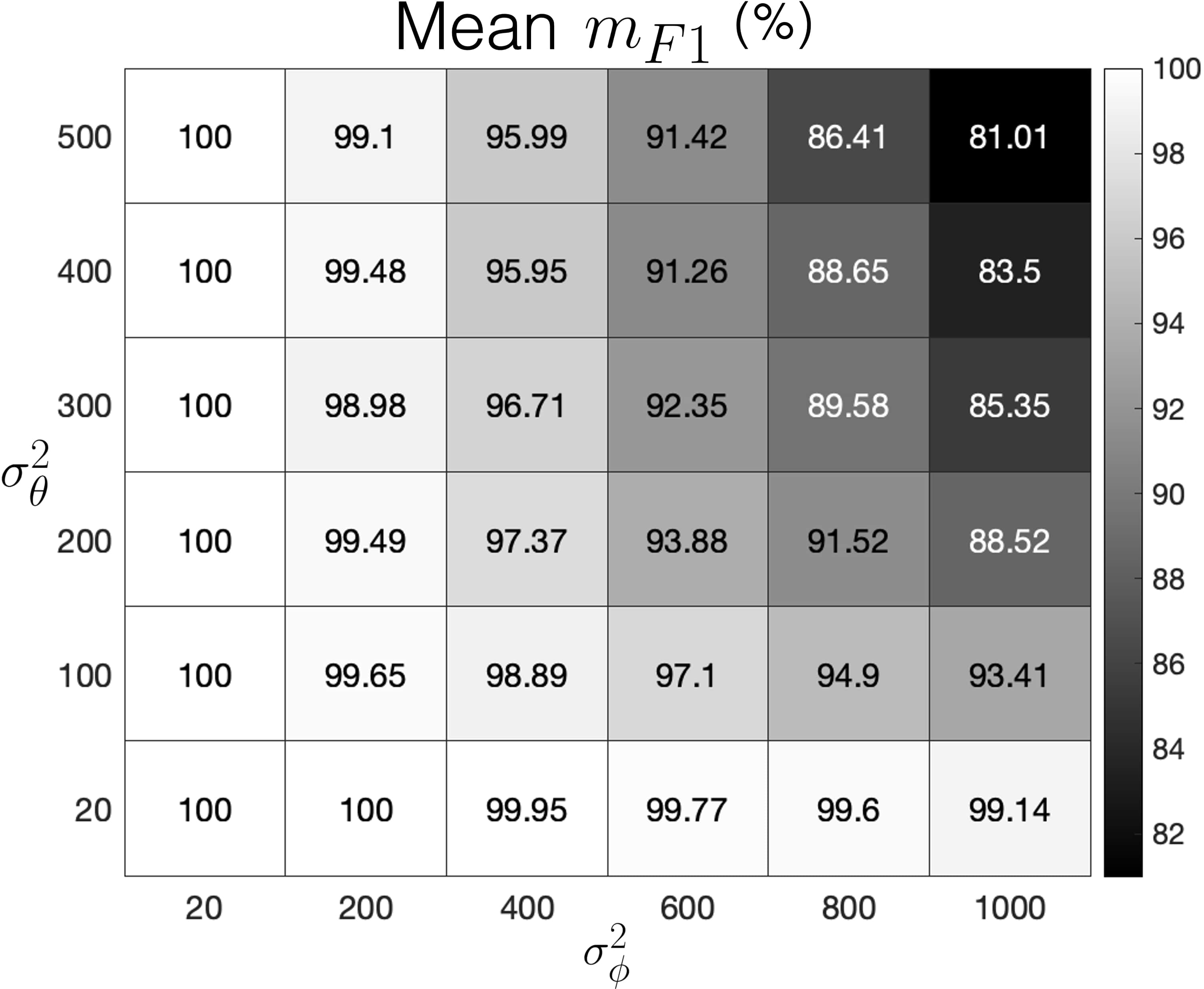
Fig. 10 shows the sleep posture classification performance given each augmentation setting in ${\bm{\Re}}$. Since all posture classes are equally weighted in $\prescript{{}_{\ooalign{\rule[3.01389pt]{3.01389pt}{0.4pt}\cr\hss\rule{0.4pt}{4.89998pt}\hss\cr}}}{}{\bm{\Psi}}^{v}({\bm{\tau}})$ and $\prescript{*}{}{\bm{\Psi}}^{v}({\bm{\tau}})$, we only show the mean and standard deviation of $m_{F1}$ as they are almost identical to that of $m_{acc}$. At the bottom left corner of ${\bm{\Re}}$ where the level of injected noise is lowest, $(\sigma_{\phi}^{2},\sigma_{\theta}^{2})=(20,20)$, a perfect $100\%$ $m_{F1}$ score with zero standard deviation is attained. On the opposite corner, where $(\sigma_{\phi}^{2},\sigma_{\theta}^{2})=(1000,500)$, exaggerated noise injection seems to pose more challenge to the classification task; nevertheless, the mean $m_{F1}$ remains above $81\%$ with small standard deviation.

The mean $m_{F1}$ heat map can be used to study the effect of each augmentation hyperparameter. When $\sigma_{\phi}^{2}$ is below $200$, the gradual increase of $\sigma_{\theta}^{2}$ barely affects the classification performance. On the other hand, the increase in $\sigma_{\phi}^{2}$ tend to have more influence over the performance when $\sigma_{\theta}^{2}$ is below $100$. As we move diagonally along ${\bm{\Re}}$ and near to the top right corner, the influence of stepping up $\sigma_{\theta}^{2}$ overtakes that of $\sigma_{\phi}^{2}$. Overall, the results obtained through the virtual experiment suggest that the proposed sleep posture learning framework is robust to mild-to-extreme variations in postural observations.

The participant study pipeline utilises one-shot learning only during the training phase, then validates the resultant trained model on “unseen” real timeseries. Therefore, some level of discrepancy (mismatch) is present between the augmented training dataset and test-labelled posture recordings. Therefore, the participant study complements the virtual experiment through exploring what data augmentation offers to sleep posture learning when unknown discrepancy exists between $\prescript{{}_{\ooalign{\rule[3.01389pt]{3.01389pt}{0.4pt}\cr\hss\rule{0.4pt}{4.89998pt}\hss\cr}}}{}{\bm{\Psi}}^{w}({\bm{\tau}})$ and $\prescript{*}{}{\bm{\Psi}}^{w}({\bm{t}})$.

Fig. 11 shows the results obtained via the proposed sleep posture learning framework. Owing to the class-imbalanced $\prescript{*}{}{\bm{\Psi}}^{w}({\bm{t}})$, both $m_{acc}$ and $m_{F1}$ scores are reported. It is evident that the data augmentation settings have a substantial influence over the classification performance, with $m_{F1}$ ranging roughly between $60\%\ \text{and}\ 90\%$. Given mild noise injection at $(\sigma_{\phi}^{2},\sigma_{\theta}^{2})=(20,20)$, the mean $m_{F1}$ score was found to be $72.2\%$.

Examining the $m_{F1}$ heat map of the human participant study provides a good picture of how augmentation hyperparameter tuning influences the classification performance. In the virtual experiment, each classifier was trained and tested on augmented observations sharing the same postural variability. For the participant study, different data augmentation settings are used to pre-train multiple classifier models that are later tested on the same testing posture dataset, $\prescript{*}{}{\bm{\Psi}}^{w}({\bm{t}})$, with unknown train-test pose discrepancy. Logically speaking, a good data augmentation setting would then be one that produces an augmented training posture dataset of variability level close to the actual train-test pose discrepancy. Based on this, recommendations for optimal tuning of the data augmentation hyperparameters can be informed.

To facilitate understanding, let us subdivide ${\bm{\Re}}$ in Fig. 11 into three subgrids annotated by , and to study the effect of different augmentation settings on the classification performance. Subgrid shows that angle-dominant augmentation yields performance metrics similar to that of $(\sigma_{\phi}^{2},\sigma_{\theta}^{2})=(20,20)$. For subgrid , the performance undergoes a falling trend ($m_{F1}$ as low as $60\%$) in response to augmenting the axes and angles of rotation simultaneously. Finally, subgrid showcases further performance enhancement brought by axis-dominant augmentation, boosting $m_{F1}$ to about $90\%$. The reason why augmenting axes is more useful may be related to the presence of environmental objects (e.g. mattress and pillow) which constrain joint rotations, hence, variation in sleep postures rather owes to deviations in joint axes of rotation. Consequently, subgrid is recommended for data augmentation, specifically given $\sigma_{\phi}^{2}\geqslant 800\cap\sigma_{\theta}^{2}=100$.

To further understand how axis-dominant augmentation can contribute up to $30\%$ gain in performance compared to other augmentation settings, we use UMAP-empowered data visualisation described in Section 4.5. Fig. 12 reports $\mathbfcal{U}$ for two different scenarios: mild noise injection at $(\sigma_{\phi}^{2},\sigma_{\theta}^{2})=(20,20)$ (Fig. 12(a)), and optimal axis-dominated augmentation at $(\sigma_{\phi}^{2},\sigma_{\theta}^{2})=(800,100)$ (Fig. 12(b)). At mild noise injection, Fig. 12(a) shows large discrepancies between training and testing observations across most sleep postures, as reflected by the sparse distribution of scattered clusters of observations. This clarifies why, in the absence of a sufficiently large dataset, it is hard to accomplish satisfactory posture classification performance. On the other hand, Fig. 12(b) showcases the effectiveness of the axis-dominant augmentation in bringing about structure to the data distribution as the training and testing observations of each posture are located in close proximity. The resultant classifier-friendly data distribution stands behind the significant rise in performance $(m_{acc}=92.7\%)$ and robustness to postural discrepancies compared to the mild augmentation case. Additionally, it is noteworthy how overlaps emerged between certain postures as in annotated regions , and .

The hybrid metric $\Lambda$ proposed in Section 4.5 can also be used to further understand the intra-posture similarities between: (i) $\mathbfcal{Y}_{1}\leftrightarrow\mathbfcal{Y}_{9}$, (ii) $\mathbfcal{Y}_{3}\leftrightarrow\mathbfcal{Y}_{12}$, and (iii) $\mathbfcal{Y}_{6}\leftrightarrow\mathbfcal{Y}_{10}$. Fig. 13 presents the mean $\Lambda$ with ${\bm{x}}_{a}$ and ${\bm{x}}_{b}$ exhausting all combinations of posture-specific (augmented) training and testing observations given the mild augmentation case $(\sigma_{\phi}^{2},\sigma_{\theta}^{2})=(20,20)$. Remarkably, the metric $\Lambda$ is capable of revealing postural similarities that UMAP did not capture in Fig. 12(a). Sifting data for such correlations and trends is of great significance to researchers and clinicians in terms of rethinking human postural analysis, for instance, to evaluate the efficacy of pose characterisation methods. Another possible usage of this map is the examination of posture definitions and confirming their parametric and subjective distinction from other postures before including it in the study.

Fig. 14(a) shows the confusion matrix given the optimal augmentation setting; $(\sigma_{\phi}^{2},\sigma_{\theta}^{2})=(800,100)$. The SVM-ECOC model achieves 100% classification accuracy on testing observations of all postures except $\mathbfcal{Y}_{5}$, demonstrating satisfactory robustness to the postural overlaps outlined in Figs. 12(b) and 13. Such overlaps were viewed as a challenge in similar studies although these works considered no more than eight postures of standard-to-moderate complexity, see for example [33]. To understand why the model confuses $\mathbfcal{Y}_{5}$ with $\mathbfcal{Y}_{7}$, we conduct a $\Lambda$-based similarity assessment specifically focused on the misclassification in Fig. 14(b). Since the model relies on augmented training data to handle unseen testing observations, we compare ${\bm{x}}_{a}=\prescript{*}{}{\tilde{\bm{x}}}_{5}(\bm{t}_{1\mathrel{\mathop{\mathchar 58\relax}}\Omega_{5}})$ against all ${\bm{x}}_{b}=\prescript{{}_{\ooalign{\rule[3.01389pt]{3.01389pt}{0.4pt}\cr\hss\rule{0.4pt}{4.89998pt}\hss\cr}}}{}{\tilde{\bm{x}}}_{j}(\bm{\tau})\ \forall j\in\left[1,12\right]$, where $\tilde{(\cdot)}$ denotes the mean in time domain. Fig. 14(b) reveals a small difference in $\Lambda$ between $\mathbfcal{Y}_{5}$ and $\mathbfcal{Y}_{7}$. Moreover, $\Lambda$ scores of both $\mathbfcal{Y}_{5}$ and $\mathbfcal{Y}_{7}$ indicate a moderate similarity level only around $6.5$ out of $8.0$, with no clear winner. Recalling region from Fig. 12(b), the relatively large train-to-test distance for $\mathbfcal{Y}_{5}$ confirms the participant was (unintentionally) inconsistent in replicating that posture during data collection, which again explains the misclassification of $\prescript{*}{}{\bm{x}}_{5}(\bm{t})$. Further inspection into the root cause of such discrepancy is presented in Fig. 15 which shows that the participant’s $\mathbfcal{J}(2)$ mean orientation differed considerably between train- and test-labelled recordings of $\mathbfcal{Y}_{5}$. Such inexact posture recreation by participants is an occasional challenge inherent to similar works, as in [32].

For the sake of comparison, Fig. 14(c) shows the result of the same assessment of Fig. 14(b) but with ${\bm{x}}_{a}=\prescript{*}{}{\tilde{\bm{x}}}_{7}(\bm{t}_{1\mathrel{\mathop{\mathchar 58\relax}}\Omega_{7}})$. Fig. 14(c) reveals an uncertainty-free scenario where $\mathbfcal{Y}_{7}$ has a similarity metric of about $7.9$ out of $8.0$. Therefore, the $\Lambda$ metric can be regarded as a confidence measure associated with the output posture label, indicating how far one can trust the system at any instant of time.

Interestingly, Figs. 14(b) and 14(c) shows that $\Lambda_{\phi}$ experience more acute variations in comparison to $\Lambda_{\theta}$. This clarifies why axis-dominant augmentation accomplishes better enhancement to the performance compared to angle-dominant augmentation. Such observation also reflects on the nature of in-bed postural analysis as environmental constraints essentially inhibit the mobility of joints, causing variation to mostly take place along the axial component.

For reference, posture classification using only the real training data available was conducted to directly evaluate the simulation-to-real (Sim2Real) gap. In this case, the training of the classification model is not limited to only one observation per posture (one shot). Instead, the SVM-ECOC model leverages the whole length of train-labelled posture recordings and utilises all observed segment-to-segment orientations for posture modelling. After 10 repeated train-test runs, the average classification accuracy of the model on $\prescript{*}{}{\bm{\Psi}}^{w}({\bm{t}})$ was found to be around $48.1\%$. The macro-averaged $m_{F1}$ is found to be $40.1\%$, which means the Sim2Real gap is $40\%$ to $60\%$. This chance-level accuracy reveals poor generalisation performance and justifies the need for a posture learning framework that better deals with data insufficiency - the aim of this paper. The proposed framework indeed provides a boost in $m_{F1}$ by more than 20% out of the box and before fine-tuning the data augmentation hyperparameters.

To the best knowledge of the authors, the presented work serves as the most advanced sleep posture analysis in the literature with twelve complex postures representing non-standard postural variations common during sleep. Similar works only covered no more than eight postures, many of which are minor variations of the four standard sleep postures. The protocol of sleep data collection is another crucial aspect that sets the presented methodology apart from others reported in the literature. Specifically, randomised strategies for both pose shuffling and train/test trial assignment are adopted to ensure statistical independence and to account for the participant gaining familiarity with the experiment over time. Moreover, the proposed one-shot posture learning framework makes the use of wearable technologies far easier and more viable, as it removes the need for expensive training data collection sessions. Lastly, the exclusive use of inertial sensor fusion brings forward approximate segment orientations instead of the rudimentary raw data approach often adopted in the literature. Therefore, our approach provides a more comprehensible posture representation to non-technical experts such as clinicians. To better highlight the benefits of the framework proposed in this paper, a comparison with existing works is summarised in Table 1.

Some state-of-the-art studies [32, 33] had reported the possible occurrence of intra-posture similarity and inexact posture recreation, and regarded these as limitations without a clear attempt of formally verifying or quantifying them. A distinctive highlight of this work is the proposed interpretation approaches which provide qualitative and quantitative insights into the nature of sleep postures, their augmentation, and the classification problem as a whole. Our investigation shows that appropriate augmentation settings can make the classification robust to intra-posture similarity.

References

- [1] A. Cieza, K. Causey, K. Kamenov, S. W. Hanson, S. Chatterji, T. Vos, Global estimates of the need for rehabilitation based on the global burden of disease study 2019: a systematic analysis for the global burden of disease study 2019, The Lancet 396 (2020) 2006–2017. doi:10.1016/S0140-6736(20)32340-0.
- [2] D. of Health) (Institution/Organization, The musculoskeletal services framework – a joint responsibilty: doing it differently (2006).
- [3] P. M. Clark, B. M. Ellis, A public health approach to musculoskeletal health (2014). doi:10.1016/j.berh.2014.10.002.
- [4] J. Hartvigsen, M. J. Hancock, A. Kongsted, Q. Louw, M. L. Ferreira, S. Genevay, D. Hoy, J. Karppinen, G. Pransky, J. Sieper, R. J. Smeets, M. Underwood, R. Buchbinder, D. Cherkin, N. E. Foster, C. G. Maher, M. van Tulder, J. R. Anema, R. Chou, S. P. Cohen, L. M. Costa, P. Croft, P. H. Ferreira, J. M. Fritz, D. P. Gross, B. W. Koes, B. Öberg, W. C. Peul, M. Schoene, J. A. Turner, A. Woolf, What low back pain is and why we need to pay attention, The Lancet 391 (2018) 2356–2367. doi:10.1016/S0140-6736(18)30480-X.
- [5] M. Abdel-Basset, W. Ding, L. Abdel-Fatah, The fusion of internet of intelligent things (ioit) in remote diagnosis of obstructive sleep apnea: A survey and a new model, Information Fusion 61 (2020) 84–100. doi:10.1016/j.inffus.2020.03.010.
- [6] L. Paquay, R. Wouters, T. Defloor, F. Buntinx, R. Debaillie, L. Geys, Adherence to pressure ulcer prevention guidelines in home care: A survey of current practice, Journal of Clinical Nursing 17 (2008) 627–636. doi:10.1111/j.1365-2702.2007.02109.x.
- [7] V. Ibáñez, J. Silva, O. Cauli, A survey on sleep questionnaires and diaries, Sleep Medicine 42 (2018) 90–96. doi:10.1016/j.sleep.2017.08.026.
- [8] G. D. Pinna, E. Robbi, M. T. L. Rovere, A. E. Taurino, C. Bruschi, G. Guazzotti, R. Maestri, Differential impact of body position on the severity of disordered breathing in heart failure patients with obstructive vs. central sleep apnoea, European Journal of Heart Failure 17 (2015) 1302–1309. doi:10.1002/ejhf.410.
- [9] W. H. Akeson, D. Amiel, M. F. Abel, S. R. Garfin, S. L. Woo, Effects of immobilization on joints, Clinical Orthopaedics and Related Research 219 (1987) 28–37. doi:10.1097/00003086-198706000-00006.
- [10] L. Parisi, F. Pierelli, G. Amabile, G. Valente, E. Calandriello, F. Fattapposta, P. Rossi, M. Serrao, Muscular cramps: Proposals for a new classification, Acta Neurologica Scandinavica 107 (2003) 176–186. doi:10.1034/j.1600-0404.2003.01289.x.
- [11] S. Akbarian, G. Delfi, K. Zhu, A. Yadollahi, B. Taati, Automated non-contact detection of head and body positions during sleep, IEEE Access 7 (2019) 72826–72834. doi:10.1109/ACCESS.2019.2920025.
- [12] Y. Y. Li, Y. J. Lei, L. C. L. Chen, Y. P. Hung, Sleep posture classification with multi-stream cnn using vertical distance map, International Workshop on Advanced Image Technology (IWAIT) (2018) 1–4. doi:10.1109/IWAIT.2018.8369761.
- [13] S. M. Mohammadi, M. Alnowami, S. Khan, D. J. Dijk, A. Hilton, K. Wells, Sleep posture classification using a convolutional neural network, 40th Annual International Conference of the IEEE Engineering in Medicine and Biology Society (EMBC) (2018) 1–4. doi:10.1109/EMBC.2018.8513009.
- [14] T. H. Kim, S. J. Kwon, H. M. Choi, Y. S. Hong, Determination of lying posture through recognition of multitier body parts, Wireless Communications and Mobile Computing 2019 (2019) 1–16. doi:10.1155/2019/9568584.
- [15] M. Alaziz, Z. Jia, R. Howard, X. Lin, Y. Zhang, In-bed body motion detection and classification system, ACM Transactions on Sensor Networks 16 (2020) 13:1–13–26. doi:https://doi.org/10.1145/3372023.
- [16] U. Qureshi, F. Golnaraghi, An algorithm for the in-field calibration of a mems imu, IEEE Sensors Journal 17 (2017) 7479– 7486. doi:10.1109/JSEN.2017.2751572.
- [17] B. Fan, Q. Li, T. Tan, P. Kang, P. B. Shull, Effects of imu sensor-to-segment misalignment and orientation error on 3-d knee joint angle estimation, IEEE Sensors Journal 22 (2022) 2543–2552. doi:10.1109/JSEN.2021.3137305.
- [18] A. Leardini, A. Chiari, U. D. Croce, A. Cappozzo, Human movement analysis using stereophotogrammetry part 3. soft tissue artifact assessment and compensation, Gait and Posture 21 (2005) 212–225. doi:10.1016/j.gaitpost.2004.05.002.
- [19] B. V. Vaughn, P. Giallanza, Technical review of polysomnography, Chest 134 (2008) 1310–1319. doi:10.1378/chest.08-0812.
- [20] L. C. Markun, A. Sampat, Clinician-focused overview and developments in polysomnography, Current Sleep Medicine Reports 6 (2020) 309–321. doi:10.1007/s40675-020-00197-5.
- [21] H. R. Colten, B. M. Altevogt, Sleep disorders and sleep deprivation: An unmet public health problem, 2006. doi:10.17226/11617.
-
[22]
A. Tiotiu, O. Mairesse, G. Hoffmann, D. Todea, A. Noseda,
Body position and breathing
abnormalities during sleep: A systematic study, Pneumologia 60 (2011)
216–221.
URL https://europepmc.org/article/med/22420172 - [23] J. Verbraecken, Applications of evolving technologies in sleep medicine, Breathe 9 (2013) 442–455. doi:10.1183/20734735.012213.
- [24] J. Razjouyan, H. Lee, S. Parthasarathy, J. Mohler, A. Sharafkhaneh, B. Najafi, Information from postural/sleep position changes and body acceleration: A comparison of chest-worn sensors, wrist actigraphy, and polysomnography, Journal of Clinical Sleep Medicine 13 (2017) 1301–1310. doi:10.5664/jcsm.6802.
- [25] I. H. Lopez-Nava, M. M. Angelica, Wearable inertial sensors for human motion analysis: A review, IEEE Sensors Journal 16 (2016) 7821–7834. doi:10.1109/JSEN.2016.2609392.
- [26] Z. Zhang, G. Z. Yang, Monitoring cardio-respiratory and posture movements during sleep: What can be achieved by a single motion sensor, IEEE 12th International Conference on Wearable and Implantable Body Sensor Networks (BSN) (2015) 1–6. doi:10.1109/BSN.2015.7299409.
- [27] X. Sun, L. Qiu, Y. Wu, Y. Tang, G. Cao, Sleepmonitor: Monitoring respiratory rate and body position during sleep using smartwatch, Proceedings of the ACM on Interactive, Mobile, Wearable and Ubiquitous Technologies 1 (2017) 1–22. doi:10.1145/3130969.
- [28] O. S. Eyobu, Y. W. Kim, D. Cha, D. S. Han, A real-time sleeping position recognition system using imu sensor motion data, IEEE International Conference on Consumer Electronics (ICCE) 2018-Janua (2018) 1–2. doi:10.1109/ICCE.2018.8326209.
- [29] P. Alinia, A. Samadani, M. Milosevic, H. Ghasemzadeh, S. Parvaneh, Pervasive lying posture tracking, Sensors (Switzerland) 20 (2020) 1–22. doi:10.3390/s20205953.
- [30] S. Jeon, T. Park, A. Paul, Y. S. Lee, S. H. Son, A wearable sleep position tracking system based on dynamic state transition framework, IEEE Access 7 (2019) 135742–135756. doi:10.1109/ACCESS.2019.2942608.
- [31] E. B. Monroy, A. P. Rodríguez, M. E. Estevez, J. M. Quero, Fuzzy monitoring of in-bed postural changes for the prevention of pressure ulcers using inertial sensors attached to clothing, Journal of Biomedical Informatics 107 (2020) 1–12. doi:10.1016/j.jbi.2020.103476.
- [32] R. M. Kwasnicki, G. W. Cross, L. Geoghegan, Z. Zhang, P. Reilly, A. Darzi, G. Z. Yang, R. Emery, A lightweight sensing platform for monitoring sleep quality and posture: A simulated validation study, European Journal of Medical Research 23 (2018) 1–9. doi:10.1186/s40001-018-0326-9.
- [33] S. Fallmann, R. V. Veen, L. Chen, D. Walker, F. Chen, C. Pan, Wearable accelerometer based extended sleep position recognition, IEEE 19th International Conference on e-Health Networking, Applications and Services (Healthcom) (2017) 1–6. doi:10.1109/HealthCom.2017.8210806.
- [34] O. Elnaggar, F. Coenen, P. Paoletti, In-bed human pose classification using sparse inertial signals, Lecture Notes in Computer Science (including subseries Lecture Notes in Artificial Intelligence and Lecture Notes in Bioinformatics) 12498 LNAI (2020) 331–344. doi:10.1007/978-3-030-63799-6_25.
- [35] L. Chang, J. Lu, J. Wang, X. Chen, D. Fang, Z. Tang, P. Nurmi, Z. Wang, Sleepguard: Capturing rich sleep information using smartwatch sensing data, Proceedings of the ACM on Interactive, Mobile, Wearable and Ubiquitous Technologies 2 (2018) 1–34. doi:10.1145/3264908.
- [36] M. Airaksinen, O. Räsänen, E. Ilén, T. Häyrinen, A. Kivi, V. Marchi, A. Gallen, S. Blom, A. Varhe, N. Kaartinen, L. Haataja, S. Vanhatalo, Automatic posture and movement tracking of infants with wearable movement sensors, Scientific Reports 10 (2020) 1–12. doi:10.1038/s41598-019-56862-5.
- [37] H. Ohashi, M. Al-Naser, S. Ahmed, K. Nakamura, T. Sato, A. Dengel, Attributes’ importance for zero-shot pose-classification based on wearable sensors, Sensors 18 (2018) 1–17. doi:10.3390/s18082485.
- [38] A. Mobasheri, M. Batt, An update on the pathophysiology of osteoarthritis, Annals of Physical and Rehabilitation Medicine 59 (2016) 333–339. doi:10.1016/j.rehab.2016.07.004.
- [39] S. J. McCabe, A. L. Uebele, V. Pihur, R. S. Rosales, I. Atroshi, Epidemiologic associations of carpal tunnel syndrome and sleep position: Is there a case for causation?, Hand 2 (2007) 127–134. doi:10.1007/s11552-007-9035-5.
- [40] S. O. Madgwick, A. J. Harrison, R. Vaidyanathan, Estimation of imu and marg orientation using a gradient descent algorithm, Proceedings of the IEEE International Conference on Rehabilitation Robotics (2011) 179–185doi:10.1109/ICORR.2011.5975346.
- [41] X. Xiao, S. Zarar, Machine learning for placement-insensitive inertial motion capture, IEEE International Conference on Robotics and Automation (ICRA) (2018) 6716–6721. doi:10.1109/ICRA.2018.8463176.
- [42] M. Nazarahari, H. Rouhani, Semi-automatic sensor-to-body calibration of inertial sensors on lower limb using gait recording, IEEE Sensors Journal 19 (2019) 12465– 12474. doi:10.1109/JSEN.2019.2939981.
- [43] T. Zimmermann, B. Taetz, G. Bleser, Imu-to-segment assignment and orientation alignment for the lower body using deep learning, Sensors 18 (2018) 1–35. doi:10.3390/s18010302.
[44]
M. Olson, A. J. Wyner, R. Berk,
Modern
neural networks generalize on small data sets, Advances in Neural
Information Processing Systems (2018) 3619–3628.
URL https://papers.nips.cc/paper/2018/hash/fface8385abbf94b4593a0ed53a0c70f-Abstract.html - [45] R. Blagus, L. Lusa, Smote for high-dimensional class-imbalanced data, BMC Bioinformatics 14 (2013) 1–16. doi:10.1186/1471-2105-14-106.
- [46] C. Shorten, T. M. Khoshgoftaar, A survey on image data augmentation for deep learning, Journal of Big Data 6 (2019) 1–48. doi:10.1186/s40537-019-0197-0.
- [47] Q. Wen, L. Sun, F. Yang, X. Song, J. Gao, X. Wang, H. Xu, Time series data augmentation for deep learning: A survey, Proceedings of the Thirtieth International Joint Conference on Artificial Intelligence (2021) 4653–4660. doi:10.24963/ijcai.2021/631.
- [48] B. K. Iwana, S. Uchida, An empirical survey of data augmentation for time series classification with neural networks, PLoS ONE 16. doi:10.1371/journal.pone.0254841.
- [49] K. M. Rashid, J. Louis, Window-warping: A time series data augmentation of imu data for construction equipment activity identification, Proceedings of the 36th International Symposium on Automation and Robotics in Construction (ISARC) (2019) 651–657. doi:10.22260/isarc2019/0087.
- [50] M. Arslan, M. Guzel, M. Demirci, S. Ozdemir, Smote and gaussian noise based sensor data augmentation, Proceedings of the 4th International Conference on Computer Science and Engineering (UBMK) (2019) 458–462. doi:10.1109/UBMK.2019.8907003.
- [51] T. G. Dietterich, G. Bakiri, Solving multiclass learning problems via error-correcting output codes, Journal of Artificial Intelligence Research 2 (1995) 263–286. doi:10.1613/jair.105.
- [52] E. L. Allwein, R. E. Schapire, Y. Singer, Reducing multiclass to binary: A unifying approach for margin classifiers, Journal of Machine Learning Research 1 (2001) 113–141. doi:10.1162/15324430152733133.
- [53] C. W. Hsu, C. J. Lin, A comparison of methods for multiclass support vector machines, IEEE Transactions on Neural Networks 13 (2002) 415–425. doi:10.1109/72.991427.
- [54] S. Escalera, O. Pujol, P. Radeva, On the decoding process in ternary error-correcting output codes, IEEE Transactions on Pattern Analysis and Machine Intelligence 32 (2010) 120–134. doi:10.1109/TPAMI.2008.266.
- [55] S. Abe, Chapter 2: Two-class support vector machines (2010). doi:10.1007/978-1-84996-098-4_2.
- [56] B. Shahriari, K. Swersky, Z. Wang, R. P. Adams, N. D. Freitas, Taking the human out of the loop: A review of bayesian optimization, Proceedings of the IEEE 104 (2016) 148–175. doi:10.1109/JPROC.2015.2494218.
[57]
O. J. Woodman,
An
introduction to inertial navigation (report no. ucam-cl-tr-696) (2007).
URL https://www.cl.cam.ac.uk/techreports/UCAM-CL-TR-696.pdf - [58] M. Kok, J. D. Hol, T. B. Schön, Using inertial sensors for position and orientation estimation, Foundations and Trends in Signal Processing 11. doi:10.1561/2000000094.
- [59] H. He, Y. Ma, Imbalanced learning: Foundations, algorithms, and applications, 2013. doi:10.1002/9781118646106.
- [60] L. McInnes, J. Healy, J. Melville, Umap: Uniform manifold approximation and projection for dimension reduction, arXiv preprint (2018) 1–63. doi:10.48550/arXiv.1802.03426.
- [61] O. Elnaggar, R. Arelhi, Quantification of knowledge exchange within classrooms: An ai-based approach, The European Conference on Education 2021: Official Conference Proceedings (2021) 1–11. doi:10.22492/issn.2188-1162.2021.17.
- [62] O. Elnaggar, R. Arelhi, A new unsupervised short-utterance based speaker identification approach with parametric t-sne dimensionality reduction, International Conference on Artificial Intelligence in Information and Communication (ICAIIC) (2019) 1–10. doi:10.1109/ICAIIC.2019.8669051.
[63]
C. Meehan, J. Ebrahimian, W. Moore, S. Meehan,
Uniform
manifold approximation and projection (umap), MATLAB Central File Exchange.
URL https://www.mathworks.com/matlabcentral/fileexchange/71902 - [64] B. Taetz, G. Bleser, M. Miezal, Towards self-calibrating inertial body motion capture, Proceedings of the 19th International Conference on Information Fusion (FUSION) (2016) 1751–1759. doi:10.48550/arXiv.1606.03754.
- [65] J. Solà, Quaternion kinematics for the error-state kalman filter, arXiv preprint (2017) 1–95. doi:10.48550/arXiv.1711.02508.
- [66] E. Kraft, A quaternion-based unscented kalman filter for orientation tracking, Proceedings of the 6th International Conference on Information Fusion (FUSION) 1 (2003) 47–54. doi:10.1109/ICIF.2003.177425.