Singularity formation for the general Poiseuille flow of nematic liquid crystals
Abstract.
We consider the Poiseuille flow of nematic liquid crystals via the full Ericksen-Leslie model. The model is described by a coupled system consisting of a heat equation and a quasilinear wave equation. In this paper, we will construct an example with a finite time cusp singularity due to the quasilinearity of the wave equation, extended from an earlier result on a special case.
1 Department of Mathematics, University of Kansas, Lawrence, KS 66045, U.S.A.
Email: [email protected],
2 Department of Mathematics, University of Kansas, Lawrence, KS 66045, U.S.A. Email: [email protected].
Dedicated to Professor Tong Zhang in the occasion of his 90-th birthday.
1. Introduction:
The state of a nematic liquid crystal is characterized by its velocity field for the flow and its director field for the alignment of the rod-like feature. These two characteristics interact with each other so that any distortion of the director causes a motion and, likewise, any flow affects the alignment . One famous model on nematic liquid crystal is the Ericksen-Leslie model for nematics that was first proposed by Ericksen [11] and Leslie [15] in the 1960’s.
In this paper, we consider the Poiseulle flow via the full Ericksen-Leslie model, when and take the form
where and the motion is along the -axis and the director lies in the -plane with angle made from the -axis. Then the Ericksen-Leslie system can be written as
| (1.1) | ||||
| (1.2) |
where the functions and are explicitly given by
| (1.3) | ||||
Here, , are positive elastic constants in the Oseen-Frank energy. The material coefficients and reflect the molecular shape and the slippery part between fluid and particles. The coefficients and coefficients , satisfy the following physical relations:
| (1.4) |
The first two relations are compatibility conditions, while the third relation is called Parodi’s relation, derived from Onsager reciprocal relations expressing the equality of certain relations between flows and forces in thermodynamic systems out of equilibrium (cf. [17]). The coefficients also satisfy the following empirical relations (p.13, [16])
| (1.5) | ||||
A detailed derivation of the Ericksen-Leslie system for Poiseulle flows can be found in [7], where without loss of generality, we choose density to be , and the inertial coefficient of the director to be . Furthermore, for simplicity, the constant in the model in [7], which is the gradient of pressure along the flow direction, is set to be zero.
Due to the quasilinearity of the wave equation on , finite time gradient blowup might happen even when the initial data are smooth. In [7], Chen, Huang and Liu established an example showing such kind of singularity formation phenomena, for a special case of (1.1)-(1.2) when and .
The construction of the singularity formation example relies on the framework in [13] by Glassy-Hunter-Zheng on the variational wave equation
| (1.6) |
The global well-posedness theories of Hölder continuous solutions for variational wave equations and systems related to nematic liquid crystals have been intensively studied in the last two decades [1, 2, 3, 4, 5, 6, 9, 10, 14, 18, 19, 20].
The proof of finite time singularity formation in [7] for the special case of (1.1)-(1.2) also relies on a crucial estimate on the bound of a new function , where in the general case,
| (1.7) |
We note that functions and both blow up when singularity forms, however, their combination will be proved uniformly bounded. This estimate, first obtained in [7] for the special case (when and ), is crucial for both singularity formation and global existence of Hölder continuous solution for the system (1.1)-(1.2).
Using (1.7), the wave equation (1.2) can be written as
| (1.8) |
From (1.3)-(1.5), we have the following bounds for , and
| (1.9) | ||||
where and are constants such that and are strictly positive. Furthermore, physical laws in (1.4) and (1.5) give that
| (1.10) |
for some positive constant , where the proof can be found in [7].
In this paper, we will first find a bound on in terms of the initial energy. So (1.8) is a damped variational wave equation adding a uniform bounded source term . Then we can prove the singularity formation of cusp singularity using the methods in [13, 10, 7]. Note the source term in the original equation (1.2) may be unbounded.
In another companion paper [8], we will show that is bounded under the norm of for some positive constant , even for weak solutions including singularities. This is one of the key estimates for the global existence proof.
Except showing one example forming the cusp singularity, another motivation of this paper is to introduce the major mathematical idea why we can get better regularity on than or , in the general case. For smooth solutions, we can explain the idea in a relatively easier manner than for weak solutions.
Now, let’s expain the main difficulty in controlling for the general case comparing to the special case. For the special case considered in [7] (when and ), (1.1) is
so can be solved directly by . However, this is not true for the general case. The main difficulty we need to overcome is the varying coefficient in the heat equation (1.1). Although is strictly positive and uniformly bounded, it is only Hölder continuous on and at the blowup. Therefore, the derivatives of on and blow up when singularity forms. This creates a lot of essential problems for finding a uniform bound on , since we need to use both heat and wave equations to bound . One of our key ideas is to consider the potential of , with .
Before we state the main result we define the following function with , that is used to design the initial data. Take with
| (1.11) |
| (1.12) |
and
| (1.13) |
where is a constant such that and are some positive constants.
Here is the main singularity formation result.
Theorem 1.
Let the initial data be
| (1.14) |
and
where is a constant such that , and is a function satisfying
| (1.15) |
and such that is a function. Then there exists a sufficiently small positive choice of the parameter such that the solution of (1.1)-(1.2) is only up to a finite time. More precisely, the solution is continuously differentiable up to some time before
In the proof of the theorem we will show that the singularity happens in the following form: there exists a time such that
| (1.16) |
as along the characteristic having the blowup phenomena. In this example, the initial energy is small, and initial data are smooth, but finite time singularity still forms. The singularity is a cusp type of singularity, combining with the existence result in [8], also see [7, 13].
The rest of the paper is divided into 3 sections as follows. In Section 2 we show the decay of the energy associated with a smooth solution. Section 3 contains the main estimate on the quantity : we show the uniform bound of over a fixed time interval. In Section 4, we prove the singularity formation result in Theorem 1.
2. The energy of the system
The energy of the system (1.1)-(1.2) is defined as
| (2.1) |
In this section we show the energy decay for smooth solutions.
Proposition 2.1.
Proof.
Therefore, considering only smooth solutions, for any , we have
| (2.5) |
3. Uniform bound on in finite time
For convenience, we just fix and give a uniform upper bound on , defined in (1.7), when , when solution is smooth. In fact, one can choose to be any positive constant, and still prove that is bounded.
Before our calculation, we recall the bounds in (1.9) and (1.10), and also note that and are bounded above by a constant because of (1.3).
3.1. An integral relation on and its estimate
We study the potential of , defined as
So
In terms of the quantity we can write the system as
| (3.1) | ||||
| (3.2) |
And we derive the following equation for .
Integrating it by parts, we get
| (3.3) |
In summary we consider the following Cauchy problem
| (3.4) |
where
with
| (3.5) |
It is easy to verify that, there exists some positive constant , such that
| (3.6) |
In this section, without confusion, we always use to denote different positive constants for different estimates.
Now using the conclusion from Chapter 1, Theorem 12 in [12], we can formally solve by (3.4) as
| (3.7) |
where the kernel can be written in terms of the heat kernel as follows,
| (3.8) |
where
| (3.9) |
The function is determined by the condition
where
It can be shown that such function exists and
| (3.10) |
where is a constant depending on Moreover, we have the following bounds for and
| (3.11) |
| (3.12) |
The reader can find the proof of the above estimates in Chapter 1, Theorem 11 in [12].
Now, differentiating (3.1) w.r.t we obtain that satisfies the following relation
| (3.13) |
Then we use this expression to find the uniform upper bound on . First, we give uniform bounds on , and in terms of , and the initial energy.
3.2. estimates on and
3.3. estimates on
Lemma 3.1.
Let be such that we have
| (3.17) | ||||
| (3.18) |
for some constants and .
Proof.
Recall:
| (3.19) |
and
| (3.20) |
Also note that due to the dependence of on we have the following relation
| (3.21) |
Starting with the first term of and using the above relation, there are three integrals to estimate. The integral related to the first term in (3.21) is
| (3.22) |
We have
| (3.23) |
The integral related to the second term of (3.21) can be easily estimated as
| (3.24) |
The integral related to the third term of (3.21) has a similar bound as the second term, using the change of variable
Combing above estimates, we obtain the following estimate
| (3.25) |
For the term with (the second term in (3.19)) we have:
Combining this estimate and (3.25), we prove the lemma. ∎
3.4. Uniform bound on
4. Singularity formation for classical solutions:
In this section we prove Theorem 1. For reader’s convenience, we recall the system
| (4.1) | ||||
| (4.2) |
and the initial data
| (4.3) | ||||
| (4.4) |
where is a function satisfying
| (4.5) |
and the function satisfies
| (4.6) |
| (4.7) |
and
| (4.8) |
Here is a constant such that and is some constant.
Remark 4.1.
A choice of the function can be a cubic polynomial constructed by satisfying the following constraints,
Some calculations lead to
The derivative is a quadratic polynomial that vanishes at the end points and The parabola is either concave or convex depending on the sign of the integral In any case, the critical point of the derivative is
This means
Now we define the following gradient variables representing the rate of change of along the forward and backward characteristics:
Direct calculations give:
| (4.9) |
| (4.10) |
and the following balance laws,
| (4.11) |
| (4.12) |
So we can get the following equation
| (4.13) |
with the initial conditions
| (4.14) |
Under the help of energy decay we obtain
| (4.16) |
Hence, by (3.29), it is easy to get that
| (4.17) |
where we use (3.29), (4.16) and
Furthermore, is small enough such that (3.27) is satisfied.
)
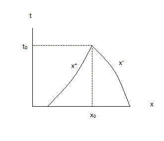
Now, we consider the two characteristic curves given by
with and See figure 1. Since the wave speed has a positive lower bound, two characteristics intersect at some point, say so we have and
| (4.18) |
We assume that . We will verify it later by showing that blowup will happen before .
Integrating (4.13) over the triangle (see figure 1), and applying the divergence theorem, then we have
| (4.19) |
Rearranging it, we have
By the decay of energy and , we obtain
| (4.20) |
Similarly, by the decay of energy, , and also using (4.17) and (4.18), we have
So we have
Next we consider a forward characteristic that we denote by
for , such that
Integrating the equation
we obtain
Using the smoothness of , when is small enough,
Next, we claim that for smooth solutions we have as long as To prove it by an contradiction argument, we assume that for some time in the interval. Define
By the continuity of we have
Define
Some calculations give
This means along the curve for
| (4.21) |
Dividing it by then integrating it over , we have
Recalling we have
| (4.22) |
for some positive constant .
For small enough,
then
Hence
which gives This is a contradiction with the definition of
This proves that as long as
Now using same calculations, we obtain
As a consequence, blows up before
Now choose small enough, we know the solution will blowup before
More precisely, there exists a time such that
as This shows that or as
On the other hand, because of the smallness of initially, i.e. is of order and (4.10), we know that remains uniformly bounded before the blowup of This shows that both
simultaneously as , at the blowup point.
This completes the proof of Theorem 1.
Acknowledgments
The authors are partially supported by NSF grant DMS-2008504. This paper is motivated by a discussion with Weishi Liu. The authors thank Weishi Liu for the helpful comments.
Conflict of interest statement
On behalf of all authors, the corresponding author states that there is no conflict of interest.
References
- [1] A. Bressan and G. Chen, Lipschitz metric for a class of nonlinear wave equations. Arch. Ration. Mech. Anal. 226 (2017), no. 3, 1303-1343.
- [2] A. Bressan and G. Chen, Generic regularity of conservative solutions to a nonlinear wave equation. Ann. I. H. Poincaré–AN 34 (2017), no. 2, 335-354.
- [3] A. Bressan, G. Chen, and Q. Zhang, Unique conservative solutions to a variational wave equation. Arch. Ration. Mech. Anal. 217 (2015), no. 3, 1069-1101.
- [4] A. Bressan and T. Huang Representation of dissipative solutions to a nonlinear variational wave equation. Comm. Math. Sci. 14 (2016), 31-53.
- [5] A. Bressan and Y. Zheng, Conservative solutions to a nonlinear variational wave equation. Comm. Math. Phys. 266 (2006), 471-497.
- [6] H. Cai, G. Chen, and Y. Du, Uniqueness and regularity of conservative solution to a wave system modeling nematic liquid crystal. J. Math. Pures Appl. 9 (2018), no 117, 185-220.
- [7] G. Chen, T. Huang and W. Liu, Poiseuille Flow of Nematic Liquid Crystals via the Full Ericksen–Leslie Model. Archive for Rational Mechanics and Analysis. 236, 839–891 (2020).
- [8] G. Chen, M. Sofiani and W. Liu, Global existence of Hölder continuous solution for Poiseuille flow of nematic liquid crystals, submitted.
- [9] G. Chen, P. Zhang, and Y. Zheng, Energy Conservative Solutions to a Nonlinear Wave System of Nematic Liquid Crystals. Comm. Pure Appl. Anal. 12 (2013), no 3, 1445-1468.
- [10] G. Chen and Y. Zheng, Singularity and existence to a wave system of nematic liquid crystals. J. Math. Anal. Appl. 398 (2013), 170-188.
- [11] J. L. Ericksen, Hydrostatic theory of liquid crystals. Arch. Ration. Mech. Anal. 9 (1962), 371-378.
- [12] A. Friedman, Partial Differential Equations of Parabolic Type, Prentice-Hall, Inc., 1964.
- [13] R. T. Glassey, J. K. Hunter, and Y. Zheng, Singularities in a nonlinear variational wave equation. J. Differential Equations 129 (1996), 49-78.
- [14] H. Holden and X. Raynaud, Global semigroup of conservative solutions of the nonlinear variational wave equation. Arch. Ration. Mech. Anal. 201 (2011), 871-964.
- [15] F. M. Leslie, Some thermal effects in cholesteric liquid crystals. Proc. Roy. Soc. A. 307 (1968), 359-372.
- [16] F. M. Leslie, Theory of Flow Phenomena in Liquid Crystals. Advances in Liquid Crystals, Vol. 4, 1-81. Academic Press, New York, 1979.
- [17] O. Parodi, Stress tensor for a nematic liquid crystal. J. Phys. 31 (1970), 581–584.
- [18] P. Zhang and Y. Zheng, Weak solutions to a nonlinear variational wave equation. Arch. Ration. Mech. Anal. 166 (2003), 303–319.
- [19] P. Zhang and Y. Zheng, Conservative solutions to a system of variational wave equations of nematic liquid crystals. Arch. Ration. Mech. Anal. 195 (2010), 701-727.
- [20] P. Zhang and Y. Zheng, Energy conservative solutions to a one-dimensional full variational wave system. Comm. Pure Appl. Math. 55 (2012), 582-632.