Singular layer PINN methods for Burgers’ equation
Abstract.
In this article, we present a new learning method called sl-PINN to tackle the one-dimensional viscous Burgers problem at a small viscosity, which results in a singular interior layer. To address this issue, we first determine the corrector that characterizes the unique behavior of the viscous flow within the interior layers by means of asymptotic analysis. We then use these correctors to construct sl-PINN predictions for both stationary and moving interior layer cases of the viscous Burgers problem. Our numerical experiments demonstrate that sl-PINNs accurately predict the solution for low viscosity, notably reducing errors near the interior layer compared to traditional PINN methods. Our proposed method offers a comprehensive understanding of the behavior of the solution near the interior layer, aiding in capturing the robust part of the training solution.
Key words and phrases:
Singular perturbations, Physics-informed neural networks, Burgers’ equation, Interior layers2000 Mathematics Subject Classification:
76D05, 68T99, 65M99, 68U991. Introduction
We consider the 1D Burgers’ equation, particularly focusing on scenarios where the viscosity is small, resulting in the formation of interior layers,
| (1.1) |
where is the given initial data and is the small viscosity parameter. The Burgers’ equation (1.1) is supplemented with one of the following boundary conditions,
-
()
is periodic in , provided that the initial data in is periodic in as well;
-
()
as and as where the boundary data and are smooth functions in time.
In the examples presented in Section 4, we consider the case where the data , , and are sufficiently regular. Therefore, the Burgers’ equation at a fixed viscosity is well-posed up to any finite time and satisfies
| (1.2) |
for a constant depending on the data, but independent of the viscosity parameter ; see, e.g., [4] for the proof when the boundary condition () above is imposed.
The corresponding limit of at the vanishing viscosity satisfies the inviscid Burgers’ equation,
| (1.3) |
supplemented with () or () above as for the viscous problem (1.1). Concerning all the examples in Section 4, the limit solution exhibits a discontinuous interior shock located at , (either stationary or moving ), and is smooth on each side of . Hence by identifying the states of a shock, we introduce smooth one-side solutions,
| (1.4) |
Setting , the solution satisfies that
| (1.5) |
and, in addition, we have
| (1.6) |
Note that, in this case, the viscous solution is located between the left and right solutions of at the shock , i.e.,
| (1.7) |
The primary goal of this article is to analyze and approximate the solution of (1.1) as the viscosity tends to zero when the (at least piecewise) smooth initial data creates an interior shock of . Specifically, we introduce a new machine learning technique called a singular-layer Physics-Informed Neural Network (sl-PINN) to accurately predict solutions to (1.1) when the viscosity is small. Following the methodology outlined in [11, 10, 9, 8], in Section 2, we start by revisiting the asymptotic analysis for (1.1) as presented in [4]; see, e.g., [3, 12, 13, 23] as well. Then, utilizing the interior layer analysis, we proceed to build our new sl-PINNs for (1.1) in Sections 3. The numerical computations for our sl-PINNs, along with a comparison to those from conventional PINNs, are detailed in Section 4. Finally, in the conclusion in Section 5, we summarize that the predicted solutions via sl-PINNs approximate the stiff interior layer of the Burgers problem quite accurately.
2. Interior layer analysis
We briefly recall from [4] the interior layer analysis for (1.1) that is made useful in the section below 3 where we construct our singular-layer Physics-Informed Neural Networks (sl-PINNs) for Burgers’ equation. To analyze the interior layer of the viscous Burgers’ equation (1.1), we first introduce a moving coordinate in space, centered at the shock location ,
| (2.1) |
and write the solutions of (1.1) and (1.3) with respect to the new system in the form,
| (2.2) |
The initial condition is written in terms of the new coordinate as
| (2.3) |
Now we set
| (2.4) |
where and are the disjoint and smooth portions of located on the left-hand side and the right-hand side of the shock at , and they are defined by
| (2.5) |
Using (1.1) and (2.1), and applying the chain rule, one can verify that the and satisfy the equations below:
| (2.6) |
and
| (2.7) |
Thanks to the moving coordinate system , now we are ready to analyze the interior shock layer near by investigating the two disjoint boundary layers of and , located on the left-hand and right-hand sides of . To this end, we introduce asymptotic expansions in the form,
| (2.8) |
Here and are the disjoint and smooth portions of located on the left-hand side and the right-hand side of , given by
| (2.9) |
i.e., for each .
The or in the asymptotic expansion (2.8) is an artificial function, called the corrector, that approximates the stiff behavior of , , near the shock of at (or equivalently ). Following the asymptotic analysis in [4], we define the correctors and as the solutions of
| (2.10) |
and
| (2.11) |
where
| (2.12) |
Thanks to the property of , (1.2), we notice that the value of is bounded by a constant independent of the small viscosity parameter .
We recall from Lemma 3.1 in [4] that the explicit expression of (and hence of by the symmetry) is given by
| (2.13) |
where
The validity of our asymptotic expansion of in (2.4) and (2.8) as well as the vanishing viscosity limit of to are rigorously verified in [4], and here we briefly recall the result without providing the detailed and technical proof; see Theorem 3.5 in [4]:
Under a certain regularity condition on the limit solution and , the asymptotic expansion in (2.4) and (2.8) is valid in the sense that
| (2.14) |
for a generic constant depending on the data, but independent of the viscosity parameter . Moreover, the viscous solution converges to the corresponding limit solution as the viscosity vanishes in the sense that
| (2.15) |
for a constant depending on the data, but independent of .
3. PINNs and sl-PINNs for Burgers’ equation
In this section, we are developing a new machine learning process called the singular-layer Physics-Informed Neural Network (sl-PINN) for the Burgers’ equation (1.1). We will be comparing its performance with that of the usual PINNs, specifically when the viscosity is small and hence the viscous Burgers’ solution shows rapid changes in a small region known as the interior layer. To start, we provide a brief overview of Physics-Informed Neural Networks (PINNs) for solving the Burgers equation. We then introduce our new sl-PINNs and discuss their capabilities in comparison to the traditional PINNs. We see below in Section 4 that our new sl-PINNs yield more accurate predictions, particularly when the viscosity parameter is small.
3.1. PINN structure
We introduce an -layer feed-forward neural network (NN) defined by the recursive expression: , such that
| input layer: | |||
| hidden layers: | |||
| output layer: |
where is an input vector in , and and , , are the (unknown) weights and biases respectively. Here, , , is the number of neurons in the -th layer, and is the activation function. We set as the collection of all the parameters, weights and biases.
To solve the Burgers equation (1.1), we use the NN structure above with the output and the input where a proper treatment is implemented for the boundary condition or in (1.1); see (4.5) and (4.11) below. In order to determine the predicted solution of (1.1), we use the loss function defined by
| (3.1) |
where is a set of training data in the space-time domain, on the boundary, and on the initial boundary at . The function in (3.1) is defined differently for different examples below to enforce the boundary conditions or in (1.1); see (4.5) and (4.11) below.
3.2. sl-PINN structure
In order to create our predicted solution for the Burgers equation (1.1), we revisit the interior layer analysis in Section 2 and then, using this analytic result, we develop two training solutions in distinct regions. More precisely, we partition the domain into disjoint subdomains designated as and , which are separated by the shock curve . After that, we introduce the output functions for the neural network in the subdomains where . The training solution for our sl-PINN method is then defined as:
| (3.2) |
Here is the training form of the corrector in (2.13), and it is given by
| (3.3) |
with the trainable parameters,
| (3.4) |
Note that the appears in (3.4) is an approximations of and it is updated iteratively during the network training; see Algorithm 1 below.
As noted in Section 2, the correctors , , capture well the singular behavior of the viscous Burgers’ solution near the shock of at . Hence, by integrating these correctors into the training solution, we record the stiff behavior of directly in (3.2).
To define the loss function for our sl-PINN method, we modify and use the idea introduced in the eXtended Physics-Informed Neural Networks (XPINNs), e.g., [17]. In fact, to manage the mismatched value across the shock curve as well as the residual of differential equations along the interface, we define the loss function as
| (3.5) |
Here the interface between and is given by , and the training data sets are chosen such that , , , and . The function , , in (3.5) is defined differently for different examples below to enforce the boundary conditions or in (1.1); see (4.6) and (4.12) below.
The solutions and defined in (3.2) are trained simultaneously at each iteration step based on the corresponding loss functions and defined in (3.5). Note that we define two networks separately for and , but they interact with each other via the loss function (3.5) at each iteration and thus the trainings of and occur simultaneously and they depend on each other. The training algorithm is listed below in Algorithm 1.
-
•
Construct two NNs on the subdomains , for , where denotes the initial parameters of the NN.
-
•
Initialize the by .
-
•
Define the training solutions , , as in (3.2).
-
•
Choose the training sets of random data points as , , , and , .
-
•
Define the loss functions , , as in (3.5).
-
•
for do
-
train and obtain the updated parameters for
-
update by
-
-
end for
-
•
Obtain the predicted solution as
Here the superscript denotes the -th iteration step by the optimizer, and is the number of the maximum iterations, or the one where an early stopping within a certain tolerance is achieved.
4. Numerical Experiments
We are evaluating the performance of our new sl-PINNs in solving the viscous Burgers problem (1.1) in cases where the viscosity is small, resulting in a stiff interior layer. We are investigating this problem with both smooth initial data and non-smooth initial data. In the case of smooth initial data, we are using a sine function, which is a well-known benchmark experiment for the slightly viscous Burgers’ equation [1, 15, 6]. Additionally, we are also considering initial data composed of Heaviside functions, which lead to the occurrence of steady or moving shocks (refer to Chapters 2.3 and 8.4 in [20] or [7, 2]).
We define the error between the exact solution and the predicted solution as
where is the high-resolution reference solution obtained by the finite difference methods, and is the predicted solution obtained by either PINNs or sl-PINNs. The forward-time finite (central) difference method is employed to generate the reference solutions in all tests where the mesh size and the time step are chosen to be sufficiently small.
When computing the error for each example below, we use the high-resolution reference solution instead of the exact solution. This is because the explicit expression, (4.4) or (4.9), of the solution for each example is not suitable for direct use, as it is involved in integrations.
We measure below the error of each computation in the various norms,
| (4.1) | ||||
| (4.2) |
and
| (4.3) |
4.1. Smooth initial data
We consider the Burgers’ equation (1.1) supplemented with with the periodic boundary condition where the initial data is given by
For this example, the explicit expression of solution is given by
| (4.4) |
where
We have observed that even though the analytic solution above has been well-studied (refer to, for example, [1]), any numerical approximation of (4.4) requires a specific numerical method to compute the integration, and the integrand functions become increasingly singular when the viscosity is small. To avoid this technical difficulties for our simulations, we use a high-resolution finite difference method to produce our reference solution.
Now, to build our sl-PINN predicted solution, we first notice that the interior layer for this example is stationary, i.e., , and hence we find that the training corrector (3.3) is reduced to
For both classical PINNs and sl-PINNs, we set the neural networks with size (3 hidden layers with 20 neurons each) and randomly choose training points inside the space-time domain , on the boundary , on the initial boundary , and on the interface . The training data distribution is illustrated in Figure 4.1. For the optimization, we use the Adam optimizer with learning rate for iterations, and then the L-BFGS optimizer with learning rate for iterations for further training. The main reason for using the combination of Adam and L-BFGS is to employ a fast converging (2nd order) optimizer (L-BFGS) after obtaining good initial parameters with the 1st order optimizer (Adam).
Experiments are conducted for both PINNs and sl-PINNs where in (3.1) and , , in (3.5) are defined by
| (4.5) |
and
| (4.6) |
We repeatedly train the PINNs and sl-PINNs for the Burgers’ equations using the viscosity parameter values of , and . We use the same computational settings mentioned earlier. Below, we present the training processes for the cases of and in Figures 4.2 and 4.3.
To evaluate the performance of sl-PINNs, we present the -error (4.2) and the -error (4.3) at a specific time in Tables 1 and 2. We observe that sl-PINN provides accurate predictions for all cases when , , and in -norm, while PINN struggles to perform well when . Additionally, the -error at a specific time shows that sl-PINN has better accuracy than PINN when the shock occurs as time progresses.
The figures below show the profiles of the PINN and sl-PINN predictions. In particular, Figure 4.4 illustrates the case when , and Figure 4.5 illustrates the case when . It is observed that for , the sl-PINN method is successful in resolving significant errors near the shock that occurred in the PINN prediction. Additionally, when , the sl-PINN method successfully predicts the solution with a stiffer interior layer which the PINN fails to predict. Furthermore, Figure 4.6 shows the temporal snapshots of the errors of PINN and sl-PINN for , while Figure 4.7 shows the same for .
In a study addressing the use of Physics Informed Neural Networks (PINNs) to solve the Burgers equation (referenced as [22]), it was found that increasing the number of layers in the neural network leads to improved predictive accuracy. To further test this, a deeper neural network with a size of (8 hidden layers with 20 neurons each) was employed, along with a doubling of the training points to , , and . As indicated in Table 2, when , the accuracy of PINN increased. However, there was no improvement in accuracy for the stiffer case when . Interestingly, despite using a larger neural network, the singular-layer PINNs (sl-PINNs) performe similarly to using smaller neural networks. Consequently, it was concluded that utilizing small neural networks of size for sl-PINNs is sufficient to achieve a good approximation, thereby increasing computational efficiency.
Additionally, it’s important to note that a two-scale neural networks learning method for the Burgers equation with small was proposed in a recent study (referenced as [25]). This approach improved the accuracy of the predicted solution by incorporating stretch variables as additional inputs to the neural network. However, this method requires appropriate initialization from pre-trained models. Sequential training is necessary to obtain the pre-trained models for and in order to achieve better initialization of the neural network for training the most extreme case, . In contrast, our sl-PINN method only employs two neural networks for the case and it still achieves better accuracy.


| PINNs | sl-PINNs | |
|---|---|---|
| 4.30E-04 | 4.28E-04 | |
| 6.02E-02 | 2.13E-03 | |
| 5.50E-01 | 5.57E-03 |
| PINNs | sl-PINNs | |||
|---|---|---|---|---|
| 7.56E-02 | 6.45E-01 | 8.31E-03 | 1.10E-02 | |
| 2.79E-01 | 1.05E+00 | 7.89E-04 | 1.57E-02 | |
| 2.52E-01 | 1.45E+00 | 3.99E-04 | 1.21E-02 | |
| 1.99E-01 | 1.41E+00 | 3.88E-04 | 8.51E-03 | |


| PINNs | sl-PINNs | |
|---|---|---|
| 4.23E-04 | 2.15E-04 | |
| 9.43E-04 | 7.10E-04 | |
| 4.83E-01 | 4.25E-03 |
| PINNs | sl-PINNs | |||
|---|---|---|---|---|
| 1.51E-03 | 5.91E-01 | 1.38E-03 | 1.02E-02 | |
| 2.70E-03 | 1.04E+00 | 3.62E-04 | 1.57E-02 | |
| 3.26E-03 | 1.52E+00 | 3.33E-04 | 1.21E-02 | |
| 2.03E-03 | 7.65E-01 | 2.14E-04 | 8.51E-03 | |
4.2. Non-smooth initial data
We consider the Burgers’ equation (1.1) supplemented with the boundary condition in the form,
| (4.7) |
and the initial condition,
| (4.8) |
Using the Cole-Hopf transformation; see, e.g, [5, 14, 20], we find the explicit expression of solution to the viscous Burgers’ equation (1.1) with (4.7) and (4.8) as
| (4.9) |
Here and is the complementary error function on defined by
| (4.10) |
Note that accurately evaluating the values of the complementary error function is a significantly challenging task. Therefore, to obtain the reference solution to (1.1) with (4.7) and (4.8) in the upcoming numerical computations below, we use the high-resolution finite difference method as described.
The inviscid limit problem (1.3) with the boundary and initial data (4.7) and (4.8), known as the Riemann problem, has a unique weak solution (see, e.g., [16, 20]) given by
where is the speed of the shock wave, determined by the Rankine-Hugoniot jump condition, written as
Integrating the equation above, we find the shock curve
In the following experiments, we consider two examples: the first is when for a steady shock located at , and the second is when and for a moving shock located at . Experiments for both examples are conducted for both PINNs and sl-PINNs especially when the viscosity is small and hence the value of at (or at ) is exponentially close to the boundary value (or ) at least for the time of computations. Thanks to this property, for the sake of computational convenience, we set in (3.1) and , , in (3.5) as
| (4.11) |
and
| (4.12) |
We repeatedly train the PINNs and sl-PINNs for the Burgers’ equations using the viscosity parameter values of , and .
As for the previous one with smooth data in Section 4.1, here we use neural networks with a size of (3 hidden layers with 20 neurons each). We randomly select training points within the space-time domain , on the boundary , on the initial boundary , and on the interface . The distributions of training data for both steady shock case and moving shock case are shown in Figure 4.8.
We use the same optimization strategy as for the previous example, which involves adopting the Adam optimizer with a learning rate of for the first 20,000 iteration steps, followed by the L-BFGS optimizer with a learning rate of for the next 10,000 iterations. We train the cases for and with the same settings as described. The training losses for the moving shock case for both sl-PINN and PINN when and are presented in Figures 4.9 and 4.10 respectively.
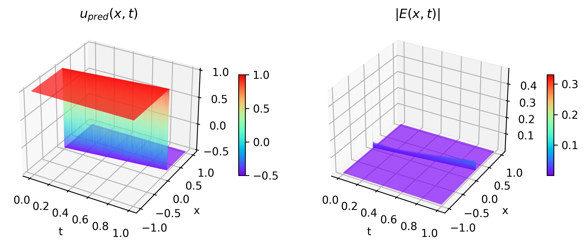
After completing the training process, we investigate the accuracy in the -norm (4.2) and the -norm (4.3) at specific time. The results of the steady shock case are shown in Table 3 and those of the moving shock case appear in Table 4. We observe that for both cases, sl-PINN obtains accurate precision for all the small and . On the contrary, the usual PINN has limited accuracy even for the case when a relatively large is considered. The solution plots of PINN and sl-PINN predictions for the moving shock case when and appear in Figures 4.11 and 4.12, their temporal snapshots in Figures 4.13 and 4.15, and their error plots in Figures 4.14 and 4.16. We find that sl-PINN is capable to capture the stiff behaviour of the Burgers’ solution near the shock for a larger to a smaller .
We note that the initial data in these experiments are discontinuous. It is well-known that neural networks (or any traditional numerical method) have limited performance in fitting a target function with discontinuity [18, 21]. Therefore, as seen in the predictions of the sl-PINN in Figure 4.11 or 4.12, a large error near the singular layer is somewhat expected.


| PINNs | sl-PINNs | |
|---|---|---|
| 6.77E-01 | 4.34E-03 | |
| 1.08E+00 | 4.28E-03 | |
| 6.84E-01 | 2.70E-03 | |
| 9.29E-01 | 3.74E-03 |
| PINNs | sl-PINNs | |||
|---|---|---|---|---|
| 2.00E+00 | 2.00E+00 | 3.82E-04 | 4.80E-02 | |
| 2.00E+00 | 1.99E+00 | 4.64E-04 | 4.79E-02 | |
| 2.00E+00 | 1.99E+00 | 4.12E-04 | 4.80E-02 | |
| 2.00E+00 | 1.90E+00 | 6.11E-04 | 4.80E-02 | |
| PINNs | sl-PINNs | |
|---|---|---|
| 5.84E-01 | 5.46E-03 | |
| 6.23E-01 | 4.19E-03 | |
| 4.24E-01 | 3.01E-03 | |
| 4.04E-01 | 3.84E-03 |
| PINNs | sl-PINNs | |||
|---|---|---|---|---|
| 1.49E+00 | 1.14E+00 | 1.79E-03 | 2.43E-02 | |
| 1.49E+00 | 1.14E+00 | 2.63E-03 | 3.19E-02 | |
| 1.49E+00 | 1.53E+00 | 2.72E-03 | 4.37E-02 | |
| 1.49E+00 | 1.81E+00 | 3.47E-03 | 6.07E-02 | |


5. Conclusion
In this article, we introduce a new learning method known as sl-PINN to address the one-dimensional viscous Burgers problem with low viscosity, causing a singular interior layer. The method incorporates corrector functions that describe the robust behavior of the solution near the interior layer into the structure of PINNs to improve learning performance in that area. This is achieved through interior analysis, treating the problem as two boundary layer sub-problems. The profile of the corrector functions is studied using asymptotic analysis. Both stationary and moving shock cases have been explored. Numerical experiments show that our sl-PINNs accurately predict the solution for every small viscosity, which, in particular, reduces errors near the interior layer compared to the original PINNs. Our proposed method provides a comprehensive understanding of the solution’s behavior near the interior layer, aiding in capturing the robust part of the training solution. This approach offers a distinct perspective from other existing works [24, 25, 19], achieving better accuracy, especially when the shock is more robust.
Acknowledgment
T.-Y. Chang gratefully was supported by the Graduate Students Study Abroad Program grant funded by the National Science and Technology Council(NSTC) in Taiwan. G.-M. Gie was supported by Simons Foundation Collaboration Grant for Mathematicians. Hong was supported by Basic Science Research Program through the National Research Foundation of Korea (NRF) funded by the Ministry of Education (NRF-2021R1A2C1093579) and by the Korea government(MSIT) (RS-2023-00219980). Jung was supported by National Research Foundation of Korea(NRF) grant funded by the Korea government(MSIT) (No. 2023R1A2C1003120).
References
- [1] Basdevant, C., Deville, M., Haldenwang, P., Lacroix, J.M., Ouazzani, J., Peyret, R., Orlandi, P. and Patera, A. Spectral and finite difference solutions of the Burgers equation. Computers and fluids, 14(1), (1986), pp.23-41.
- [2] Buchanan, J. Robert, and Zhoude Shao. A first course in partial differential equations. 2018.
- [3] Junho Choi, Chang-Yeol Jung, and Hoyeon Lee. On boundary layers for the Burgers equations in a bounded domain. Commun. Nonlinear Sci. Numer. Simul., 67:637–657, 2019.
- [4] Choi, Junho and Hong, Youngjoon and Jung, Chang-Yeol and Lee, Hoyeon. Viscosity approximation of the solution to Burgers’ equations with shock layers Appl. Anal., Vol. 102, no. 1, 288–314, 2023.
- [5] Cole, Julian D. On a quasi-linear parabolic equation occurring in aerodynamics. Quarterly of Applied Mathematics. 9 (3): 225–236. (1951).
- [6] Caldwell, J., and P. Smith. Solution of Burgers’ equation with a large Reynolds number. Applied Mathematical Modelling 6, no. 5 (1982): 381-385.
- [7] Debnath, Lokenath. Nonlinear partial differential equations for scientists and engineers. Boston: Birkhäuser, 2005.
- [8] T.-Y. Chang, G.-M. Gie, Y. Hong, and C.-Y. Jung. Singular layer Physics Informed Neural Network method for Plane Parallel Flows Computers and Mathematics with Applications, Volume 166, 2024, 91–105, ISSN 0898–1221
- [9] G.-M. Gie, Y. Hong, C.-Y. Jung, and D. Lee. Semi-analytic physics informed neural network for convection-dominated boundary layer problems in 2D Submitted
- [10] G.-M. Gie, Y. Hong, C.-Y. Jung, and T. Munkhjin. Semi-analytic PINN methods for boundary layer problems in a rectangular domain Journal of Computational and Applied Mathematics, Volume 450, 2024, 115989, ISSN 0377-0427
- [11] G.-M. Gie, Y. Hong, and C.-Y. Jung. Semi-analytic PINN methods for singularly perturbed boundary value problems Applicable Analysis, Published online: 08 Jan 2024
- [12] G.-M. Gie, C.-Y. Jung, and H. Lee. Semi-analytic shooting methods for Burgers’ equation. Journal of Computational and Applied Mathematics, Vol. 418, 2023, 114694, ISSN 0377-0427
- [13] G.-M. Gie, M. Hamouda, C.-Y. Jung, and R. Temam, Singular perturbations and boundary layers, volume 200 of Applied Mathematical Sciences. Springer Nature Switzerland AG, 2018. https://doi.org/10.1007/978-3-030-00638-9
- [14] Hopf, Eberhard. The partial differential equation . Communications on Pure and Applied Mathematics, 3 (3): 201–230. (1950).
- [15] Hon, Yiu-Chung, and X. Z. Mao. An efficient numerical scheme for Burgers’ equation. Applied Mathematics and Computation 95, no. 1 (1998): 37-50.
- [16] Howison, Sam. Practical applied mathematics: modelling, analysis, approximation. No. 38. Cambridge university press, 2005.
- [17] Jagtap, Ameya D., and George Em Karniadakis. Extended physics-informed neural networks (XPINNs): A generalized space-time domain decomposition based deep learning framework for nonlinear partial differential equations. Communications in Computational Physics 28, no. 5 (2020).
- [18] Jagtap, Ameya D., Kenji Kawaguchi, and George Em Karniadakis. Adaptive activation functions accelerate convergence in deep and physics-informed neural networks. Journal of Computational Physics 404 (2020): 109136.
- [19] L. Lu, X. Meng, Z. Mao, G. E. Karniadakis. Deepxde: A deep learning library for solving differential equations. SIAM Review, 63 (1) (2021) 208–228.
- [20] Olver, Peter J. Introduction to partial differential equations. Vol. 1. Berlin: Springer, 2014.
- [21] Nasim Rahaman, Aristide Baratin, Devansh Arpit, Felix Draxler, Min Lin, Fred Hamprecht, Yoshua Bengio, and Aaron Courville. On the Spectral Bias of Neural Networks. Proceedings of the 36th International Conference on Machine Learning, 97 (2019).
- [22] M. Raissi, P. Perdikaris, and G. E. Karniadakis. Physics-informed neural networks: a deep learning framework for solving forward and inverse problems involving nonlinear partial differential equations. J. Comput. Phys., 378 (2019), pp. 686–707.
- [23] S. Shih and R. B. Kellogg, Asymptotic analysis of a singular perturbation problem. SIAM J. Math. Anal. 18 (1987), pp . 1467-1511.
- [24] Song, Y., Wang, H., Yang, H., Taccari, M.L. and Chen, X. Loss-attentional physics-informed neural networks. Journal of Computational Physics, 501, p.112781. , 2024
- [25] Zhuang, Qiao, Chris Ziyi Yao, Zhongqiang Zhang, and George Em Karniadakis. Two-scale Neural Networks for Partial Differential Equations with Small Parameters. arXiv preprint arXiv:2402.17232 (2024).