This paper was converted on www.awesomepapers.org from LaTeX by an anonymous user.
Want to know more? Visit the Converter page.

Single-qubit measurement of two-qubit entanglement in generalized Werner states

Salini Rajeev Department of Physics, 145 Physical Sciences Bldg., Oklahoma State University, Stillwater, OK 74078, USA.    Mayukh Lahiri [email protected] Department of Physics, 145 Physical Sciences Bldg., Oklahoma State University, Stillwater, OK 74078, USA.
Abstract

Conventional methods of measuring entanglement in a two-qubit photonic mixed state require the detection of both qubits. We generalize a recently introduced method which does not require the detection of both qubits, by extending it to cover a wider class of entangled states. Specifically, we present a detailed theory that shows how to measure entanglement in a family of two-qubit mixed states — obtained by generalizing Werner states — without detecting one of the qubits. Our method is interferometric and does not require any coincidence measurement or postselection. We also perform a quantitative analysis of anticipated experimental imperfections to show that the method is experimentally implementable and resistant to experimental losses.

I Introduction

Traditional methods of characterizing entanglement in two-photon mixed states (e.g., the violation of Bell’s inequalities Freedman and Clauser (1972); Aspect et al. (1982); Ou et al. (1992); Giustina et al. (2015), quantum state tomography James et al. (2001), etc.) require detection of both photons (see, for example, Gühne and Tóth (2009); Friis et al. (2019) and references therein). These methods, therefore, involve coincidence measurement or postselection. Methods that do not require detection of both photons rely on the assumption that the quantum state is pure (see, for example, Walborn et al. (2006); Sahoo et al. (2020); Bhattacharjee et al. (2022); Di Lorenzo Pires et al. (2009); Just et al. (2013); Sharapova et al. (2015)).

Recently, it has been demonstrated theoretically Lahiri et al. (2021) and experimentally Lemos et al. (2023) that it is possible to measure entanglement of a special class of two-photon mixed states — obtained by generalizing Bell states — without detecting one of the photons and without employing coincidence measurement or postselection. Density matrices representing such states have two generally non-vanishing coherence terms (off-diagonal elements). The states are entangled if and only if these coherence terms are nonzero. Furthermore, these two coherence terms are complex conjugate of each other. Therefore, entanglement of the states considered in Refs. Lahiri et al. (2021); Lemos et al. (2023) is fully characterized by one coherence term of the corresponding density matrix. However, entanglement of most two-qubit states are not dependent on their density matrix elements in such a trivial manner, e.g., the Werner state that can be entangled without violating Bell’s inequalities Werner (1989). Whether the entanglement of any two-qubit photonic mixed state can be verified by detecting one qubit remains an open question of fundamental importance.

Here, we take an important step toward answering this question by extending the method to two-qubit mixed states that can be obtained by generalizing Werner states. We find that albeit the same principle introduced in Refs. Lahiri et al. (2021); Lemos et al. (2023) applies, the measurement procedure requires considerable modifications. Our results also suggest that the method to account for experimental losses would require significant adaptation (Supplementary Material).

The article is organized as follows: In Sec. II, we discuss the class of quantum state we address and their entanglement. In Sec. III, we provide an outline of the entanglement measurement scheme. In Sec. IV we present a detailed theoretical analysis and our main results. We also illustrate the results by numerical examples. In Sec. V we compare our results with existing ones. In Sec. VI, we discuss the effect of anticipated experimental imperfections. Finally, we summarize and conclude in Sec. VII.

II Two-Qubit Generalized Werner State and Its Entanglement

Refer to caption
Figure 1: Illustration of the PPT criterion applied to generalized Werner states. The state is entangled when the eigenvalue α1<0\alpha_{1}<0 (shaded regions). The black filled circle and the red diamond represent a Bell state (|Φ+|\Phi^{+}\rangle or |Φ|\Phi^{-}\rangle) and a Werner state, respectively. a, α1\alpha_{1} is plotted against η\eta for =1\mathscr{I}=1 and IH=0.5I_{H}=0.5 (solid line), for =0.8\mathscr{I}=0.8 and IH=0.3I_{H}=0.3 (dashed line), and for =0.3\mathscr{I}=0.3 and IH=0.8I_{H}=0.8 (dash-dotted line). b, α1\alpha_{1} is plotted against IHI_{H} for =1\mathscr{I}=1 and η=1\eta=1 (solid line), for =0.8\mathscr{I}=0.8 and η=0.8\eta=0.8 (dashed line), and for =1\mathscr{I}=1 and η=0.45\eta=0.45 (dash-dotted line). c, α1\alpha_{1} is plotted against \mathscr{I} for IH=0.5I_{H}=0.5 and η=1\eta=1 (solid line), IH=0.5I_{H}=0.5 and η=0.8\eta=0.8 (dashed line), and IH=0.6I_{H}=0.6 and η=0.5\eta=0.5 (dash-dotted line).

We work with a two-photon polarization state that is a common test bed for two-qubit systems. Throughout this paper, we call the two photons forming a pair signal (SS) and idler (II). We use H,V,D,A,RH,V,D,A,R, and LL to represent horizontal, vertical, diagonal, antidiagonal, right-circular, and left-circular polarization, respectively. The ket, |μI,νS|\mu_{I},\nu_{S}\rangle, represents a photon pair where the idler photon has polarization μ\mu and the signal photon has polarization ν\nu.

The quantum state considered here is obtained by generalizing the Werner state. The density matrix takes the following form in the computational basis {|HIHS,|HIVS,|VIHS,|VIVS}\{|H_{I}H_{S}\rangle,|H_{I}V_{S}\rangle,|V_{I}H_{S}\rangle,|V_{I}V_{S}\rangle\}:

ρ^=(ηIH+1η400ηIHIVeiϕ01η400001η40ηIHIVeiϕ00ηIV+1η4),\displaystyle\widehat{\rho}=\begin{pmatrix}\eta I_{H}+\frac{1-\eta}{4}&0&0&\eta\mathscr{I}\sqrt{I_{H}I_{V}}e^{-i\phi}\\ 0&\frac{1-\eta}{4}&0&0\\ 0&0&\frac{1-\eta}{4}&0\\ \eta\mathscr{I}\sqrt{I_{H}I_{V}}e^{i\phi}&0&0&\eta I_{V}+\frac{1-\eta}{4}\end{pmatrix}, (1)

where 0IH10\leq I_{H}\leq 1, IV=1IHI_{V}=1-I_{H}, 0η10\leq\eta\leq 1, 010\leq\mathscr{I}\leq 1, and ϕ\phi represents a phase. It can be immediately checked that this state becomes a Werner state when IH=IV=1/2I_{H}=I_{V}=1/2 and =1\mathscr{I}=1. For IH=IV=1/2I_{H}=I_{V}=1/2, =1\mathscr{I}=1 and η=1\eta=1, it reduces to Bell states |Φ+=(|HIHS+|VIVS)/2|\Phi^{+}\rangle=(|H_{I}H_{S}\rangle+|V_{I}V_{S}\rangle)/\sqrt{2} and |Φ=(|HIHS|VIVS)/2|\Phi^{-}\rangle=(|H_{I}H_{S}\rangle-|V_{I}V_{S}\rangle)/\sqrt{2} when ϕ=0\phi=0 and ϕ=π\phi=\pi, respectively. Therefore, the state given by Eq. (1) can also be obtained by the convex combination of a fully mixed state with the generalization of Bell states considered in Refs. Lahiri et al. (2021); Lemos et al. (2023).

The entanglement of this state can be verified by testing the positive partial transpose (PPT) criterion Peres (1996). A partial transposition of the density matrix (ρ^\widehat{\rho}) is a transposition taken with respect to only one of the photons. The density matrix has a positive partial transpose if and only if its partial transposition does not have any negative eigenvalues. Since we have a 2×22\times 2 system, according to the PPT criterion the state is entangled if and only if it does not have a positive partial transpose Horodecki (1997).

By determining the eigenvalues of a partial transpose of the density matrix given by Eq. (1), we find that three of them are always positive (see Appendix A). The only eigenvalue that can be negative is given by

α1=1η4ηIHIV4.\alpha_{1}=\frac{1-\eta-4\eta\mathscr{I}\sqrt{I_{H}I_{V}}}{4}. (2)

Figure 1 illustrates entanglement of generalized Werner states (ρ^\widehat{\rho}) characterized by the PPT criterion for various choices of state parameters η\eta, IHI_{H}, and \mathscr{I}.

The amount of entanglement present in the quantum state can be quantified by the concurrence Wootters (1998). We find that the concurrence of the state given by Eq. (1) is (see Appendix B)

C(ρ^)=max{η1+4ηIHIV2,0}.\displaystyle C(\widehat{\rho})=\text{max}\left\{\frac{\eta-1+4\eta\mathscr{I}\sqrt{I_{H}I_{V}}}{2},0\right\}. (3)

We show below how to determine the concurrence without detecting one of the photons.

III Outline of the Entanglement Measurement Scheme

The principle of our method is based on a unique quantum interference phenomenon that was first demonstrated by Zou, Wang, and Mandel Zou et al. (1991); Wang et al. (1991) and is sometimes called the interference by path identity Hochrainer et al. (2022). The method employs a nonlinear interferometer Chekhova and Ou (2016) that contains two identical twin-photon sources. Each source produces the same quantum state [Eq. (1)].

A conceptual arrangement of the entanglement measurement scheme is illustrated in Fig. 2. The two photon-pair sources are denoted by Q1Q_{1} and Q2Q_{2}. A photon pair is in superposition of being created at the two sources — for sources made of nonlinear crystals, such a situation can be achieved by weakly pumping them with mutually coherent laser beams. The sources do not produce the states simultaneously, i.e., the probability of having more than one photon pair in the system between an emission and a detection is negligible. That is, in this situation the effect of stimulated (induced) emission is negligible Zou et al. (1991); Wang et al. (1991); Wiseman and Mølmer (2000); Liu et al. (2009); Lahiri et al. (2019).

Refer to caption
Figure 2: Entanglement measurement scheme. Two sources (Q1Q_{1} and Q2Q_{2}) can individually generate the two-qubit photonic state ρ^\widehat{\rho} [Eq. (1)]. Q1Q_{1} emits a photon pair, signal and idler, into propagation modes S1S_{1} and I1I_{1}. Likewise, Q2Q_{2} emits signal and idler photons into modes S2S_{2} and I2I_{2}. Modes S1S_{1} and S2S_{2} are combined by a beamsplitter (BSBS) and the signal photon emerging from BSBS is sent to a detector after projecting it onto a chosen polarization state (μ=H\mu=H, VV, DD, AA, RR, or LL). Modes I1I_{1} and I2I_{2} are made identical by aligning the corresponding beams without the use of a beamsplitter. This alignment makes it impossible to know from which source a signal photon originated and consequently, a single-photon interference pattern appears at the detector. The idler photon is never detected and no postselection is considered to obtain the interference pattern. A unitary transformation, U(θ,δ)U(\theta,\delta), is performed on the idler photon between the two sources. The information about the entanglement is extracted from the interference patterns with the knowledge of this transformation.

Signal beams (S1S_{1} and S2S_{2}) from the two sources are superposed by a balanced beamsplitter and the single-photon counting rate (intensity) is measured at one of the outputs of the beamsplitter. The idler beam from Q1Q_{1} is sent through Q2Q_{2} and is aligned with the idler beam generated by Q2Q_{2}. (Such an alignment was originally suggested by Z. Y. Ou Zou et al. (1991).) This alignment makes it impossible to know from which source the signal photon originated. Consequently, a single-photon interference pattern appears at a detector placed at an output of the beamsplitter. Details of experimental conditions to obtain the interference pattern have been discussed in numerous publications (see, for example, Wang et al. (1991); Lemos et al. (2022a, b)).

We apply a unitary transformation on the field representing the idler photon between the two sources. Such transformations can readily be implemented in a laboratory using quarter- and half-wave plates. We choose a unitary transformation that is characterized by two controllable parameters (δ\delta and θ\theta) and has the following form in the {|H,|V}\{|H\rangle,|V\rangle\} basis:

U(θ,δ)=(eiδcos2θeiδsin2θeiδsin2θeiδcos2θ),\displaystyle U(\theta,\delta)=\begin{pmatrix}e^{-i\delta}\cos 2\theta&e^{-i\delta}\sin 2\theta\\ e^{i\delta}\sin 2\theta&-e^{i\delta}\cos 2\theta\end{pmatrix}, (4)

where 0θπ0\leq\theta\leq\pi and 0δ/2π0\leq\delta/2\leq\pi can be understood as two half-wave plate angles.

The fact that we can fully control the choice of θ\theta and δ\delta plays crucial role in our measurement scheme. We show below that the effect of this unitary transformation appears in the interference patterns generated by the signal photon after it is projected onto appropriate polarization states. We also show how the entanglement of ρ^\widehat{\rho} can be fully characterized from these single-photon interference patterns with the knowledge of the unitary transformation. For simplicity, we initially assume that there is no experimental loss. In the supplementary material, we provide a detailed description of how to treat dominant experimental losses and imperfections. We discuss the effects of experimental imperfections in Sec. VI.

We emphasize that the signal photon never interacts with the device performing the unitary transformation and the idler photon is never detected. These are two unique features of our entanglement measurement scheme in addition to the fact that no postselection or coincidence measurement is required.

IV Theoretical Analysis

IV.1 Determining the quantum state

We use the standard bra-ket notation for the convenience of analysis. The generalized Werner state [Eq. (1)] in the bra-ket notation takes the form

ρ^=μ,νH,Vμ,νH,VμIνS|ρ^|μIνS|μIνSμIνS|,\displaystyle\widehat{\rho}=\sum_{\mu,\nu}^{H,V}\sum_{\mu^{\prime},\nu^{\prime}}^{H,V}\langle\mu_{I}\nu_{S}|\widehat{\rho}|\mu_{I}^{\prime}\nu_{S}^{\prime}\rangle|\mu_{I}\nu_{S}\rangle\langle\mu_{I}^{\prime}\nu_{S}^{\prime}|, (5)

where μIνS|ρ^|μIνS\langle\mu_{I}\nu_{S}|\widehat{\rho}|\mu_{I}^{\prime}\nu_{S}^{\prime}\rangle represents a matrix element; for example, HIHS|ρ^|HIHS=ηIH+(1η)/4\langle H_{I}H_{S}|\widehat{\rho}|H_{I}H_{S}\rangle=\eta I_{H}+(1-\eta)/4.

Equation (5) [or equivalently, Eq. (1)] is the state generated by an individual source. While determining the quantum state generated by the two sources jointly, one needs to use the fact that the probability of emission of more than one photon pair is negligible, that is, the total occupation number of photons in the state is always two.

We first consider the scenario in which the idler beams are not aligned. In this case, a signal photon is in a superposition of being in modes S1S_{1} and S2S_{2} that emerges from two sources. Likewise, an idler photon is in a superposition of being in modes I1I_{1} and I2I_{2}. Consequently, the density matrix representing the quantum state produced jointly by the two sources becomes an 8×88\times 8 matrix. We determine this matrix following the approach introduced in Ref. Lahiri et al. (2021) and represent it by bra-ket notation [Appendix C, Eq. (Appendix C: The two-photon density matrix)].

We now analytically represent the alignment of idler beams. Modes I1I_{1} and I2I_{2} becomes identical due to this alignment. The alignment, together with the unitary transformation [Eq. (4)] applied on the idler photon, results in the following transformations of kets:

|HI2=eiϕI(eiδcos2θ|HI1+eiδsin2θ|VI1),\displaystyle|H_{I_{2}}\rangle=e^{-i\phi_{I}}\left(e^{i\delta}\cos 2\theta|H_{I_{1}}\rangle+e^{i\delta}\sin 2\theta|V_{I_{1}}\rangle\right), (6a)
|VI2=eiϕI(eiδsin2θ|HI1eiδcos2θ|VI1),\displaystyle|V_{I_{2}}\rangle=e^{-i\phi_{I}}\left(e^{-i\delta}\sin 2\theta|H_{I_{1}}\rangle-e^{-i\delta}\cos 2\theta|V_{I_{1}}\rangle\right), (6b)

where ϕI\phi_{I} is the phase acquired by propagation from Q1Q_{1} to Q2Q_{2}.

Finally, we obtain the density matrix, ρ^(f)\widehat{\rho}^{(f)}, representing the photon pair in our system (before arriving at BSBS) by substituting from Eqs. (6a) and (6b) into the 8×88\times 8 density matrix [Appendix C, Eq. (Appendix C: The two-photon density matrix)] mentioned above. An expression for ρ^(f)\widehat{\rho}^{(f)} is given by Eq. (Appendix C: The two-photon density matrix) in Appendix C. The probability of detecting a signal photon at one of the outputs of BSBS (Fig. 2) can be determined using this density matrix or from the reduced density matrix (ρ^S\widehat{\rho}_{S}) obtained by taking partial trace of ρ^(f)\widehat{\rho}^{(f)} over the subspace of the idler photon. Here, we take the later approach. The reduced density matrix representing a signal photon before arriving at BSBS is given by

ρ^S\displaystyle\widehat{\rho}_{S} =K(η,IH)(|b1|2|HS1HS1|+|b2|2|HS2HS2|)+K(η,IV)(|b1|2|VS1VS1|+|b2|2|VS2VS2|)\displaystyle=K(\eta,I_{H})\left(|b_{1}|^{2}|H_{S_{1}}\rangle\langle H_{S_{1}}|+|b_{2}|^{2}|H_{S_{2}}\rangle\langle H_{S_{2}}|\right)+K(\eta,I_{V})\left(|b_{1}|^{2}|V_{S_{1}}\rangle\langle V_{S_{1}}|+|b_{2}|^{2}|V_{S_{2}}\rangle\langle V_{S_{2}}|\right)
+{b1b2eiϕI[{(η,IH,δ)|HS1HS2|+(η,IV,δ)|VS1VS2|}cos2θ\displaystyle+\Big{\{}b_{1}b_{2}^{\ast}e^{i\phi_{I}}\big{[}\left\{\mathscr{L}(\eta,I_{H},\delta)|H_{S_{1}}\rangle\langle H_{S_{2}}|+\mathscr{L}^{\prime}(\eta,I_{V},\delta)|V_{S_{1}}\rangle\langle V_{S_{2}}|\right\}\cos 2\theta
+ηIHIV{Φ(δ)|HS1VS2|+Φ(δ)|VS1HS2|}sin2θ]+H.c.},\displaystyle\qquad\qquad\quad+\eta\mathscr{I}\sqrt{I_{H}I_{V}}\left\{\Phi(\delta)|H_{S_{1}}\rangle\langle V_{S_{2}}|+\Phi^{\prime}(\delta)|V_{S_{1}}\rangle\langle H_{S_{2}}|\right\}\sin 2\theta\big{]}+\text{H.c.}\Big{\}}, (7)

where |bj|2|b_{j}|^{2} is the probability of emission from source QjQ_{j}, H.c. represents the Hermitian conjugation, K(η,I)=ηI+(1η)/2K(\eta,I)=\eta I+(1-\eta)/2, Φ(δ)=exp[i(ϕH1,H1V2,V2+δ)]\Phi(\delta)=\exp[i(\phi^{V_{2},V_{2}}_{H_{1},H_{1}}+\delta)], Φ(δ)=exp[i(ϕV1,V1H2,H2δ)]\Phi^{\prime}(\delta)=\exp[i(\phi^{H_{2},H_{2}}_{V_{1},V_{1}}-\delta)], and

(η,IH,δ)=\displaystyle\mathscr{L}(\eta,I_{H},\delta)= M(η,IH)exp[i(ϕH1,H1H2,H2δ)]\displaystyle M(\eta,I_{H})\exp\left[i\left(\phi^{H_{2},H_{2}}_{H_{1},H_{1}}-\delta\right)\right]
N(η)exp[i(ϕV1,H1V2,H2+δ)],\displaystyle-N(\eta)\exp\left[i\left(\phi^{V_{2},H_{2}}_{V_{1},H_{1}}+\delta\right)\right], (8a)
(η,IV,δ)=\displaystyle\mathscr{L}^{\prime}(\eta,I_{V},\delta)= N(η)exp[i(ϕH1,V1H2,V2δ)]\displaystyle N(\eta)\exp\left[i\left(\phi^{H_{2},V_{2}}_{H_{1},V_{1}}-\delta\right)\right]
M(η,IV)exp[i(ϕV1,V1V2,V2+δ)],\displaystyle-M(\eta,I_{V})\exp\left[i\left(\phi^{V_{2},V_{2}}_{V_{1},V_{1}}+\delta\right)\right], (8b)

with M(η,I)=(4ηI+1η)/4M(\eta,I)=(4\eta I+1-\eta)/4 and N(η)=(1η)/4N(\eta)=(1-\eta)/4. We observe that all state parameters (η\eta, IHI_{H}, and \mathscr{I}) and the unitary transformation parameters (θ\theta and δ\delta) appear in the density matrix representing a signal photon.

IV.2 Information of entanglement in Interference Patterns

As mentioned in Sec. III, signal beams S1S_{1} and S2S_{2} are superposed by a balanced beamsplitter (BS), one of the outputs of BS is projected onto a particular polarization state, and then sent to a detector. Therefore, the positive-frequency part of the quantized electric field at the detector is given by

E^μS(+)=12(a^μS1+ieiϕSa^μS2),\displaystyle\widehat{E}^{(+)}_{\mu_{S}}=\frac{1}{\sqrt{2}}\big{(}\widehat{a}_{\mu_{S1}}+ie^{i\phi_{S}}\widehat{a}_{\mu_{S2}}\big{)}, (9)

where μ=H,V,D,A,R,L\mu=H,V,D,A,R,L and a^μSj\widehat{a}_{\mu_{Sj}} is the annihilation operator corresponding to signal photon with polarization μ\mu emitted by source QjQ_{j}. The probability of detecting a signal photon with polarization μ\mu is obtained by the standard formula Glauber (1963)

Pμ=tr{ρ^SE^μS()E^μS(+)},\displaystyle P_{\mu}=\text{tr}\left\{\widehat{\rho}_{S}\widehat{E}^{(-)}_{\mu_{S}}\widehat{E}^{(+)}_{\mu_{S}}\right\}, (10)

where E^μS()={E^μS(+)}\widehat{E}^{(-)}_{\mu_{S}}=\{\widehat{E}^{(+)}_{\mu_{S}}\}^{{\dagger}} and ρ^S\widehat{\rho}_{S} is given by Eq. (IV.1). The single-photon counting rate (intensity) at the detector is linearly proportional to the probability PμP_{\mu}. We show below that these photon counting rates represent interference patterns. The state parameters (η,IH,\eta,I_{H},\mathscr{I}) that characterize the entanglement appear in the expressions for these interference patterns.

We first determine the photon counting rate at the detector when the signal photon is projected onto the horizontally polarized (H) state. It follows from Eqs. (IV.1) – (10) that (Appendix D)

PH|θ=0\displaystyle P_{H}\big{|}_{\theta=0} =12[P1+P2+2|b1||b2|sin(ϕin+ϕ0)\displaystyle=\frac{1}{2}\big{[}P_{1}+P_{2}+2|b_{1}||b_{2}|\sin\left(\phi_{\text{in}}+\phi_{0}\right)
×{P12+P222P1P2cos(χ+2δ)}12],\displaystyle\times\{P_{1}^{2}+P_{2}^{2}-2P_{1}P_{2}\cos(\chi+2\delta)\}^{\frac{1}{2}}\big{]}, (11)

where ϕin\phi_{\text{in}}=arg{b1}arg{b2}+ϕIϕS\arg\{b_{1}\}-\arg\{b_{2}\}+\phi_{I}-\phi_{S}, P1=ηIH+(1η)/4P_{1}=\eta I_{H}+(1-\eta)/4, P2=(1η)/4P_{2}=(1-\eta)/4, χ=ϕV1H1V2H2ϕH1H1H2H2\chi=\phi^{V_{2}H_{2}}_{V_{1}H_{1}}-\phi^{H_{2}H_{2}}_{H_{1}H_{1}} and ϕ0=ϕH1H1H2H2δ+ϵ1\phi_{0}=\phi_{H_{1}H_{1}}^{H_{2}H_{2}}-\delta+\epsilon_{1}; the explicit form of ϵ1\epsilon_{1} is not required for our purpose. It is evident from Eq. (IV.2) that the value of PH|θ=0P_{H}\big{|}_{\theta=0} changes sinusoidally as ϕin\phi_{\text{in}} is varied, i.e., Eq. (IV.2) represents an interference pattern. Here, we have chosen θ=0\theta=0 to maximize the contribution from the interference term (general expressions are given in Appendix D).

Equation (IV.2) shows that the visibility depends on the parameter δ\delta that one can fully control in an experiment. We set δ=δH\delta=\delta_{H} such that the visibility attains its minimum non-zero value, i.e, cos(χ+2δH)=1\cos(\chi+2\delta_{H})=1. The expression for PHP_{H} then becomes

PH|θ=0δ=δH=1η4+ηIH2+|b1||b2|ηIHsin(ϕin+ϕ0),\displaystyle P_{H}\big{|}_{\theta=0}^{\delta=\delta_{H}}=\frac{1-\eta}{4}+\frac{\eta I_{H}}{2}+|b_{1}||b_{2}|\eta I_{H}\sin(\phi_{\text{in}}+\phi_{0}), (12)

and consequently, the visibility is given by 111The visibility is determined by the standard formula 𝒱μ=(PμmaxPμmin)/(Pμmax+Pμmin)\mathcal{V}_{\mu}=\left(P^{\text{max}}_{\mu}-P^{\text{min}}_{\mu}\right)/\left(P^{\text{max}}_{\mu}+P^{\text{min}}_{\mu}\right).

𝒱H|θ=0δ=δH=4|b1||b2|ηIH2ηIH+1η.\displaystyle\mathcal{V}_{H}\big{|}_{\theta=0}^{\delta=\delta_{H}}=\frac{4|b_{1}||b_{2}|\eta I_{H}}{2\eta I_{H}+1-\eta}. (13)

Likewise, we find that the visibility of the single-photon interference pattern for VV polarization is

𝒱V|θ=0δ=δV=4|b1||b2|η(1IH)1+η2ηIH,\displaystyle\mathcal{V}_{V}\big{|}_{\theta=0}^{\delta=\delta_{V}}=\frac{4|b_{1}||b_{2}|\eta(1-I_{H})}{1+\eta-2\eta I_{H}}, (14)

where δV\delta_{V} plays the same role as δH\delta_{H} in Eq. (13).

State (η,,IH\eta,\mathscr{I},I_{H}) 𝒱R|θ=π4\mathcal{V}_{R}|_{\theta=\frac{\pi}{4}} 𝒱D|θ=π4\mathcal{V}_{D}|_{\theta=\frac{\pi}{4}} 𝒱V|θ=0δ=δV\mathcal{V}_{V}\big{|}_{\theta=0}^{\delta=\delta_{V}} 𝒱H|θ=0δ=δH\mathcal{V}_{H}\big{|}_{\theta=0}^{\delta=\delta_{H}} PPT Criterion Concurrence
ρ^1\widehat{\rho}_{1} (0.0, –, –) 0.00 0.00 0.00 0.00 Separable 0.00
ρ^2\widehat{\rho}_{2} (0.2, 1.0, 0.5) 0.08 0.18 0.20 0.20 Separable 0.00
ρ^3\widehat{\rho}_{3} (0.6, 0.8, 0.3) 0.17 0.41 0.67 0.47 Entangled 0.24
ρ^4\widehat{\rho}_{4} (0.7, 1.0, 0.5) 0.27 0.64 0.70 0.70 Entangled 0.55
ρ^5\widehat{\rho}_{5} (1.0, 1.0, 0.5) 0.38 0.92 1.00 1.00 Entangled 1.00
Table 1: Numerical results illustrating entanglement verification for five quantum states through single-photon interference.

We now consider the remaining cases where the signal photon is projected onto diagonal (D), antidiagonal (A), right-circular (R), and left-circular (L) polarizations. General expressions for single-photon counting rates for all these cases are given in Appendix D. Using those expressions [Eqs. (D5a)–(D5d)], we obtain the corresponding formulas for visibility as

𝒱D|θ=π4=𝒱A|θ=π4\displaystyle\mathcal{V}_{D}\big{|}_{\theta=\frac{\pi}{4}}=\mathcal{V}_{A}\big{|}_{\theta=\frac{\pi}{4}}
=2|b1||b2|ηIHIV2+2cos(χ2δ),\displaystyle=2|b_{1}||b_{2}|\eta\mathscr{I}\sqrt{I_{H}I_{V}}\sqrt{2+2\cos(\chi^{\prime}-2\delta)}, (15)

and

𝒱R|θ=π4=𝒱L|θ=π4\displaystyle\mathcal{V}_{R}\big{|}_{\theta=\frac{\pi}{4}}=\mathcal{V}_{L}\big{|}_{\theta=\frac{\pi}{4}}
=2|b1||b2|ηIHIV22cos(χ2δ),\displaystyle=2|b_{1}||b_{2}|\eta\mathscr{I}\sqrt{I_{H}I_{V}}\sqrt{2-2\cos(\chi^{\prime}-2\delta)}, (16)

where χ\chi^{\prime} is given in Appendix D (its explicit form is not required for our purpose).

Equations (13)–(16) show that all parameters that characterize the entanglement appear in the expressions for visibility for HH, VV, DD, AA, RR, and LL polarizations. That is, the information about the entanglement is contained in the single-photon interference patterns obtained by detecting one of the qubits only.

IV.3 Entanglement Verification and Measurement

We now show how to test the PPT criterion and to measure the concurrence from the single-photo interference patterns. It follows from Eqs. (2) and (3) that it is enough to represent η\eta and ηIHIV\eta\mathscr{I}\sqrt{I_{H}I_{V}} in terms of experimentally measurable quantities. We show below that these two quantities can be directly obtained from the expressions for visibilities given in Sec. IV.2. That is, we do not need to determine all state parameters (η\eta, IHI_{H}, and \mathscr{I}) individually.

We first express |b1||b2||b_{1}||b_{2}| in terms of experimentally measurable quantities. We recall that |b1|2|b_{1}|^{2} and |b2|2|b_{2}|^{2} are probabilities of emission from sources Q1Q_{1} and Q2Q_{2}, respectively. Suppose that Pμ(1)P_{\mu}^{(1)} is the probability of detecting a signal photon with polarization μ\mu (μ=H,V\mu=H,V) when signal beam, S2S_{2}, emerging from Q2Q_{2} is blocked. Likewise, Pμ(2)P_{\mu}^{(2)} is the detection-probability when signal beam S1S_{1} is blocked. We thus have

|b1||b2|=Pμ(1)Pμ(2)Pμ(1)+Pμ(2).\displaystyle|b_{1}||b_{2}|=\frac{\sqrt{P_{\mu}^{(1)}P_{\mu}^{(2)}}}{P_{\mu}^{(1)}+P_{\mu}^{(2)}}. (17)

We now apply Eqs. (13) and (14) to determine η\eta and find that

η=𝒱V|θ=0δ=δV+𝒱H|θ=0δ=δH1|b1||b2|𝒱H|θ=0δ=δH𝒱V|θ=0δ=δV4|b1||b2|𝒱V|θ=0δ=δV𝒱H|θ=0δ=δH.\displaystyle\eta=\frac{\mathcal{V}_{V}\big{|}_{\theta=0}^{\delta=\delta_{V}}+\mathcal{V}_{H}\big{|}_{\theta=0}^{\delta=\delta_{H}}-\frac{1}{|b_{1}||b_{2}|}\mathcal{V}_{H}\big{|}_{\theta=0}^{\delta=\delta_{H}}\mathcal{V}_{V}\big{|}_{\theta=0}^{\delta=\delta_{V}}}{4|b_{1}||b_{2}|-\mathcal{V}_{V}\big{|}_{\theta=0}^{\delta=\delta_{V}}-\mathcal{V}_{H}\big{|}_{\theta=0}^{\delta=\delta_{H}}}. (18)

It can be checked that when |b1|=|b2|=1/2|b_{1}|=|b_{2}|=1/\sqrt{2}, the right-hand side of Eq. (18) becomes equal to 1 in the limit 𝒱H|θ=0δ=δH1\mathcal{V}_{H}\big{|}_{\theta=0}^{\delta=\delta_{H}}\to 1- and 𝒱V|θ=0δ=δV1\mathcal{V}_{V}\big{|}_{\theta=0}^{\delta=\delta_{V}}\to 1-. In this limit, the generalized Werner state [Eq. (1)] reduces to the generalization of Bell states considered in Refs. Lahiri et al. (2021); Lemos et al. (2023), for which η=1\eta=1. Using Eqs. (17) and (18) one can immediately express η\eta in terms of experimentally measurable quantities.

To determine the quantity ηIHIV\eta\mathscr{I}\sqrt{I_{H}I_{V}}, we eliminate the cosine terms from Eqs. (15) and (16) by squaring and adding them. It then immediately follows that

ηIHIV=14|b1||b2|(𝒱D|θ=π4)2+(𝒱R|θ=π4)2.\displaystyle\eta\mathscr{I}\sqrt{I_{H}I_{V}}=\frac{1}{4|b_{1}||b_{2}|}\sqrt{(\mathcal{V}_{D}|_{\theta=\frac{\pi}{4}})^{2}+(\mathcal{V}_{R}|_{\theta=\frac{\pi}{4}})^{2}}. (19)

Using Eqs. (17) and (19), we can readily express ηIHIV\eta\mathscr{I}\sqrt{I_{H}I_{V}} in terms of photon counting rates and visibilities of single-photon interference patterns.

To test the PPT criterion, we express the eigenvalue, α1\alpha_{1} [Eq. (2)], in terms of experimentally measurable quantities. Using Eq. (2) and Eqs. (17)–(19), we find that

α1=1𝒱HV4𝒱DR4,\displaystyle\alpha_{1}=\frac{1-\mathcal{V}_{HV}-4\mathcal{V}_{DR}}{4}, (20)

where we have denoted the right-hand sides of Eqs. (18) and (19) by 𝒱HV\mathcal{V}_{HV} and 𝒱DR\mathcal{V}_{DR}, respectively. According to the PPT criterion, the state ρ^\widehat{\rho} [Eq. (1)] is entangled if and only if α1<0\alpha_{1}<0, that is, the state is entangled if and only if

𝒱HV+4𝒱DR>1.\displaystyle\mathcal{V}_{HV}+4\mathcal{V}_{DR}>1. (21)

We illustrate the PPT criterion by choosing five quantum states (ρ^1,,ρ^5\widehat{\rho}_{1},\dots,\widehat{\rho}_{5}) in Table 1. The criterion is tested using Eq. (21). For simplicity, we assume that |b1|=|b2|=1/2|b_{1}|=|b_{2}|=1/\sqrt{2}. To compute visibilities for DD and RR polarization, we chose χ2δ=π/4\chi^{\prime}-2\delta=\pi/4. It is to be noted that the entanglement does not depend on the value of χ2δ\chi^{\prime}-2\delta [see Eqs. (15)–(19)].

The state ρ^1\widehat{\rho}_{1} is chosen to be fully mixed. (Note that in this case η=0\eta=0 and values of \mathscr{I} and IHI_{H} are irrelevant.) Applying Eq. (21), we find that ρ^1\widehat{\rho}_{1} is separable as one would expect. The state ρ^2\widehat{\rho}_{2} is chosen as a Werner state with η=0.2<1/3\eta=0.2<1/3 and this state is found to be separable as expected. We choose ρ^3\widehat{\rho}_{3} as an entangled mixed state and we find that Eq. (21) verifies that it is entangled. The density matrix ρ^4\widehat{\rho}_{4} represents a Werner state for which η=0.7>1/3\eta=0.7>1/3. We find this state to be entangled. Finally, the state ρ^5\widehat{\rho}_{5} is chosen to be the Bell state, |Φ+=(|HIHS+|VIVS)/2|\Phi^{+}\rangle=(|H_{I}H_{S}\rangle+|V_{I}V_{S}\rangle)/\sqrt{2}. As expected, the state is entangled according to Eq. (21).

In order to express the concurrence in terms of experimentally measurable quantities, we substitute from Eqs. (19) and (18) into Eq. (3) and find that

C(ρ^)=max{0,𝒱HV+4𝒱DR12},\displaystyle C(\widehat{\rho})=\text{max}\Big{\{}0,\frac{\mathcal{V}_{HV}+4\mathcal{V}_{DR}-1}{2}\Big{\}}, (22)

where 𝒱HV\mathcal{V}_{HV} and 𝒱DR\mathcal{V}_{DR} represent right-hand sides of Eqs. (18) and (19), respectively. Equation (22) shows that the concurrence of the two-qubit mixed state can be determined from visibilities of the interference patterns obtained by detecting only one of the qubits.

Refer to caption
Figure 3: Concurrence of five generalized Werner states (Table 1) determined using single-photon visibilities. Simulated data points (filled circles) represent the concurrence computed using state-parameters [Eq. (3)] and the formula max{0,(𝒱HV+4𝒱DR1)/2}\text{max}\{0,(\mathcal{V}_{HV}+4\mathcal{V}_{DR}-1)/2\}. (Data points for ρ^1\widehat{\rho}_{1} and ρ^2\widehat{\rho}_{2} coincide.) All simulated data points lie on the straight line predicted by Eq. (22) showing that the concurrence can be determined from single-photon visibilities.

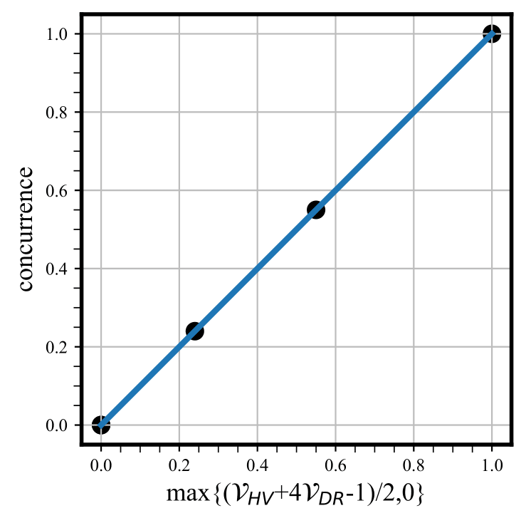
To illustrate Eq. (22), we consider the five quantum states (ρ^1,,ρ^5\widehat{\rho}_{1},\dots,\widehat{\rho}_{5}) given in Table 1 and choose |b1|=|b2|=1/2|b_{1}|=|b_{2}|=1/\sqrt{2} for simplicity. We determine the concurrence of these states using two methods: (i) using the state-parameters [i.e., using Eq. (3); the corresponding values of the concurrence are given in Table 1], and (ii) using the values of visibilities [i.e, the formula max{0,(𝒱HV+2𝒱DR1)/2}\text{max}\{0,(\mathcal{V}_{HV}+2\mathcal{V}_{DR}-1)/2\}]. In Fig. 3 we plot the values of concurrence obtained by method (i) against the values obtained by method (ii), and find that they lie on the straight line predicted by Eq. (22).

We have thus shown that it is possible to test the PPT criterion and measure concurrence for a two-qubit generalized Werner state without detecting one of the qubits.

We have expressed the PPT criterion and the concurrence in terms of interference visibilities to be consistent with existing results Lahiri et al. (2021). We note that they can be equivalently expressed in terms of detection probabilities [see Appendix E, Eqs. (E5) and (E6)]. The latter approach results in simpler theoretical treatment of the problem in the presence of experimental losses (Supplementary Material).

We stress that all state parameters (η\eta, IHI_{H}, and \mathscr{I}) are not required to be determined for verifying and measuring entanglement, albeit they can be determined from the single-photon interference patterns. Equation (18) [or, equivalently, Eq. (E2) of Appendix E] provides an expression for η\eta. Expressions for IHI_{H} and \mathscr{I} are given by Eqs. (F1) and (F2) in Appendix F.

V Comparison with Existing Results

In order to put our work into context with existing work, we now compare our results to those presented in Refs. Lahiri et al. (2021); Lemos et al. (2023). The entanglement of quantum states considered in Refs. Lahiri et al. (2021); Lemos et al. (2023) is fully characterized by one coherence term (off-diagonal element) of the density matrix. Consequently, such states are entangled if 𝒱D|θ=π40\mathcal{V}_{D}|_{\theta=\frac{\pi}{4}}\neq 0 or 𝒱R|θ=π40\mathcal{V}_{R}|_{\theta=\frac{\pi}{4}}\neq 0 and vice versa Lahiri et al. (2021); Lemos et al. (2023). This is no longer the case for generalized Werner states as illustrated by state ρ^2\widehat{\rho}_{2} in Table 1. State ρ^2\widehat{\rho}_{2} is characterized by state parameters η=0.2\eta=0.2, =1\mathscr{I}=1, and IH=0.5I_{H}=0.5. We find that this state is separable (not entangled) even if 𝒱D|θ=π40\mathcal{V}_{D}|_{\theta=\frac{\pi}{4}}\neq 0 and 𝒱R|θ=π40\mathcal{V}_{R}|_{\theta=\frac{\pi}{4}}\neq 0. Furthermore, for the states considered in Refs. Lahiri et al. (2021); Lemos et al. (2023), one does not require to measure visibilities for HH and VV polarized signal photons to characterize entanglement in a loss-less scenario: measurements in the H/VH/V basis are required only to account for experimental losses. On the contrary, our results show that measurements in the H/VH/V basis are absolutely essential for characterizing entanglement of a generalized Werner state even in the absence of experimental losses.

VI Treating Experimental Imperfections

In an experiment, numerous imperfections may appear. However, results of Ref. Lemos et al. (2023) show that most dominant ones are the misalignment of idler beams and loss of idler photons between the two sources. These imperfections need separate attention because they result in the loss of interference-visibility that cannot be compensated in any way.

In the Supplementary Material, we provide a detailed analysis showing how to treat such experimental imperfections. We represent the PPT criterion and the concurrence in terms of experimentally measurable quantities by taking these imperfections into account. Equations (G4) and (G5) of Appendix G display the corresponding formulas. Considering the five quantum states given by Table 1, we test the PPT criterion and determine their concurrence in the presence of high experimental loss (Supplementary Material, Table S1) and find that the results are identical to those presented in Table 1 and Fig. 3. Our analysis thus shows that the proposed method is experimentally implementable and resistant to experimental losses.

VII Summary and Conclusions

It is a common perception that one must detect both photons to measure entanglement of a two-photon mixed state. Only recently it has been demonstrated that by the application of “quantum indistinguishability by path identity” Hochrainer et al. (2022) it is possible to measure entanglement in a special class of two-qubit mixed states without detecting one of the qubits Lahiri et al. (2021); Lemos et al. (2023). We have generalized the method to cover a wider class of states. In particular, we have shown how to measure entanglement in a two-qubit generalized Werner state without detecting one of the qubits and without employing coincidence measurement or postselection. Our analysis shows that the generalization requires non-trivial adaptation of the previously introduced measurement procedure, especially when experimental imperfections are present. Our work also marks an important step toward the generalization of this unique method to an arbitrary two-qubit mixed state.

In a recent publication Zhan (2021), Zhan has proposed to extend the measurement procedure introduced in Refs. Lahiri et al. (2021); Lemos et al. (2023) to mixed high-dimensional Bell states. We expect that our work will inspire novel proposals to measure entanglement in high-dimensional generalized Werner states, which would not require detection of all entangled particles. We hope that such a generalization will contribute toward reducing the resource requirement for entanglement measurement of high-dimensional entangled states.

Finally, since our analysis is based on quantum field theory, it can in principle be applied to non-photonic quantum states. As the method relies on detection of only one of the two entangled particles, it can be practically advantageous when adequate detectors are not available for both entangled particles.

Acknowledgments

This material is based upon work supported by the Air Force Office of Scientific Research under award number FA9550-23-1-0216.

Appendix A : The PPT criterion eigenvalues

We obtain a partial transposition of the density matrix, ρ^\widehat{\rho} [Eq. (1)], by taking the transposition with respect to only one of the photons. It can be readily found that the eigenvalues of the resulting matrix are

α1\displaystyle\alpha_{1} =1η4ηIHIV4,\displaystyle=\frac{1-\eta-4\eta\mathscr{I}\sqrt{I_{H}I_{V}}}{4}, (A1a)
α2\displaystyle\alpha_{2} =1η+4ηIHIV4,\displaystyle=\frac{1-\eta+4\eta\mathscr{I}\sqrt{I_{H}I_{V}}}{4}, (A1b)
α3\displaystyle\alpha_{3} =1+3η4ηIH4,\displaystyle=\frac{1+3\eta-4\eta I_{H}}{4}, (A1c)
α4\displaystyle\alpha_{4} =1η+4ηIH4.\displaystyle=\frac{1-\eta+4\eta I_{H}}{4}. (A1d)

We show below that only α1\alpha_{1} can take negative values and the remaining eigenvalues must be non-negative.

Since 0IH10\leq I_{H}\leq 1 and IV=1IHI_{V}=1-I_{H}, we must have 0IHIV1/20\leq\sqrt{I_{H}I_{V}}\leq 1/2. Furthermore, since 010\leq\mathscr{I}\leq 1, we obtain the condition

0IHIV1/2.\displaystyle 0\leq\mathscr{I}\sqrt{I_{H}I_{V}}\leq 1/2. (A2)

Applying condition (A2) to Eq. (A1a), we immediately find that

13η4α11η4.\displaystyle\frac{1-3\eta}{4}\leq\alpha_{1}\leq\frac{1-\eta}{4}. (A3)

The expression on the left of inequality (A3), is negative when η>1/3\eta>1/3, that is, the lower bound of α1\alpha_{1} can be negative. For example, if one sets IH=1/2I_{H}=1/2, =1\mathscr{I}=1, and η=2/3\eta=2/3, one finds from Eq. (A1a) that α1=1/4\alpha_{1}=-1/4.

We now consider eigenvalue α2\alpha_{2}. We note that 1η01-\eta\geq 0 and 4ηIHIV04\eta\mathscr{I}\sqrt{I_{H}I_{V}}\geq 0. It now becomes evident from Eq. (A1b) that α20\alpha_{2}\geq 0.

Using Eq. (A1c), we can express α3\alpha_{3} in the following form

α3=1ηIH4+3η(1IH)4.\displaystyle\alpha_{3}=\frac{1-\eta I_{H}}{4}+\frac{3\eta(1-I_{H})}{4}. (A4)

Since 0η10\leq\eta\leq 1 and 0IH10\leq I_{H}\leq 1, it immediately follows that α30\alpha_{3}\geq 0.

Finally, since 1η01-\eta\geq 0 and 4ηIH04\eta I_{H}\geq 0, we readily obtain from Eq. (A1d) that α40\alpha_{4}\geq 0.

Appendix B: Derivation of Eq. (3)

The concurrence is determined following the prescription given in Wootters (1998). First, the spin flipped density matrix ρ~^\widehat{\widetilde{\rho}} is determined using the formula

ρ~^=(σ^yσ^y)ρ^(σ^yσ^y),\displaystyle\widehat{\widetilde{\rho}}=(\widehat{\sigma}_{y}\otimes\widehat{\sigma}_{y})\widehat{\rho}^{*}(\widehat{\sigma}_{y}\otimes\widehat{\sigma}_{y}), (B1)

where σ^y\widehat{\sigma}_{y} is the second Pauli matrix, \otimes represents the Kronecker product, the asterisk ()(\ast) implies complex conjugation, and ρ^\widehat{\rho} is given by Eq. (1). It is well known that ρ~^\widehat{\widetilde{\rho}} has only non-negative eigenvalues Wootters (1998). We denote these eigenvalues by λ12\lambda_{1}^{2}, λ22\lambda_{2}^{2}, λ32\lambda_{3}^{2}, and λ42\lambda_{4}^{2}. We find these eigenvalues to be given by

λ12=λ22=(1η)216,\displaystyle\lambda_{1}^{2}=\lambda_{2}^{2}=\frac{(1-\eta)^{2}}{16}, (B2a)
λ32=(1η)216+c1c2,\displaystyle\lambda_{3}^{2}=\frac{(1-\eta)^{2}}{16}+c_{1}-c_{2}, (B2b)
λ42=(1η)216+c1+c2,\displaystyle\lambda_{4}^{2}=\frac{(1-\eta)^{2}}{16}+c_{1}+c_{2}, (B2c)

where

c1=η4(1η)+η2IHIV(1+2),\displaystyle c_{1}=\frac{\eta}{4}\left(1-\eta\right)+\eta^{2}I_{H}I_{V}(1+\mathscr{I}^{2}), (B3a)
c2=η2IHIV[1+2ηη2(316IHIV)].\displaystyle c_{2}=\frac{\eta\mathscr{I}}{2}\sqrt{I_{H}I_{V}[1+2\eta-\eta^{2}(3-16I_{H}I_{V})]}. (B3b)

It is evident from Eqs. (B3a) and (B3b) that c10c_{1}\geq 0 and c20c_{2}\geq 0. Therefore, we have from Eqs. (B2a)–(B2c) that λ4λ3\lambda_{4}\geq\lambda_{3} and λ4λ1=λ2\lambda_{4}\geq\lambda_{1}=\lambda_{2}. Consequently, the standard formula for the concurrence, C(ρ^)=max{λ4λ3λ2λ1,0}C(\widehat{\rho})=\text{max}\{\lambda_{4}-\lambda_{3}-\lambda_{2}-\lambda_{1},0\} Wootters (1998), becomes

C(ρ^)=max{λ4λ32λ1,0},\displaystyle C(\widehat{\rho})=\text{max}\{\lambda_{4}-\lambda_{3}-2\lambda_{1},0\}, (B4)

where λ1,,λ4\lambda_{1},\dots,\lambda_{4} are positive square-roots of λ12,,λ42\lambda_{1}^{2},\dots,\lambda_{4}^{2}.

We now observe from Eqs. (A1a) and (B2) that the following relation holds:

[λ42+λ324(λ1α1)2]2=4λ42λ32.\displaystyle\left[\lambda_{4}^{2}+\lambda_{3}^{2}-4(\lambda_{1}-\alpha_{1})^{2}\right]^{2}=4\lambda_{4}^{2}\lambda_{3}^{2}. (B5)

It immediately follows from Eq. (B5) that

λ4λ32λ1=2α1.\displaystyle\lambda_{4}-\lambda_{3}-2\lambda_{1}=-2\alpha_{1}. (B6)

Combining Eqs. (A1a), (B4), and (B6) we immediately obtain the concurrence-formula given by Eq. (3).

Appendix C: The two-photon density matrix

We briefly discuss the procedure of obtaining the two-photon density matrix generated by our system. We start with the generalized Werner state [Eq. (5)]:

ρ^=μ,νH,Vμ,νH,VμIνS|ρ^|μIνS|μIνSμIνS|.\displaystyle\widehat{\rho}=\sum_{\mu,\nu}^{H,V}\sum_{\mu^{\prime},\nu^{\prime}}^{H,V}\langle\mu_{I}\nu_{S}|\widehat{\rho}|\mu_{I}^{\prime}\nu_{S}^{\prime}\rangle|\mu_{I}\nu_{S}\rangle\langle\mu_{I}^{\prime}\nu_{S}^{\prime}|. (C1)

Without any loss of generality, an arbitrary element of this density matrix can be expressed in the form

μIνS|ρ^|μIνS=CμνCμνJμνμνexp(iϕμνμν),\displaystyle\langle\mu_{I}\nu_{S}|\widehat{\rho}|\mu_{I}^{\prime}\nu_{S}^{\prime}\rangle=C_{\mu\nu}C_{\mu^{\prime}\nu^{\prime}}J_{\mu\nu}^{\mu^{\prime}\nu^{\prime}}\exp\big{(}i\phi_{\mu\nu}^{\mu^{\prime}\nu^{\prime}}\big{)}, (C2)

where each quantity on the right-hand side is defined as follows. The real and non-negative quantity, Cμν=μIνS|ρ^|μIνSC_{\mu\nu}=\sqrt{\langle\mu_{I}\nu_{S}|\widehat{\rho}|\mu_{I}\nu_{S}\rangle}, represents the square-root of a diagonal element of ρ^\widehat{\rho}. The quantity JμνμνJ_{\mu\nu}^{\mu^{\prime}\nu^{\prime}} is also non-negative and given by the properties: (i) Jμνμν=JμνμνJ_{\mu\nu}^{\mu^{\prime}\nu^{\prime}}=J_{\mu^{\prime}\nu^{\prime}}^{\mu\nu}, (ii) Jμνμν=1J_{\mu\nu}^{\mu^{\prime}\nu^{\prime}}=1 for all diagonal elements, i.e., for μ=μ\mu=\mu^{\prime} and ν=ν\nu=\nu^{\prime}, (iii) for μμ\mu\neq\mu^{\prime}, νν\nu\neq\nu^{\prime}, μ=ν\mu=\nu and μ=ν\mu^{\prime}=\nu^{\prime}, it takes the following form:

JHHVV=JVVHH=4ηIHIV(1η+4ηIH)(1η+4ηIV),\displaystyle J_{HH}^{VV}=J_{VV}^{HH}=\frac{4\mathscr{I}\eta\sqrt{I_{H}I_{V}}}{\sqrt{(1-\eta+4\eta I_{H})(1-\eta+4\eta I_{V})}}, (C3)

and (iv) Jμνμν=0J_{\mu\nu}^{\mu^{\prime}\nu^{\prime}}=0 for the remaining cases. Phases ϕμνμν\phi_{\mu\nu}^{\mu^{\prime}\nu^{\prime}} in Eq. (C2) obey the following relations: ϕμνμν=ϕμνμν\phi_{\mu\nu}^{\mu^{\prime}\nu^{\prime}}=-\phi_{\mu^{\prime}\nu^{\prime}}^{\mu\nu}, ϕHHVV=ϕ\phi_{HH}^{VV}=-\phi, and values of ϕμνμν\phi_{\mu\nu}^{\mu^{\prime}\nu^{\prime}} for other choices of μ,ν,μ,ν\mu,\nu,\mu^{\prime},\nu^{\prime} are irrelevant since the corresponding matrix elements are zero. The quantum state given by Eqs. (C1)-(C3) is generated by an individual source.

We first consider the case in which the idler beams are not aligned. In our system, the two sources are mutually coherent and they emit in such a way that there are never more than one photon pair simultaneously. A prescription to write down the quantum state in such a scenario is given in Ref. Lahiri et al. (2021). Following this prescription, we find that the state jointly generated by the two sources is represented by the 8×88\times 8 density matrix

ρ^′′=j,k1,2bjbkμ,νH,Vμ,νH,V\displaystyle\widehat{\rho}^{\prime\prime}=\sum_{j,k}^{1,2}b_{j}^{\ast}b_{k}\sum_{\mu,\nu}^{H,V}\sum_{\mu^{\prime},\nu^{\prime}}^{H,V} CμνCμνJμνμνexp(iϕμkνkμjνj)\displaystyle C_{\mu\nu}C^{*}_{\mu^{\prime}\nu^{\prime}}J_{\mu\nu}^{\mu^{\prime}\nu^{\prime}}\exp\big{(}i\phi_{\mu_{k}\nu_{k}}^{\mu^{\prime}_{j}\nu^{\prime}_{j}}\big{)}
×|μIkνSkμIjνSj|,\displaystyle\times|\mu_{I_{k}}\nu_{S_{k}}\rangle\langle\mu^{\prime}_{I_{j}}\nu^{\prime}_{S_{j}}|, (C4)

where j=1,2j=1,2 and k=1,2k=1,2 label the two sources, |bj|2|b_{j}|^{2} is the probability of emission from source QjQ_{j} (i.e., |b1|2+|b2|2=1|b_{1}|^{2}+|b_{2}|^{2}=1), quantities CμνC_{\mu\nu} and JμνμνJ_{\mu\nu}^{\mu^{\prime}\nu^{\prime}} are defined below Eq. (C2), ϕμkνkμjνj=ϕμjνjμkνk\phi_{\mu_{k}\nu_{k}}^{\mu^{\prime}_{j}\nu^{\prime}_{j}}=-\phi_{\mu^{\prime}_{j}\nu^{\prime}_{j}}^{\mu_{k}\nu_{k}}, and ϕμjνjμjνj=ϕμνμν\phi_{\mu_{j}\nu_{j}}^{\mu^{\prime}_{j}\nu^{\prime}_{j}}=\phi_{\mu\nu}^{\mu^{\prime}\nu^{\prime}}.

When the idler beams are aligned and the unitary transformation [Eq. (4)] is performed on the state of the idler photon between Q1Q_{1} and Q2Q_{2}, the transformation of kets are given by Eqs. (6a) and (6b). We rewrite these equations in the following form:

|μI2=eiϕIλH,VUμλ|λI1,\displaystyle|\mu_{I_{2}}\rangle=e^{-i\phi_{I}}\sum_{\lambda}^{H,V}U_{\mu\lambda}^{\ast}|\lambda_{I_{1}}\rangle, (C5)

where UμλU_{\mu\lambda} represents matrix elements of the unitary transformation given by Eq. (4).

The two-photon quantum state (ρ^(f)\widehat{\rho}^{(f)}) generated by our system is obtained by substituting from Eq. (C5) into Eq. (Appendix C: The two-photon density matrix) and it is given by

ρ^(f)=|b1|2μ,νH,V[ηIμ|μI1,μS1μI1,μS1|+(ηIHIVeiϕ|HI1,HS1VI1,VS1|+H.C.)+1η4|μI1,νS1μI1,νS1|]\displaystyle\widehat{\rho}^{(f)}=|b_{1}|^{2}\sum_{\mu,\nu}^{H,V}\Big{[}\eta I_{\mu}|\mu_{I_{1}},\mu_{S_{1}}\rangle\langle\mu_{I_{1}},\mu_{S_{1}}|+\Big{(}\mathscr{I}\eta\sqrt{I_{H}I_{V}}e^{-i\phi}|H_{I_{1}},H_{S_{1}}\rangle\langle V_{I_{1}},V_{S_{1}}|+\text{H.C.}\Big{)}+\frac{1-\eta}{4}|\mu_{I_{1}},\nu_{S_{1}}\rangle\langle\mu_{I_{1}},\nu_{S_{1}}|\Big{]}
+|b2|2μ,νH,V[ηIμλ,λH,VUμλUμλ|λI1,μS2λI1,μS2|+(λ,λH,VηIHIVeiϕUHλUVλ|λI1,HS2λI1,VS2|+H.C.)\displaystyle+|b_{2}|^{2}\sum_{\mu,\nu}^{H,V}\Big{[}\eta I_{\mu}\sum_{\lambda,\lambda^{\prime}}^{H,V}U^{*}_{\mu\lambda}U_{\mu\lambda^{\prime}}|\lambda_{I_{1}},\mu_{S_{2}}\rangle\langle\lambda^{\prime}_{I1},\mu_{S_{2}}|+\Big{(}\sum_{\lambda,\lambda^{\prime}}^{H,V}\mathscr{I}\eta\sqrt{I_{H}I_{V}}e^{-i\phi}U^{*}_{H\lambda}U_{V\lambda^{\prime}}|\lambda_{I_{1}},H_{S_{2}}\rangle\langle\lambda^{\prime}_{I1},V_{S_{2}}|+\text{H.C.}\Big{)}
+1η4λ,λH,VUμλUμλ|λI1,νS2λI1,νS2|]+{eiϕIb1b2[μ,νH,V(λH,VηIμeiϕμ1μ1μ2μ2Uμλ|μI1,μS1λI1,μS2|\displaystyle+\frac{1-\eta}{4}\sum_{\lambda,\lambda^{\prime}}^{H,V}U^{*}_{\mu\lambda}U_{\mu\lambda^{\prime}}|\lambda_{I_{1}},\nu_{S_{2}}\rangle\langle\lambda^{\prime}_{I1},\nu_{S_{2}}|\Big{]}+\Big{\{}e^{i\phi_{I}}b_{1}b_{2}^{*}\Big{[}\sum_{\mu,\nu}^{H,V}\Big{(}\sum_{\lambda}^{H,V}\eta I_{\mu}e^{i\phi_{\mu_{1}\mu_{1}}^{\mu_{2}\mu_{2}}}U_{\mu\lambda}|\mu_{I_{1}},\mu_{S_{1}}\rangle\langle\lambda_{I_{1}},\mu_{S_{2}}|
+1η4λH,Veiϕμ1ν1μ2ν2Uμλ|μI1,νS1λI1,νS2|)+ηIHIVμνH,VλH,Veiϕμ1μ1ν2ν2Uνλ|μI1,μS1λI1,νS2|]+H.C.}\displaystyle+\frac{1-\eta}{4}\sum_{\lambda}^{H,V}e^{i\phi_{\mu_{1}\nu_{1}}^{\mu_{2}\nu_{2}}}U_{\mu\lambda}|\mu_{I_{1}},\nu_{S_{1}}\rangle\langle\lambda_{I_{1}},\nu_{S_{2}}|\Big{)}+\mathscr{I}\eta\sqrt{I_{H}I_{V}}\sum_{\mu\neq\nu}^{H,V}\sum_{\lambda}^{H,V}e^{i\phi_{\mu_{1}\mu_{1}}^{\nu_{2}\nu_{2}}}U_{\nu\lambda}|\mu_{I_{1}},\mu_{S_{1}}\rangle\langle\lambda_{I_{1}},\nu_{S_{2}}|\Big{]}+\text{H.C.}\Big{\}} (C6)

Appendix D: General expressions for signal photon detection probabilities (photon counting rates)

We obtain the detection probability, PμP_{\mu}, of a signal photon with polarization μ\mu (where μ=H,V,D,A,R,L\mu=H,V,D,A,R,L) at an output of BSBS (Fig. 2) using Eqs. (IV.1)-(10). When the signal photon is projected onto |HS|H_{S}\rangle polarization state, we have from these equations

PH\displaystyle P_{H} =1η4+ηIH2+|b1||b2|{sin(ϕin+ϕH1H1H2H2δ)\displaystyle=\frac{1-\eta}{4}+\frac{\eta I_{H}}{2}+|b_{1}||b_{2}|\Big{\{}\sin(\phi_{\text{in}}+\phi_{H_{1}H_{1}}^{H_{2}H_{2}}-\delta)
×(ηIH+1η4)(1η4)sin(ϕin+ϕV1H1V2H2+δ)}\displaystyle\times\Big{(}\eta I_{H}+\frac{1-\eta}{4}\Big{)}-\Big{(}\frac{1-\eta}{4}\Big{)}\sin(\phi_{\text{in}}+\phi_{V_{1}H_{1}}^{V_{2}H_{2}}+\delta)\Big{\}}
×cos(2θ),\displaystyle\times\cos(2\theta), (D1)

where ϕin=arg{b1}arg{b2}+ϕIϕS\phi_{\text{in}}=\arg\{b_{1}\}-\arg\{b_{2}\}+\phi_{I}-\phi_{S}. We now note the following trigonometric identity:

usinx+vsin(x+α)\displaystyle u\sin x+v\sin(x+\alpha)
={u2+v2+2uvcosα}12sin(x+β),\displaystyle=\{u^{2}+v^{2}+2uv\cos\alpha\}^{\frac{1}{2}}\sin(x+\beta), (D2)

where tanβ=usinα/(u+vcosα)\tan\beta=u\sin\alpha/(u+v\cos\alpha). Now using Eqs. (Appendix D: General expressions for signal photon detection probabilities (photon counting rates)) and (Appendix D: General expressions for signal photon detection probabilities (photon counting rates)), we find that

PH=1η4+ηIH2+|b1||b2|cos(2θ){(ηIH+1η4)2\displaystyle P_{H}=\frac{1-\eta}{4}+\frac{\eta I_{H}}{2}+|b_{1}||b_{2}|\cos(2\theta)\Big{\{}\Big{(}\eta I_{H}+\frac{1-\eta}{4}\Big{)}^{2}
+(1η4)22(ηIH+1η4)(1η4)cos(χ+2δ)}12\displaystyle+\Big{(}\frac{1-\eta}{4}\Big{)}^{2}-2\Big{(}\eta I_{H}+\frac{1-\eta}{4}\Big{)}\Big{(}\frac{1-\eta}{4}\Big{)}\cos(\chi+2\delta)\Big{\}}^{\frac{1}{2}}
×sin(ϕin+ϕ0),\displaystyle\times\sin(\phi_{\text{in}}+\phi_{0}), (D3)

where χ=ϕV1H1V2H2ϕH1H1H2H2\chi=\phi^{V_{2}H_{2}}_{V_{1}H_{1}}-\phi^{H_{2}H_{2}}_{H_{1}H_{1}}, ϕ0=ϕH1H1H2H2δ+ϵ1\phi_{0}=\phi_{H_{1}H_{1}}^{H_{2}H_{2}}-\delta+\epsilon_{1} and ϵ1\epsilon_{1} is analogous to β\beta in Eq. (Appendix D: General expressions for signal photon detection probabilities (photon counting rates)). It can readily checked that Eq. (Appendix D: General expressions for signal photon detection probabilities (photon counting rates)) reduces to Eq. (IV.2) when θ=0\theta=0.

Following the same procedure, we determine the detection probability (i.e., the single-photon counting rate) when the signal photon is projected onto the |VS|V_{S}\rangle polarization state. We find it to be given by

PV=1η4+ηIV2+|b1||b2|cos(2θ){(ηIV+1η4)2\displaystyle P_{V}=\frac{1-\eta}{4}+\frac{\eta I_{V}}{2}+|b_{1}||b_{2}|\cos(2\theta)\Big{\{}\Big{(}\eta I_{V}+\frac{1-\eta}{4}\Big{)}^{2}
+(1η4)22(ηIV+1η4)(1η4)cos(χ′′+2δ)}12\displaystyle+\Big{(}\frac{1-\eta}{4}\Big{)}^{2}-2\Big{(}\eta I_{V}+\frac{1-\eta}{4}\Big{)}\Big{(}\frac{1-\eta}{4}\Big{)}\cos(\chi^{\prime\prime}+2\delta)\Big{\}}^{\frac{1}{2}}
×sin(ϕin+ϕ1),\displaystyle\times\sin(\phi_{\text{in}}+\phi_{1}), (D4)

where χ′′=ϕV1V1V2V2ϕH1V1H2V2\chi^{\prime\prime}=\phi^{V_{2}V_{2}}_{V_{1}V_{1}}-\phi^{H_{2}V_{2}}_{H_{1}V_{1}}, ϕ1=ϕH1V1H2V2δ+ϵ2\phi_{1}=\phi_{H_{1}V_{1}}^{H_{2}V_{2}}-\delta+\epsilon_{2}, and ϵ2\epsilon_{2} is analogous to β\beta in Eq. (Appendix D: General expressions for signal photon detection probabilities (photon counting rates)).

Likewise, using Eqs. (IV.1)-(10), we determine the photon counting rates corresponding to the polarization states |DS|D_{S}\rangle, |AS|A_{S}\rangle, |RS|R_{S}\rangle and |LS|L_{S}\rangle

PD=14+|b1||b2|2[ηIHIV2+2cos(χ2δ)\displaystyle P_{D}=\frac{1}{4}+\frac{|b_{1}||b_{2}|}{2}\big{[}\eta\mathscr{I}\sqrt{I_{H}I_{V}}\sqrt{2+2\cos(\chi^{\prime}-2\delta)}
×sin(ϕin+ϕH1H1V2V2+δ+ϵ3)sin2θ+𝒲cos2θ],\displaystyle\times\sin(\phi_{\text{in}}+\phi_{H_{1}H_{1}}^{V_{2}V_{2}}+\delta+\epsilon_{3})\sin 2\theta+\mathcal{W}\cos 2\theta\big{]}, (D5a)
PA=14+|b1||b2|2[ηIHIV2+2cos(χ2δ)\displaystyle P_{A}=\frac{1}{4}+\frac{|b_{1}||b_{2}|}{2}\big{[}-\eta\mathscr{I}\sqrt{I_{H}I_{V}}\sqrt{2+2\cos(\chi^{\prime}-2\delta)}
×sin(ϕin+ϕH1H1V2V2+δ+ϵ3)sin2θ+𝒲cos2θ],\displaystyle\times\sin(\phi_{\text{in}}+\phi_{H_{1}H_{1}}^{V_{2}V_{2}}+\delta+\epsilon_{3})\sin 2\theta+\mathcal{W}\cos 2\theta\big{]}, (D5b)
PR=14+|b1||b2|2[ηIHIV22cos(χ2δ)\displaystyle P_{R}=\frac{1}{4}+\frac{|b_{1}||b_{2}|}{2}\big{[}-\eta\mathscr{I}\sqrt{I_{H}I_{V}}\sqrt{2-2\cos(\chi^{\prime}-2\delta)}
×cos(ϕin+ϕH1H1V2V2+δ+ϵ4)sin2θ+𝒲cos2θ],\displaystyle\times\cos(\phi_{\text{in}}+\phi_{H_{1}H_{1}}^{V_{2}V_{2}}+\delta+\epsilon_{4})\sin 2\theta+\mathcal{W}\cos 2\theta\big{]}, (D5c)
PL=14+|b1||b2|2[ηIHIV22cos(χ2δ)\displaystyle P_{L}=\frac{1}{4}+\frac{|b_{1}||b_{2}|}{2}\big{[}\eta\mathscr{I}\sqrt{I_{H}I_{V}}\sqrt{2-2\cos(\chi^{\prime}-2\delta)}
×cos(ϕin+ϕH1H1V2V2+δ+ϵ4)sin2θ+𝒲cos2θ],\displaystyle\times\cos(\phi_{\text{in}}+\phi_{H_{1}H_{1}}^{V_{2}V_{2}}+\delta+\epsilon_{4})\sin 2\theta+\mathcal{W}\cos 2\theta\big{]}, (D5d)

where ϕin=arg{b1}arg{b2}+ϕIϕS\phi_{\text{in}}=\arg\{b_{1}\}-\arg\{b_{2}\}+\phi_{I}-\phi_{S}, χ=ϕV1V1H2H2ϕH1H1V2V2\chi^{\prime}=\phi_{V_{1}V_{1}}^{H_{2}H_{2}}-\phi_{H_{1}H_{1}}^{V_{2}V_{2}}, ϵ3\epsilon_{3} and ϵ4\epsilon_{4} are analogous to β\beta in Eq. (Appendix D: General expressions for signal photon detection probabilities (photon counting rates)), and

𝒲=(ηIH+1η4)sin(ϕin+ϕH1H1H2H2δ)\displaystyle\mathcal{W}=\Big{(}\eta I_{H}+\frac{1-\eta}{4}\Big{)}\sin(\phi_{\text{in}}+\phi_{H_{1}H_{1}}^{H_{2}H_{2}}-\delta)
1η4[sin(ϕin+ϕV1H1V2H2+δ)sin(ϕin+ϕH1V1H2V2δ)]\displaystyle-\frac{1-\eta}{4}[\sin(\phi_{\text{in}}+\phi_{V_{1}H_{1}}^{V_{2}H_{2}}+\delta)-\sin(\phi_{\text{in}}+\phi_{H_{1}V_{1}}^{H_{2}V_{2}}-\delta)]
(ηIV+1η4)sin(ϕin+ϕV1V1V2V2+δ).\displaystyle-\Big{(}\eta I_{V}+\frac{1-\eta}{4}\Big{)}\sin(\phi_{\text{in}}+\phi_{V_{1}V_{1}}^{V_{2}V_{2}}+\delta). (D6)

expressions for visibility for DD, AA, RR, and LL polarizations [Eqs. (15) and (16)] are obtained by setting θ=π/4\theta=\pi/4 in Eqs. (D5a)-(D5d), followed by application of the standard formula for visibility.

Appendix E: Alternative Expressions for the PPT Criterion and Concurrence

Here we express the PPT Criterion and Concurrence in terms of single-photon detection probabilities. In Eqs. (Appendix D: General expressions for signal photon detection probabilities (photon counting rates)) and (Appendix D: General expressions for signal photon detection probabilities (photon counting rates)), we set θ=0\theta=0 to maximize the contribution from the interference term and choose δH\delta_{H} and δV\delta_{V} such that cos(χ+2δH)=1\cos(\chi+2\delta_{H})=1 and cos(χ′′+2δV)=1\cos(\chi^{\prime\prime}+2\delta_{V})=1. Let us define

Pμ(+)\displaystyle P_{\mu}^{(+)} =(Pμ|θ=0δ=δμ)max+(Pμ|θ=0δ=δμ)min,\displaystyle=\left(P_{\mu}\big{|}_{\theta=0}^{\delta=\delta_{\mu}}\right)_{\text{max}}+\left(P_{\mu}\big{|}_{\theta=0}^{\delta=\delta_{\mu}}\right)_{\text{min}}, (E1a)
Pμ()\displaystyle P_{\mu}^{(-)} =(Pμ|θ=0δ=δμ)max(Pμ|θ=0δ=δμ)min,\displaystyle=\big{(}P_{\mu}\big{|}_{\theta=0}^{\delta=\delta_{\mu}}\big{)}_{\text{max}}-\big{(}P_{\mu}\big{|}_{\theta=0}^{\delta=\delta_{\mu}}\big{)}_{\text{min}}, (E1b)

where μ=H,V\mu=H,V and the maximum and minimum values of Pμ|θ=0δ=δμP_{\mu}\big{|}_{\theta=0}^{\delta=\delta_{\mu}} are obtained by varying the interferometric phase ϕin\phi_{\text{in}}. It readily follows from Eqs. (Appendix D: General expressions for signal photon detection probabilities (photon counting rates)), (Appendix D: General expressions for signal photon detection probabilities (photon counting rates)), (E1a) and (E1b) that

η=PH()|b1||b2|2PH(+)+1,\displaystyle\eta=\frac{P_{H}^{(-)}}{|b_{1}||b_{2}|}-2P_{H}^{(+)}+1, (E2)

where HH can be replaced by VV and an expression for |b1||b2||b_{1}||b_{2}| in terms of single-photon detection probabilities is given by Eq. (17).

Likewise, for DD, AA, RR, and LL polarizations, we define

Pν()=(Pν|θ=π4)max(Pν|θ=π4)min,\displaystyle P_{\nu}^{(-)}=\big{(}P_{\nu}\big{|}_{\theta=\frac{\pi}{4}}\big{)}_{\text{max}}-\big{(}P_{\nu}\big{|}_{\theta=\frac{\pi}{4}}\big{)}_{\text{min}}, (E3)

where ν=D,A,R,L\nu=D,A,R,L. Using Eqs. (D5a)-(D5d) and Eq. (E3), we find that

ηIHIV=12|b1||b2|[PD()]2+[PR()]2,\displaystyle\eta\mathscr{I}\sqrt{I_{H}I_{V}}=\frac{1}{2|b_{1}||b_{2}|}\sqrt{\big{[}P_{D}^{(-)}\big{]}^{2}+\big{[}P_{R}^{(-)}\big{]}^{2}}, (E4)

where |b1||b2||b_{1}||b_{2}| is given by Eq. (17). From Eqs. (2), (E2), and (E4), we have

α1=1P~H4\macc@depthΔ\frozen@everymath\macc@group\macc@set@skewchar\macc@nested@a111PDR4\displaystyle\alpha_{1}=\frac{1-\widetilde{P}_{H}-4\macc@depth\char 1\relax\frozen@everymath{\macc@group}\macc@set@skewchar\macc@nested@a 111{P}_{DR}}{4}

where we have denoted the right-hand sides of Eqs. (E2) and (E4) by P~H\widetilde{P}_{H} and \macc@depthΔ\frozen@everymath\macc@group\macc@set@skewchar\macc@nested@a111PDR\macc@depth\char 1\relax\frozen@everymath{\macc@group}\macc@set@skewchar\macc@nested@a 111{P}_{DR} respectively. According to the PPT criterion, the state ρ^\widehat{\rho} [Eq. (1)] is entangled if and only if α1<0\alpha_{1}<0, that is, if and only if

P~H+4\macc@depthΔ\frozen@everymath\macc@group\macc@set@skewchar\macc@nested@a111PDR>1,\displaystyle\widetilde{P}_{H}+4\macc@depth\char 1\relax\frozen@everymath{\macc@group}\macc@set@skewchar\macc@nested@a 111{P}_{DR}>1, (E5)

where HH, DD, and RR can be replaced by VV, AA, and LL respectively.

In order to express the concurrence in terms of single-photon detection probabilities, we substitute from Eqs. (E4) and (E2) into Eq. (3) and find that

C(ρ^)=max{0,P~H+4\macc@depthΔ\frozen@everymath\macc@group\macc@set@skewchar\macc@nested@a111PDR12},\displaystyle C(\widehat{\rho})=\text{max}\Big{\{}0,\frac{\widetilde{P}_{H}+4\macc@depth\char 1\relax\frozen@everymath{\macc@group}\macc@set@skewchar\macc@nested@a 111{P}_{DR}-1}{2}\Big{\}}, (E6)

where HH, DD, and RR can be replaced by VV, AA, and LL respectively.

We have thus represented the PPT criterion and concurrence in terms of single-photon detection probabilities. We stress that Eqs. (E5) and (E6) are equivalent to Eqs. (21) and (22) respectively.

Appendix F: Expressions for IHI_{H} and \mathscr{I}

In this appendix, we express state-parameters IHI_{H} and \mathscr{I} in terms of experimentally measurable quantities. Using Eqs. (Appendix D: General expressions for signal photon detection probabilities (photon counting rates)), (E1a), and (E1b), we find that

IH=PH()2PH()+|b1||b2|(24PH(+)),\displaystyle I_{H}=\frac{P_{H}^{(-)}}{2P_{H}^{(-)}+|b_{1}||b_{2}|\left(2-4P_{H}^{(+)}\right)}, (F1)

where an expression for |b1||b2||b_{1}||b_{2}| in terms of experimentally measurable quantities is given by Eq. (17).

Using Eqs. (E2) and (E4), we find that

=\macc@depthΔ\frozen@everymath\macc@group\macc@set@skewchar\macc@nested@a111PDRP~HIH(1IH),\displaystyle\mathscr{I}=\frac{\macc@depth\char 1\relax\frozen@everymath{\macc@group}\macc@set@skewchar\macc@nested@a 111{P}_{DR}}{\widetilde{P}_{H}\sqrt{I_{H}(1-I_{H})}}, (F2)

where P~H\widetilde{P}_{H} and \macc@depthΔ\frozen@everymath\macc@group\macc@set@skewchar\macc@nested@a111PDR\macc@depth\char 1\relax\frozen@everymath{\macc@group}\macc@set@skewchar\macc@nested@a 111{P}_{DR} are right-hand sides of Eqs. (E2) and (E4) respectively and we have used the relation IV=1IHI_{V}=1-I_{H}. Now substituting from Eq. (F1) into Eq. (F2), we can obtain an expression for \mathscr{I} in terms of experimentally measurable quantities. Equation (F2) shows that when P~H=0\widetilde{P}_{H}=0 (i.e., η=0\eta=0) and/or IH=0,1I_{H}=0,1, no meaningful value of \mathscr{I} can be obtained. This is because in these cases all off-diagonal terms of the density matrix [Eq. (1)] are zero for all values of \mathscr{I}, that is, obtaining a value for \mathscr{I} becomes irrelevant in these cases.

Appendix G: Effects of Experimental Imperfections

Both the misalignment of idler beams and polarization-dependent loss of idler photons between the two sources can be effectively modeled by the action of an attenuator (e.g., neutral density filter or any absorptive plate) that has polarization dependent transmissivity. Suppose that the amplitude transmission coefficient of the attenuator for horizontal (HH) and vertical (VV) polarizations are THT_{H} and TVT_{V}, respectively. Without any loss of generality it can be assumed that THT_{H} and TVT_{V} are real quantities obeying relations 0TH10\leq T_{H}\leq 1 and 0TV10\leq T_{V}\leq 1. A detailed analysis of the problem considering experimental imperfections is given in the supplementary material. Our analysis shows that both THT_{H} and TVT_{V} can be determined from experimental data. Therefore, we treat THT_{H} and TVT_{V} as experimentally measurable quantities.

We show in the Supplementary Material that

η={2PH()+|b1||b2|(TH+TV4PH(+)TH)|b1||b2|(TV+TH)if THTV,2PV()+|b1||b2|(TV+TH4PV(+)TV)|b1||b2|(TH+TV)if THTV,\eta=\begin{cases}\frac{2P_{H}^{(-)}+|b_{1}||b_{2}|\left(T_{H}+T_{V}-4P_{H}^{(+)}T_{H}\right)}{|b_{1}||b_{2}|(T_{V}+T_{H})}&\text{if $T_{H}\geq T_{V}$},\\ \frac{2P_{V}^{(-)}+|b_{1}||b_{2}|\left(T_{V}+T_{H}-4P_{V}^{(+)}T_{V}\right)}{|b_{1}||b_{2}|(T_{H}+T_{V})}&\text{if $T_{H}\leq T_{V}$},\end{cases} (G1)

and

ηIHIV=2[(PD())2+(PR())2]2|b1||b2|TH2+TV2.\displaystyle\eta\mathscr{I}\sqrt{I_{H}I_{V}}=\frac{\sqrt{2\big{[}(P_{D}^{(-)})^{2}+(P_{R}^{(-)})^{2}\big{]}}}{2|b_{1}||b_{2}|\sqrt{T_{H}^{2}+T_{V}^{2}}}. (G2)

Here PH(±)P_{H}^{(\pm)}, PV(±)P_{V}^{(\pm)}, PD()P_{D}^{(-)}, and PR()P_{R}^{(-)} are the same physical quantities introduced in Appendix E. However, their analytical expressions now involve THT_{H} and TVT_{V} (Supplementary Material).

Now using Eq. (2), (G1), and (G2), we get

α1=1P~HV(TH,TV)4\macc@depthΔ\frozen@everymath\macc@group\macc@set@skewchar\macc@nested@a111PDR4,\displaystyle\alpha_{1}=\frac{1-\widetilde{P}_{HV}(T_{H},T_{V})-4\macc@depth\char 1\relax\frozen@everymath{\macc@group}\macc@set@skewchar\macc@nested@a 111{P}_{DR}}{4}, (G3)

where P~HV\widetilde{P}_{HV} and \macc@depthΔ\frozen@everymath\macc@group\macc@set@skewchar\macc@nested@a111PDR\macc@depth\char 1\relax\frozen@everymath{\macc@group}\macc@set@skewchar\macc@nested@a 111{P}_{DR} are right-hand sides of Eqs. (G1) and (G2) respectively. According to the PPT criterion, the state ρ^\widehat{\rho} [Eq. (1)] is entangled if and only if α1<0\alpha_{1}<0. Thus the PPT criterion in the presence of experimental imperfections can be expressed as

P~HV(TH,TV)+4\macc@depthΔ\frozen@everymath\macc@group\macc@set@skewchar\macc@nested@a111PDR>1.\displaystyle\widetilde{P}_{HV}(T_{H},T_{V})+4\macc@depth\char 1\relax\frozen@everymath{\macc@group}\macc@set@skewchar\macc@nested@a 111{P}_{DR}>1. (G4)

Using Eqs. (3), (G1), and (G2), we get the following expression for the concurrence:

C(ρ^)=max{0,P~HV(TH,TV)+4\macc@depthΔ\frozen@everymath\macc@group\macc@set@skewchar\macc@nested@a111PDR12},\displaystyle C(\widehat{\rho})=\text{max}\Big{\{}0,\frac{\widetilde{P}_{HV}(T_{H},T_{V})+4\macc@depth\char 1\relax\frozen@everymath{\macc@group}\macc@set@skewchar\macc@nested@a 111{P}_{DR}-1}{2}\Big{\}}, (G5)

where P~HV\widetilde{P}_{HV} and \macc@depthΔ\frozen@everymath\macc@group\macc@set@skewchar\macc@nested@a111PDR\macc@depth\char 1\relax\frozen@everymath{\macc@group}\macc@set@skewchar\macc@nested@a 111{P}_{DR} are right-hand sides of Eqs. (G1) and (G2) respectively.

It can be readily checked that Eqs. (G4) and (G5) reduce to Eqs. (E5) and (E6) when there is no experimental imperfection, i.e., when TH=TV=1T_{H}=T_{V}=1.

References

  • Freedman and Clauser (1972) S. J. Freedman and J. F. Clauser, Phys. Rev. Lett. 28, 938 (1972).
  • Aspect et al. (1982) A. Aspect, P. Grangier, and G. Roger, Phys. Rev. Lett. 49, 91 (1982).
  • Ou et al. (1992) Z. Y. Ou, S. F. Pereira, H. J. Kimble, and K. C. Peng, Physical Review Letters 68, 3663 (1992).
  • Giustina et al. (2015) M. Giustina, M. A. M. Versteegh, S. Wengerowsky, J. Handsteiner, A. Hochrainer, K. Phelan, F. Steinlechner, J. Kofler, J.-A. Larsson, C. Abellán, et al., Phys. Rev. Lett. 115, 250401 (2015).
  • James et al. (2001) D. F. V. James, P. G. Kwiat, W. J. Munro, and A. G. White, Phys. Rev. A 64, 052312 (2001).
  • Gühne and Tóth (2009) O. Gühne and G. Tóth, Physics Reports 474, 1 (2009).
  • Friis et al. (2019) N. Friis, G. Vitagliano, M. Malik, and M. Huber, Nature Reviews Physics 1, 72 (2019).
  • Walborn et al. (2006) S. Walborn, P. S. Ribeiro, L. Davidovich, F. Mintert, and A. Buchleitner, Nature 440, 1022 (2006).
  • Sahoo et al. (2020) S. N. Sahoo, S. Chakraborti, A. K. Pati, and U. Sinha, Physical Review Letters 125, 123601 (2020).
  • Bhattacharjee et al. (2022) A. Bhattacharjee, N. Meher, and A. K. Jha, New Journal of Physics 24, 053033 (2022).
  • Di Lorenzo Pires et al. (2009) H. Di Lorenzo Pires, C. H. Monken, and M. P. van Exter, Phys. Rev. A 80, 022307 (2009).
  • Just et al. (2013) F. Just, A. Cavanna, M. V. Chekhova, and G. Leuchs, New Journal of Physics 15, 083015 (2013).
  • Sharapova et al. (2015) P. Sharapova, A. M. Pérez, O. V. Tikhonova, and M. V. Chekhova, Phys. Rev. A 91, 043816 (2015).
  • Lahiri et al. (2021) M. Lahiri, R. Lapkiewicz, A. Hochrainer, G. B. Lemos, and A. Zeilinger, Phys. Rev. A 104, 013704 (2021).
  • Lemos et al. (2023) G. B. Lemos, R. Lapkiewicz, A. Hochrainer, M. Lahiri, and A. Zeilinger, Phys. Rev. Lett. 130, 090202 (2023).
  • Werner (1989) R. F. Werner, Phys. Rev. A 40, 4277 (1989).
  • Peres (1996) A. Peres, Phys. Rev. Lett. 77, 1413 (1996).
  • Horodecki (1997) P. Horodecki, Physics Letters A 232, 333 (1997), ISSN 0375-9601.
  • Wootters (1998) W. K. Wootters, Phys. Rev. Lett. 80, 2245 (1998).
  • Zou et al. (1991) X. Zou, L. J. Wang, and L. Mandel, Physical review letters 67, 318 (1991).
  • Wang et al. (1991) L. Wang, X. Zou, and L. Mandel, Physical Review A 44, 4614 (1991).
  • Hochrainer et al. (2022) A. Hochrainer, M. Lahiri, M. Erhard, M. Krenn, and A. Zeilinger, Rev. Mod. Phys. 94, 025007 (2022).
  • Chekhova and Ou (2016) M. Chekhova and Z. Ou, Advances in Optics and Photonics 8, 104 (2016).
  • Wiseman and Mølmer (2000) H. Wiseman and K. Mølmer, Physics Letters A 270, 245 (2000).
  • Liu et al. (2009) B. Liu, F. Sun, Y. Gong, Y. Huang, Z. Ou, and G. Guo, Physical Review A 79, 053846 (2009).
  • Lahiri et al. (2019) M. Lahiri, A. Hochrainer, R. Lapkiewicz, G. B. Lemos, and A. Zeilinger, Phys. Rev. A 100, 053839 (2019).
  • Lemos et al. (2022a) G. B. Lemos, V. Borish, G. D. Cole, S. Ramelow, R. Lapkiewicz, and A. Zeilinger, Nature 39, 2200 (2022a).
  • Lemos et al. (2022b) G. B. Lemos, M. Lahiri, S. Ramelow, R. Lapkiewicz, and W. Plick, Journal of the Optical Society of America B 512, 409 (2022b).
  • Glauber (1963) R. J. Glauber, Physical Review 130, 2529 (1963).
  • Zhan (2021) X. Zhan, Phys. Rev. A 103, 032437 (2021).

Supplementary Material: Entanglement Measurement in the Presence of Dominant Experimental Imperfections

Synopsis. Although numerous imperfections may appear in an experimental scenario, the experiment reported in Ref. Lemos et al. (2023) shows that most dominant ones are the misalignment of idler beams and polarization-dependent loss of idler photons between the two sources. Here, we take these experimental imperfections into account to show that the proposed method is resistant to experimental losses and imperfections. In particular, we represent the PPT criterion and the concurrence in terms of experimentally measurable quantities by taking these imperfections into account. We numerically illustrate the results by considering the five quantum states given by Table I of the main text.

Theoretical Analysis Obtaining an Expression of the Density Matrix.— Since the detailed description of the setup is given in the main paper, we skip it here for brevity. Instead, we focus on treating the key experimental imperfections quantitatively.

Refer to caption
Figure S4: Illustration of the entanglement measurement scheme in presence of experimental imperfections. The misalignment of idler beams and loss of idler photons between the two sources (Q1Q_{1} and Q2Q_{2}) is modeled by an attenuator with polarization dependent transmissivity. THT_{H} and TVT_{V} are amplitude transmission coefficients of the attenuator corresponding to HH and VV polarizations. Remaining symbols are same as those in Fig. 2 of the main paper.

We recall from the main paper that the two-qubit generalized Werner state takes the following matrix form in the computational basis {|HIHS,|HIVS,|VIHS,|VIVS}\{|H_{I}H_{S}\rangle,|H_{I}V_{S}\rangle,|V_{I}H_{S}\rangle,|V_{I}V_{S}\rangle\}:

ρ^=(ηIH+1η400ηIHIVeiϕ01η400001η40ηIHIVeiϕ00ηIV+1η4),\displaystyle\widehat{\rho}=\begin{pmatrix}\eta I_{H}+\frac{1-\eta}{4}&0&0&\eta\mathscr{I}\sqrt{I_{H}I_{V}}e^{-i\phi}\\ 0&\frac{1-\eta}{4}&0&0\\ 0&0&\frac{1-\eta}{4}&0\\ \eta\mathscr{I}\sqrt{I_{H}I_{V}}e^{i\phi}&0&0&\eta I_{V}+\frac{1-\eta}{4}\end{pmatrix}, (S6)

where 0IH10\leq I_{H}\leq 1, IV=1IHI_{V}=1-I_{H}, 0η10\leq\eta\leq 1, 010\leq\mathscr{I}\leq 1, and ϕ\phi represents a phase. This state is generated by an individual source used in the setup. When both sources are considered together and the idler beams are not aligned, the quantum state produced by our system is given by Eq. (C4) in Appendix C of the main paper.

We also recall from the main paper that the unitary transformation performed on the idler photon between the two sources has the following form in the {|H,|V}\{|H\rangle,|V\rangle\} basis:

U(θ,δ)=(eiδcos2θeiδsin2θeiδsin2θeiδcos2θ),\displaystyle U(\theta,\delta)=\begin{pmatrix}e^{-i\delta}\cos 2\theta&e^{-i\delta}\sin 2\theta\\ e^{i\delta}\sin 2\theta&-e^{i\delta}\cos 2\theta\end{pmatrix}, (S7)

where 0θπ0\leq\theta\leq\pi and 0δ/2π0\leq\delta/2\leq\pi can be understood as two half-wave plate angles. Calculations up to this step are identical to those in the case with no experimental imperfections.

As mentioned above, the two main imperfections are: (i) misalignment of the idler beams and (ii) polarization-dependent loss of idler photons between the two sources. Both of these imperfections can be effectively modeled by the action of an attenuator (e.g., neutral density filter or any absorptive plate) that has polarization dependent transmissivity (Fig. S4). Suppose that the amplitude transmission coefficient of the attenuator for horizontal (HH) and vertical (VV) polarizations are THT_{H} and TVT_{V}, respectively. Without any loss of generality it can be assumed that THT_{H} and TVT_{V} are real quantities obeying relations 0TH10\leq T_{H}\leq 1 and 0TV10\leq T_{V}\leq 1. It was shown in Ref. Zou et al. (1991) that the action of an attenuator on the idler-field is mathematically equivalent to that of a beamsplitter with a single input. Therefore, the imperfections in idler beam alignment together with the unitary transformation [Eq. (S7)] result in the following transformation of the quantum field representing an idler photon (see also Lahiri et al. (2021)):

a^HI2\displaystyle\widehat{a}_{H_{I_{2}}} =eiϕI[THeiδ(a^HI1cos2θ+a^VI1sin2θ)]\displaystyle=e^{i\phi_{I}}\big{[}T_{H}e^{-i\delta}\big{(}\widehat{a}_{H_{I_{1}}}\cos 2\theta+\widehat{a}_{V_{I_{1}}}\sin 2\theta\big{)}\big{]}
+RHa^H0,\displaystyle\qquad\quad+R_{H}\widehat{a}_{H_{0}}, (S8a)
a^VI2\displaystyle\widehat{a}_{V_{I_{2}}} =eiϕI[TVeiδ(a^HI1sin2θa^VI1cos2θ)]\displaystyle=e^{i\phi_{I}}\big{[}T_{V}e^{i\delta}\big{(}\widehat{a}_{H_{I_{1}}}\sin 2\theta-\widehat{a}_{V_{I_{1}}}\cos 2\theta\big{)}\big{]}
+RVa^V0,\displaystyle\qquad\quad+R_{V}\widehat{a}_{V_{0}}, (S8b)

where a^\widehat{a} represents a photon annihilation operator such that a^μIj|vacuum=|μIj\widehat{a}_{\mu_{I_{j}}}^{{\dagger}}|\text{vacuum}\rangle=|\mu_{I_{j}}\rangle with μ=H,V\mu=H,V and j=1,2j=1,2, the operator a^μ0\widehat{a}_{\mu_{0}} can be interpreted as the field of a lost photon, Rμ=1Tμ2R_{\mu}=\sqrt{1-T_{\mu}^{2}}, and ϕI\phi_{I} is the phase change due to propagation from Q1Q_{1} to Q2Q_{2}. Equations (S8a) and (S8b) result in the following transformation of kets:

|HI2\displaystyle|H_{I_{2}}\rangle =eiϕI[THeiδ(|HI1cos2θ+|VI1sin2θ)]\displaystyle=e^{-i\phi_{I}}\big{[}T_{H}e^{i\delta}\big{(}|H_{I_{1}}\rangle\cos 2\theta+|V_{I_{1}}\rangle\sin 2\theta\big{)}\big{]}
+RH|H0,\displaystyle\qquad\quad+R_{H}|H_{0}\rangle, (S9a)
|VI2\displaystyle|V_{I_{2}}\rangle =eiϕI[TVeiδ(|HI1sin2θ|VI1cos2θ)]\displaystyle=e^{-i\phi_{I}}\big{[}T_{V}e^{-i\delta}\big{(}|H_{I_{1}}\rangle\sin 2\theta-|V_{I_{1}}\rangle\cos 2\theta\big{)}\big{]}
+RV|V0,\displaystyle\qquad\quad+R_{V}|V_{0}\rangle, (S9b)

where |μ0=a^μ0|vacuum|\mu_{0}\rangle=\widehat{a}_{\mu_{0}}^{{\dagger}}|\text{vacuum}\rangle represents the absorbed photon with polarization μ\mu. It can be readily checked that Eqs. (S9a) and (S9b) reduce to Eqs. (6a) and (6b), respectively, of the main paper when TH=TV=1T_{H}=T_{V}=1 and RH=RV=0R_{H}=R_{V}=0, i.e., when there is no experimental imperfections.

In order to obtain the quantum state, ρ^(f)\widehat{\rho}^{(f)}, generated by our system (before reaching the beamsplitter BSBS) we substitute from Eqs. (S9a) and (S9b) into Eq. (C4) in Appendix C of the main paper (i.e., the density matrix in the case with unaligned idler beams) and we find that

ρ^(f)=|b1|2μ,νH,V[ηIμ|μI1,μS1μI1,μS1|+(ηIHIVeiϕ|HI1,HS1VI1,VS1|+H.C.)+1η4|μI1,νS1μI1,νS1|]\displaystyle\widehat{\rho}^{(f)}=|b_{1}|^{2}\sum_{\mu,\nu}^{H,V}\Big{[}\eta I_{\mu}|\mu_{I_{1}},\mu_{S_{1}}\rangle\langle\mu_{I_{1}},\mu_{S_{1}}|+\Big{(}\mathscr{I}\eta\sqrt{I_{H}I_{V}}e^{-i\phi}|H_{I_{1}},H_{S_{1}}\rangle\langle V_{I_{1}},V_{S_{1}}|+\text{H.C.}\Big{)}+\frac{1-\eta}{4}|\mu_{I_{1}},\nu_{S_{1}}\rangle\langle\mu_{I_{1}},\nu_{S_{1}}|\Big{]}
+|b2|2μ,νH,V[ηIμ(λ,λH,VUμλUμλTμ2|λI1,μS2λI1,μS2|+λH,VTμRμ{Uμλ|μ0,μS2λI1,μS2|+H.C}\displaystyle+|b_{2}|^{2}\sum_{\mu,\nu}^{H,V}\Big{[}\eta I_{\mu}\Big{(}\sum_{\lambda,\lambda^{\prime}}^{H,V}U^{*}_{\mu\lambda}U_{\mu\lambda^{\prime}}T_{\mu}^{2}|\lambda_{I_{1}},\mu_{S_{2}}\rangle\langle\lambda^{\prime}_{I_{1}},\mu_{S_{2}}|+\sum_{\lambda^{\prime}}^{H,V}T_{\mu}R_{\mu}\{U_{\mu\lambda^{\prime}}|\mu_{0},\mu_{S_{2}}\rangle\langle\lambda^{\prime}_{I_{1}},\mu_{S_{2}}|+\text{H.C}\}
+Rμ2|μ0,μS2μ0,μS2|)+(λ,λH,VηIHIVeiϕ{UHλUVλTHTV|λI1,HS2λI1,VS2|\displaystyle+R_{\mu}^{2}|\mu_{0},\mu_{S_{2}}\rangle\langle\mu_{0},\mu_{S_{2}}|\Big{)}+\Big{(}\sum_{\lambda,\lambda^{\prime}}^{H,V}\mathscr{I}\eta\sqrt{I_{H}I_{V}}e^{-i\phi}\Big{\{}U^{*}_{H\lambda}U_{V\lambda^{\prime}}T_{H}T_{V}|\lambda_{I_{1}},H_{S_{2}}\rangle\langle\lambda^{\prime}_{I_{1}},V_{S_{2}}|
+UHλTHRV|λI1,HS2V0,VS2|+UVλRHTV|H0,HS2λI1,VS2|+RHRV|H0,HS2V0,VS2|}+H.C.)\displaystyle+U^{*}_{H\lambda}T_{H}R_{V}|\lambda_{I_{1}},H_{S_{2}}\rangle\langle V_{0},V_{S_{2}}|+U_{V\lambda^{\prime}}R_{H}T_{V}|H_{0},H_{S_{2}}\rangle\langle\lambda^{\prime}_{I1},V_{S_{2}}|+R_{H}R_{V}|H_{0},H_{S_{2}}\rangle\langle V_{0},V_{S_{2}}|\Big{\}}+\text{H.C.}\Big{)}
+1η4(λ,λH,VUμλUμλTμ2|λI1,νS2λI1,νS2|+λH,VTμRμ{Uμλ|μ0,νS2λI1,νS2|+H.C}+Rμ2|μ0,νS2μ0,νS2|)]\displaystyle+\frac{1-\eta}{4}\Big{(}\sum_{\lambda,\lambda^{\prime}}^{H,V}U^{*}_{\mu\lambda}U_{\mu\lambda^{\prime}}T_{\mu}^{2}|\lambda_{I_{1}},\nu_{S_{2}}\rangle\langle\lambda^{\prime}_{I_{1}},\nu_{S_{2}}|+\sum_{\lambda^{\prime}}^{H,V}T_{\mu}R_{\mu}\{U_{\mu\lambda^{\prime}}|\mu_{0},\nu_{S_{2}}\rangle\langle\lambda^{\prime}_{I_{1}},\nu_{S_{2}}|+\text{H.C}\}+R_{\mu}^{2}|\mu_{0},\nu_{S_{2}}\rangle\langle\mu_{0},\nu_{S_{2}}|\Big{)}\Big{]}
+[eiϕIb1b2{μ,νH,V[λH,VηIμeiϕμ1μ1μ2μ2(TμUμλ|μI1,μS1λI1,μS2|+Rμ|μI1,μS1μ0,μS2|)\displaystyle+\Big{[}e^{i\phi_{I}}b_{1}b_{2}^{*}\bigg{\{}\sum_{\mu,\nu}^{H,V}\Big{[}\sum_{\lambda}^{H,V}\eta I_{\mu}e^{i\phi_{\mu_{1}\mu_{1}}^{\mu_{2}\mu_{2}}}\Big{(}T_{\mu}U_{\mu\lambda}|\mu_{I_{1}},\mu_{S_{1}}\rangle\langle\lambda_{I_{1}},\mu_{S_{2}}|+R_{\mu}|\mu_{I_{1}},\mu_{S_{1}}\rangle\langle\mu_{0},\mu_{S_{2}}|\Big{)}
+1η4λH,Veiϕμ1ν1μ2ν2(TμUμλ|μI1,νS1λI1,νS2|+Rμ|μI1,νS1μ0,νS2|)]\displaystyle+\frac{1-\eta}{4}\sum_{\lambda}^{H,V}e^{i\phi_{\mu_{1}\nu_{1}}^{\mu_{2}\nu_{2}}}\Big{(}T_{\mu}U_{\mu\lambda}|\mu_{I_{1}},\nu_{S_{1}}\rangle\langle\lambda_{I_{1}},\nu_{S_{2}}|+R_{\mu}|\mu_{I_{1}},\nu_{S_{1}}\rangle\langle\mu_{0},\nu_{S_{2}}|\Big{)}\Big{]}
+ηIHIVμνH,Veiϕμ1μ1ν2ν2λH,V(TνUνλ|μI1,μS1λI1,νS2|+Rν|μI1,μS1ν0,νS2|)}+H.C.].\displaystyle+\mathscr{I}\eta\sqrt{I_{H}I_{V}}\sum_{\mu\neq\nu}^{H,V}e^{i\phi_{\mu_{1}\mu_{1}}^{\nu_{2}\nu_{2}}}\sum_{\lambda}^{H,V}\Big{(}T_{\nu}U_{\nu\lambda}|\mu_{I_{1}},\mu_{S_{1}}\rangle\langle\lambda_{I_{1}},\nu_{S_{2}}|+R_{\nu}|\mu_{I_{1}},\mu_{S_{1}}\rangle\langle\nu_{0},\nu_{S_{2}}|\Big{)}\bigg{\}}+\text{H.C.}\Big{]}. (S10)

It can be verified that when TH=TV=1T_{H}=T_{V}=1 and RH=RV=0R_{H}=R_{V}=0, Eq. (Supplementary Material: Entanglement Measurement in the Presence of Dominant Experimental Imperfections) reduces to Eq. (C6) in Appendix C of the main paper.

The reduced density matrix, ρ^S\widehat{\rho}_{S}, representing a signal photon before reaching the beamsplitter BSBS, is obtained by taking partial trace of ρ^(f)\widehat{\rho}^{(f)} over the subspace of the idler photon and the loss modes. The reduced density matrix is found to be

ρ^S\displaystyle\widehat{\rho}_{S} =K(η,IH)(|b1|2|HS1HS1|+|b2|2|HS2HS2|)+K(η,IV)(|b1|2|VS1VS1|+|b2|2|VS2VS2|)\displaystyle=K(\eta,I_{H})\Big{(}|b_{1}|^{2}|H_{S1}\rangle\langle H_{S1}|+|b_{2}|^{2}|H_{S2}\rangle\langle H_{S2}|\Big{)}+K(\eta,I_{V})\Big{(}|b_{1}|^{2}|V_{S1}\rangle\langle V_{S1}|+|b_{2}|^{2}|V_{S2}\rangle\langle V_{S2}|\Big{)}
+{b1b2eiϕI[{(η,IH,δ,TH,TV)|HS1HS2|+(η,IV,δ,TH,TV)|VS1VS2|}cos2θ\displaystyle+\Big{\{}b_{1}b_{2}^{\ast}e^{i\phi_{I}}\big{[}\Big{\{}\mathscr{L}(\eta,I_{H},\delta,T_{H},T_{V})|H_{S1}\rangle\langle H_{S2}|+\mathscr{L}^{\prime}(\eta,I_{V},\delta,T_{H},T_{V})|V_{S1}\rangle\langle V_{S2}|\Big{\}}\cos 2\theta
+ηIHIV{Φ(δ)TV|HS1VS2|+Φ(δ)TH|VS1HS2|}sin2θ]+H.c.},\displaystyle\qquad\qquad\quad+\eta\mathscr{I}\sqrt{I_{H}I_{V}}\Big{\{}\Phi(\delta)T_{V}|H_{S1}\rangle\langle V_{S2}|+\Phi^{\prime}(\delta)T_{H}|V_{S1}\rangle\langle H_{S2}|\Big{\}}\sin 2\theta\big{]}+\text{H.c.}\Big{\}}, (S11)

where H.c. represents the Hermitian conjugation, K(η,I)=ηI+(1η)/2K(\eta,I)=\eta I+(1-\eta)/2, Φ(δ)=exp[i(ϕV2,V2H1,H1+δ)]\Phi(\delta)=\exp[i(\phi^{V_{2},V_{2}}_{H_{1},H_{1}}+\delta)], Φ(δ)=exp[i(ϕH2,H2V1,V1δ)]\Phi^{\prime}(\delta)=\exp[i(\phi^{H_{2},H_{2}}_{V_{1},V_{1}}-\delta)], and

(η,IH,δ,TH,TV)=M(η,IH)THexp[i(ϕH2,H2H1,H1δ)]\displaystyle\mathscr{L}(\eta,I_{H},\delta,T_{H},T_{V})=M(\eta,I_{H})T_{H}\exp\Big{[}i\Big{(}\phi^{H_{2},H_{2}}_{H_{1},H_{1}}-\delta\Big{)}\Big{]}
N(η)TVexp[i(ϕV2,H2V1,H1+δ)],\displaystyle-N(\eta)T_{V}\exp\Big{[}i\Big{(}\phi^{V_{2},H_{2}}_{V_{1},H_{1}}+\delta\Big{)}\Big{]}, (S12a)
(η,IV,δ,TH,TV)=N(η)THexp[i(ϕH2,V2H1,V1δ)]\displaystyle\mathscr{L}^{\prime}(\eta,I_{V},\delta,T_{H},T_{V})=N(\eta)T_{H}\exp\Big{[}i\Big{(}\phi^{H_{2},V_{2}}_{H_{1},V_{1}}-\delta\Big{)}\Big{]}
M(η,IV)TVexp[i(ϕV2,V2V1,V1+δ)],\displaystyle-M(\eta,I_{V})T_{V}\exp\Big{[}i\Big{(}\phi^{V_{2},V_{2}}_{V_{1},V_{1}}+\delta\Big{)}\Big{]}, (S12b)

with M(η,I)=(4ηI+1η)/4M(\eta,I)=(4\eta I+1-\eta)/4 and N(η)=(1η)/4N(\eta)=(1-\eta)/4. It can once again be checked that Eqs. (Supplementary Material: Entanglement Measurement in the Presence of Dominant Experimental Imperfections) and (S12) reduce to Eqs. (7) and (8), respectively, of the main paper when there is no experimental imperfections (i.e., TH=TV=1T_{H}=T_{V}=1 and RH=RV=0R_{H}=R_{V}=0).

Obtaining Detection Probability of a Signal Photon.— The probability of detecting a signal photon emerging from the beamsplitter (BS) is obtained following the same procedure described in the main paper. In particular, we apply Eqs. (9) and (10) from the main paper and use Eq. (Supplementary Material: Entanglement Measurement in the Presence of Dominant Experimental Imperfections) for the expression for the density matrix.

When the signal photon is projected onto |HS|H_{S}\rangle polarization state, the probability of its detection is given by

PH=1η4+ηIH2+|b1||b2|{[TH(ηIH+1η4)]2\displaystyle P_{H}=\frac{1-\eta}{4}+\frac{\eta I_{H}}{2}+|b_{1}||b_{2}|\Big{\{}\Big{[}T_{H}\Big{(}\eta I_{H}+\frac{1-\eta}{4}\Big{)}\Big{]}^{2}
+[TV(1η4)]22THTV(ηIH+1η4)(1η4)\displaystyle+\Big{[}T_{V}\Big{(}\frac{1-\eta}{4}\Big{)}\Big{]}^{2}-2T_{H}T_{V}\Big{(}\eta I_{H}+\frac{1-\eta}{4}\Big{)}\Big{(}\frac{1-\eta}{4}\Big{)}
×cos(χ+2δ)}12cos(2θ)sin(ϕin+ϕ0),\displaystyle\times\cos(\chi+2\delta)\Big{\}}^{\frac{1}{2}}\cos(2\theta)\sin(\phi_{\text{in}}+\phi_{0}), (S13)

where ϕin\phi_{\text{in}}=arg{b1}arg{b2}+ϕIϕS\arg\{b_{1}\}-arg\{b_{2}\}+\phi_{I}-\phi_{S}, χ=ϕV2H2V1H1ϕH2H2H1H1\chi=\phi^{V_{2}H_{2}}_{V_{1}H_{1}}-\phi^{H_{2}H_{2}}_{H_{1}H_{1}}, ϕ0=ϕH1H1H2H2δ+ϵ1\phi_{0}=\phi_{H_{1}H_{1}}^{H_{2}H_{2}}-\delta+\epsilon_{1} and ϵ1\epsilon_{1} is analogous to β\beta in Eq. (D2) in Appendix D of the main paper. It can be readily checked that Eq. (Supplementary Material: Entanglement Measurement in the Presence of Dominant Experimental Imperfections) reduces to Eq. (D3) of Appendix D in the main paper when TH=TV=1T_{H}=T_{V}=1.

Similarly, when the signal photon is projected onto |VS|V_{S}\rangle polarization state, the probability of its detection is given by

PV=1η4+ηIV2+|b1||b2|{TV2(ηIV+1η4)2\displaystyle P_{V}=\frac{1-\eta}{4}+\frac{\eta I_{V}}{2}+|b_{1}||b_{2}|\Big{\{}T_{V}^{2}\Big{(}\eta I_{V}+\frac{1-\eta}{4}\Big{)}^{2}
+TH2(1η4)22THTV(ηIV+1η4)(1η4)\displaystyle+T_{H}^{2}\Big{(}\frac{1-\eta}{4}\Big{)}^{2}-2T_{H}T_{V}\Big{(}\eta I_{V}+\frac{1-\eta}{4}\Big{)}\Big{(}\frac{1-\eta}{4}\Big{)}
×cos(χ+2δ)}12cos(2θ)sin(ϕin+ϕ1),\displaystyle\times\cos(\chi^{\prime\prime}+2\delta)\Big{\}}^{\frac{1}{2}}\cos(2\theta)\sin(\phi_{\text{in}}+\phi_{1}), (S14)

where ϕin\phi_{\text{in}} is given below Eq. (Supplementary Material: Entanglement Measurement in the Presence of Dominant Experimental Imperfections), χ=ϕV2V2V1V1ϕH2V2H1V1\chi^{\prime\prime}=\phi^{V_{2}V_{2}}_{V_{1}V_{1}}-\phi^{H_{2}V_{2}}_{H_{1}V_{1}}, ϕ1=ϕH1V1H2V2δ+ϵ2\phi_{1}=\phi_{H_{1}V_{1}}^{H_{2}V_{2}}-\delta+\epsilon_{2}, and ϵ2\epsilon_{2} is analogous to ϵ1\epsilon_{1}.

For DD, AA, RR, and LL polarizations, we get likewise

PD=\displaystyle P_{D}= 14+|b1||b2|2[𝒲cos2θ+ηIHIVsin2θ\displaystyle\frac{1}{4}+\frac{|b_{1}||b_{2}|}{2}\big{[}\mathcal{W}\cos 2\theta+\eta\mathscr{I}\sqrt{I_{H}I_{V}}\sin 2\theta
×TH2+TV2+2THTVcos(χ2δ)\displaystyle\times\sqrt{T_{H}^{2}+T_{V}^{2}+2T_{H}T_{V}\cos(\chi^{\prime}-2\delta)}
×sin(ϕin+ϕH1H1V2V2+δ+ϵ3)],\displaystyle\times\sin(\phi_{\text{in}}+\phi_{H_{1}H_{1}}^{V_{2}V_{2}}+\delta+\epsilon_{3})\big{]}, (S15a)
PA=\displaystyle P_{A}= 14+|b1||b2|2[𝒲cos2θηIHIVsin2θ\displaystyle\frac{1}{4}+\frac{|b_{1}||b_{2}|}{2}\big{[}\mathcal{W}\cos 2\theta-\eta\mathscr{I}\sqrt{I_{H}I_{V}}\sin 2\theta
×TH2+TV2+2THTVcos(χ2δ)\displaystyle\times\sqrt{T_{H}^{2}+T_{V}^{2}+2T_{H}T_{V}\cos(\chi^{\prime}-2\delta)}
×sin(ϕin+ϕH1H1V2V2+δ+ϵ3)],\displaystyle\times\sin(\phi_{\text{in}}+\phi_{H_{1}H_{1}}^{V_{2}V_{2}}+\delta+\epsilon_{3})\big{]}, (S15b)
PR=\displaystyle P_{R}= 14+|b1||b2|2[𝒲cos2θηIHIVsin2θ\displaystyle\frac{1}{4}+\frac{|b_{1}||b_{2}|}{2}\big{[}\mathcal{W}\cos 2\theta-\eta\mathscr{I}\sqrt{I_{H}I_{V}}\sin 2\theta
×TH2+TV22THTVcos(χ2δ)\displaystyle\times\sqrt{T_{H}^{2}+T_{V}^{2}-2T_{H}T_{V}\cos(\chi^{\prime}-2\delta)}
×cos(ϕin+ϕH1H1V2V2+δ+ϵ4)],\displaystyle\times\cos(\phi_{\text{in}}+\phi_{H_{1}H_{1}}^{V_{2}V_{2}}+\delta+\epsilon_{4})\big{]}, (S15c)
PL=\displaystyle P_{L}= 14+|b1||b2|2[𝒲cos2θ+ηIHIVsin2θ\displaystyle\frac{1}{4}+\frac{|b_{1}||b_{2}|}{2}\big{[}\mathcal{W}\cos 2\theta+\eta\mathscr{I}\sqrt{I_{H}I_{V}}\sin 2\theta
×TH2+TV22THTVcos(χ2δ)\displaystyle\times\sqrt{T_{H}^{2}+T_{V}^{2}-2T_{H}T_{V}\cos(\chi^{\prime}-2\delta)}
×cos(ϕin+ϕH1H1V2V2+δ+ϵ4)],\displaystyle\times\cos(\phi_{\text{in}}+\phi_{H_{1}H_{1}}^{V_{2}V_{2}}+\delta+\epsilon_{4})\big{]}, (S15d)

where

𝒲=(ηIH+1η4)THsin(ϕin+ϕH1H1H2H2δ)1η4\displaystyle\mathcal{W}=\Big{(}\eta I_{H}+\frac{1-\eta}{4}\Big{)}T_{H}\sin(\phi_{\text{in}}+\phi_{H_{1}H_{1}}^{H_{2}H_{2}}-\delta)-\frac{1-\eta}{4}
×[TVsin(ϕin+ϕV1H1V2H2+δ)THsin(ϕin+ϕH1V1H2V2δ)]\displaystyle\times[T_{V}\sin(\phi_{\text{in}}+\phi_{V_{1}H_{1}}^{V_{2}H_{2}}+\delta)-T_{H}\sin(\phi_{\text{in}}+\phi_{H_{1}V_{1}}^{H_{2}V_{2}}-\delta)]
(ηIV+1η4)TVsin(ϕin+ϕV1V1V2V2+δ).\displaystyle-\Big{(}\eta I_{V}+\frac{1-\eta}{4}\Big{)}T_{V}\sin(\phi_{\text{in}}+\phi_{V_{1}V_{1}}^{V_{2}V_{2}}+\delta). (S16)

It can be checked that all the expressions for detection probabilities are fully consistent with those obtained assuming no experimental imperfections in the main paper.

The term |b1||b2||b_{1}||b_{2}| appearing in the expressions for single-photon counting rates can be expressed in terms of experimentally measurable quantities and is given by [Eq. (17) of the main paper]

|b1||b2|=Pμ(1)Pμ(2)Pμ(1)+Pμ(2),\displaystyle|b_{1}||b_{2}|=\frac{\sqrt{P_{\mu}^{(1)}P_{\mu}^{(2)}}}{P_{\mu}^{(1)}+P_{\mu}^{(2)}}, (S17)

where μ=H,V\mu=H,V.

Testing the PPT criterion and Determining the Concurrence.— We set θ=0\theta=0 in Eqs. (Supplementary Material: Entanglement Measurement in the Presence of Dominant Experimental Imperfections) and (Supplementary Material: Entanglement Measurement in the Presence of Dominant Experimental Imperfections) to maximize the contribution from the interference term. We then choose δ=δH\delta=\delta_{H} and δ=δV\delta=\delta_{V} for these two equations so that cos(χ+2δH)=1\cos(\chi+2\delta_{H})=1 and cos(χ+2δV)=1\cos(\chi^{\prime\prime}+2\delta_{V})=1, respectively. Let us now define,

Pμ(+)\displaystyle P_{\mu}^{(+)} =(Pμ|θ=0δ=δμ)max+(Pμ|θ=0δ=δμ)min,\displaystyle=\left(P_{\mu}\big{|}_{\theta=0}^{\delta=\delta_{\mu}}\right)_{\text{max}}+\left(P_{\mu}\big{|}_{\theta=0}^{\delta=\delta_{\mu}}\right)_{\text{min}}, (S18a)
Pμ()\displaystyle P_{\mu}^{(-)} =(Pμ|θ=0δ=δμ)max(Pμ|θ=0δ=δμ)min,\displaystyle=\left(P_{\mu}\big{|}_{\theta=0}^{\delta=\delta_{\mu}}\right)_{\text{max}}-\left(P_{\mu}\big{|}_{\theta=0}^{\delta=\delta_{\mu}}\right)_{\text{min}}, (S18b)

where μ=H,V\mu=H,V and the maximum and minimum values of Pμ|θ=0δ=δμP_{\mu}\big{|}_{\theta=0}^{\delta=\delta_{\mu}} are obtained by varying the interferometric phase ϕin\phi_{\text{in}}. Likewise, we can choose δ=δH\delta=\delta^{\prime}_{H} and δ=δV\delta=\delta^{\prime}_{V} so that cos(χ+2δH)=1\cos(\chi+2\delta^{\prime}_{H})=-1 and cos(χ+2δV)=1\cos(\chi^{\prime\prime}+2\delta^{\prime}_{V})=-1, and then define

Pμ()=(Pμ|θ=0δ=δμ)max(Pμ|θ=0δ=δμ)min,\displaystyle P_{\mu}^{\prime(-)}=\left(P_{\mu}\big{|}_{\theta=0}^{\delta=\delta^{\prime}_{\mu}}\right)_{\text{max}}-\left(P_{\mu}\big{|}_{\theta=0}^{\delta=\delta^{\prime}_{\mu}}\right)_{\text{min}}, (S19)

where μ=H,V\mu=H,V.

Using Eqs. (Supplementary Material: Entanglement Measurement in the Presence of Dominant Experimental Imperfections), (Supplementary Material: Entanglement Measurement in the Presence of Dominant Experimental Imperfections), (S18a), (S18b), and (S19), we obtain

PH(+)\displaystyle P_{H}^{(+)} =1η2+ηIH,\displaystyle=\frac{1-\eta}{2}+\eta I_{H}, (S20a)
PH()\displaystyle P_{H}^{(-)} =2|b1||b2||(THTV)1η4+THηIH|,\displaystyle=2|b_{1}||b_{2}|\left|(T_{H}-T_{V})\frac{1-\eta}{4}+T_{H}\eta I_{H}\right|, (S20b)
PV(+)\displaystyle P_{V}^{(+)} =1η2+ηIV,\displaystyle=\frac{1-\eta}{2}+\eta I_{V}, (S20c)
PV()\displaystyle P_{V}^{(-)} =2|b1||b2||(TVTH)1η4+TVηIV|,\displaystyle=2|b_{1}||b_{2}|\left|(T_{V}-T_{H})\frac{1-\eta}{4}+T_{V}\eta I_{V}\right|, (S20d)
PH()\displaystyle P_{H}^{\prime(-)} =2|b1||b2|((TH+TV)1η4+THηIH),\displaystyle=2|b_{1}||b_{2}|\left((T_{H}+T_{V})\frac{1-\eta}{4}+T_{H}\eta I_{H}\right), (S20e)
PV()\displaystyle P_{V}^{\prime(-)} =2|b1||b2|((TV+TH)1η4+TVηIV),\displaystyle=2|b_{1}||b_{2}|\left((T_{V}+T_{H})\frac{1-\eta}{4}+T_{V}\eta I_{V}\right), (S20f)

where we recall that IV=1IHI_{V}=1-I_{H}.

From the set of equations (S20a)–(S20f), we can always find four linearly independent equations [e.g., (S20b), (S20d), (S20e), and (S20f)] that involve four unknowns, THT_{H}, TVT_{V}, η\eta, and IHI_{H}. Therefore, it is always possible to obtain unique solutions for THT_{H} and TVT_{V}, i.e., experimental imperfections can be quantitatively characterized from the measurement data. We, however, do not go into the details of finding THT_{H} and TVT_{V} since it is an experimental problem. The fact that THT_{H} and TVT_{V} can be determined is enough for our purpose. We treat THT_{H} and TVT_{V} as experimentally measurable quantities.

If THTVT_{H}\geq T_{V}, we find using Eqs. (S17), (S20a), and (S20b) that

η=2PH()+|b1||b2|(TH+TV4PH(+)TH)|b1||b2|(TV+TH).\displaystyle\eta=\frac{2P_{H}^{(-)}+|b_{1}||b_{2}|(T_{H}+T_{V}-4P_{H}^{(+)}T_{H})}{|b_{1}||b_{2}|(T_{V}+T_{H})}. (S21)

Similarly, if THTVT_{H}\leq T_{V}, we obtain the following expression using Eqs. (S17), (S20c), and (S20d) as follows,

η=2PV()+|b1||b2|(TV+TH4PV(+)TV)|b1||b2|(TH+TV).\displaystyle\eta=\frac{2P_{V}^{(-)}+|b_{1}||b_{2}|(T_{V}+T_{H}-4P_{V}^{(+)}T_{V})}{|b_{1}||b_{2}|(T_{H}+T_{V})}. (S22)

It can be checked using Eqs. (S20a)–(S20d) that when TH=TVT_{H}=T_{V}, Eqs. (S21) and (S22) become identical to each other. Combining Eqs. (S21) and (S22), we express η\eta in terms of experimentally measurable quantities as

η={2PH()+|b1||b2|(TH+TV4PH(+)TH)|b1||b2|(TV+TH)if THTV,2PV()+|b1||b2|(TV+TH4PV(+)TV)|b1||b2|(TH+TV)if THTV,\eta=\begin{cases}\frac{2P_{H}^{(-)}+|b_{1}||b_{2}|(T_{H}+T_{V}-4P_{H}^{(+)}T_{H})}{|b_{1}||b_{2}|(T_{V}+T_{H})}&\text{if $T_{H}\geq T_{V}$},\\[5.0pt] \frac{2P_{V}^{(-)}+|b_{1}||b_{2}|(T_{V}+T_{H}-4P_{V}^{(+)}T_{V})}{|b_{1}||b_{2}|(T_{H}+T_{V})}&\text{if $T_{H}\leq T_{V}$},\end{cases} (S23)

where an expression for |b1||b2||b_{1}||b_{2}| in terms of experimentally measurable quantities is given by Eq. (S17).

State (η,,IH\eta,\mathscr{I},I_{H}) P~HV\widetilde{P}_{HV} \macc@depthΔ\frozen@everymath\macc@group\macc@set@skewchar\macc@nested@a111PDR\macc@depth\char 1\relax\frozen@everymath{\macc@group}\macc@set@skewchar\macc@nested@a 111{P}_{DR} PPT Criterion Concurrence
ρ^1\widehat{\rho}_{1} (0.0, –, –) 0.00 0.00 Separable 0.00
ρ^2\widehat{\rho}_{2} (0.2, 1.0, 0.5) 0.20 0.10 Separable 0.00
ρ^3\widehat{\rho}_{3} (0.6, 0.8, 0.3) 0.6 0.22 Entangled 0.24
ρ^4\widehat{\rho}_{4} (0.7, 1.0, 0.5) 0.69 0.35 Entangled 0.55
ρ^5\widehat{\rho}_{5} (1.0, 1.0, 0.5) 1.00 0.50 Entangled 1.00
Table S2: Numerical results illustrating entanglement measurement in the presence of experimental imperfections. Imperfections are characterized by choosing TH=0.25T_{H}=0.25 and TV=0.35T_{V}=0.35.

We now set θ=π/4\theta=\pi/4 in Eqs. (S15a)–(S15d). In analogy with Eq. (S18b), we define

Pν()\displaystyle P_{\nu}^{(-)} =(Pν|θ=π4)max(Pν|θ=π4)min,\displaystyle=\left(P_{\nu}\big{|}_{\theta=\frac{\pi}{4}}\right)_{\text{max}}-\left(P_{\nu}\big{|}_{\theta=\frac{\pi}{4}}\right)_{\text{min}}, (S30)

where ν=D,A,R,L\nu=D,A,R,L. Now from Eqs. (S15a)–(S15d) and (S30), we have

PD()=PA()=TH2+TV2+2THTVcos(χ2δ)\displaystyle P_{D}^{(-)}=P_{A}^{(-)}=\sqrt{T_{H}^{2}+T_{V}^{2}+2T_{H}T_{V}\cos(\chi^{\prime}-2\delta)}
×|b1||b2|ηIHIV,\displaystyle\qquad\qquad\qquad\times|b_{1}||b_{2}|\eta\mathscr{I}\sqrt{I_{H}I_{V}}, (S31a)
PR()=PL()=TH2+TV22THTVcos(χ2δ)\displaystyle P_{R}^{(-)}=P_{L}^{(-)}=\sqrt{T_{H}^{2}+T_{V}^{2}-2T_{H}T_{V}\cos(\chi^{\prime}-2\delta)}
×|b1||b2|ηIHIV.\displaystyle\qquad\qquad\qquad\times|b_{1}||b_{2}|\eta\mathscr{I}\sqrt{I_{H}I_{V}}. (S31b)

Solving Eqs. (S31a) and (S31b), we get

ηIHIV=2[(PD())2+(PR())2]2|b1||b2|TH2+TV2,\displaystyle\eta\mathscr{I}\sqrt{I_{H}I_{V}}=\frac{\sqrt{2\big{[}(P_{D}^{(-)})^{2}+(P_{R}^{(-)})^{2}}\big{]}}{2|b_{1}||b_{2}|\sqrt{T_{H}^{2}+T_{V}^{2}}}, (S32)

where |b1||b2||b_{1}||b_{2}| is given by Eq. (S17).

To test the PPT criterion, we express the eigenvalue α1\alpha_{1} [Eq. (2) in main paper] in terms of experimentally measurable quantities. Using Eq. (2) from the main paper and Eqs. (S17), (S23), and (S32), we find that

α1=1P~HV(TH,TV)4\macc@depthΔ\frozen@everymath\macc@group\macc@set@skewchar\macc@nested@a111PDR4,\displaystyle\alpha_{1}=\frac{1-\widetilde{P}_{HV}(T_{H},T_{V})-4\macc@depth\char 1\relax\frozen@everymath{\macc@group}\macc@set@skewchar\macc@nested@a 111{P}_{DR}}{4}, (S33)

where P~HV\widetilde{P}_{HV} and \macc@depthΔ\frozen@everymath\macc@group\macc@set@skewchar\macc@nested@a111PDR\macc@depth\char 1\relax\frozen@everymath{\macc@group}\macc@set@skewchar\macc@nested@a 111{P}_{DR} are right-hand sides of Eqs. (S23) and (S32) respectively. According to the PPT criterion, the state ρ^\widehat{\rho} [Eq. (S6)] is entangled if and only if α1<0\alpha_{1}<0, that is, the state is entangled if and only if

P~HV(TH,TV)+4\macc@depthΔ\frozen@everymath\macc@group\macc@set@skewchar\macc@nested@a111PDR>1.\displaystyle\widetilde{P}_{HV}(T_{H},T_{V})+4\macc@depth\char 1\relax\frozen@everymath{\macc@group}\macc@set@skewchar\macc@nested@a 111{P}_{DR}>1. (S34)

It can be readily checked that Eq. (S34) reduces to Eq. (E6) of the main paper when TH=TV=1T_{H}=T_{V}=1. That is it becomes equivalent to Eq. (21) of the main text when there is no experimental imperfections.

To numerically illustrate our results, we choose the same five quantum states (ρ^1,,ρ^5\widehat{\rho}_{1},\dots,\widehat{\rho}_{5}) considered in Table I of the main paper. We consider a high loss scenario in which TH=0.25T_{H}=0.25 and TV=0.35T_{V}=0.35. We test whether these states are entangled using Eq. (S34) and present the results in Table S2. We find that the results are identical to those found assuming the absence of experimental imperfections.

In order to express the concurrence in terms of experimentally measurable quantities, we substitute from Eqs. (S17), (S32) and (S23) into Eq. (3) of the main paper and find that

C(ρ^)=max{0,P~HV(TH,TV)+4\macc@depthΔ\frozen@everymath\macc@group\macc@set@skewchar\macc@nested@a111PDR12},\displaystyle C(\widehat{\rho})=\text{max}\Big{\{}0,\frac{\widetilde{P}_{HV}(T_{H},T_{V})+4\macc@depth\char 1\relax\frozen@everymath{\macc@group}\macc@set@skewchar\macc@nested@a 111{P}_{DR}-1}{2}\Big{\}}, (S35)

where P~HV\widetilde{P}_{HV} and \macc@depthΔ\frozen@everymath\macc@group\macc@set@skewchar\macc@nested@a111PDR\macc@depth\char 1\relax\frozen@everymath{\macc@group}\macc@set@skewchar\macc@nested@a 111{P}_{DR} are right-hand sides of Eqs. (S23) and (S32) respectively. It can be readily checked that when TH=TV=1T_{H}=T_{V}=1, Eq. (S35) reduces to Eq. (E7) of Appendix E of the main paper. That is, it is fully equivalent to Eq. (22) of the main paper in absence of experimental imperfections.

We numerically illustrate the formula for the concurrence using the same five quantum states used for testing the PPT criterion. Using Eq. (S35), we determine the concurrence of these states for TH=0.25T_{H}=0.25 and TV=0.35T_{V}=0.35. The results are displayed in the rightmost column of Table S2. They are identical to those obtained assuming no experimental imperfections in the main paper.

Our results thus establish that the technique is resistant to experimental imperfections.