Simultaneous Trajectory Optimization and Contact Selection for Contact-rich Manipulation with High-Fidelity Geometry
Abstract
Contact-implicit trajectory optimization (CITO) is an effective method to plan complex trajectories for various contact-rich systems including manipulation and locomotion. CITO formulates a mathematical program with complementarity constraints (MPCC) that enforces that contact forces must be zero when points are not in contact. However, MPCC solve times increase steeply with the number of allowable points of contact, which limits CITO’s applicability to problems in which only a few, simple geometries are allowed to make contact. This paper introduces simultaneous trajectory optimization and contact selection (STOCS), as an extension of CITO that overcomes this limitation. The innovation of STOCS is to identify salient contact points and times inside the iterative trajectory optimization process. This effectively reduces the number of variables and constraints in each MPCC invocation. The STOCS framework, instantiated with key contact identification subroutines, renders the optimization of manipulation trajectories computationally tractable even for high-fidelity geometries consisting of tens of thousands of vertices.
Index Terms:
Manipulation planning, trajectory optimization, infinite programmingI Introduction
Humans and other organisms treat contact as a fact of life and utilize contact to perform dexterous manipulation of objects and agile locomotion. In contrast, the majority of current robots avoid making contact with objects as much as possible, and tend to avoid contact-rich manipulations like pushing, sliding, and rolling [1, 2]. Trajectory optimization [3] has been investigated as a tool for generating high quality manipulations, but choosing an effective mathematical representation of making and breaking contact remains a major research challenge. Two general classes of methods are available: hybrid trajectory optimization and contact-implicit trajectory optimization (CITO). Hybrid trajectory optimization divides a trajectory into segments in which the set of contacts remains constant, but it requires the contact mode sequence to be known in advance [4] or explored by an auxiliary discrete search. CITO [5, 6, 7, 8, 9] allows the optimizer to choose the sequence of contact within the optimization loop. CITO formulates contact as a complementarity constraint to ensure that the contact forces can be non-zero if and only if a point is in contact [5]. Although the resulting mathematical programming with complementary constraint (MPCC) [10] formulation is less restrictive than hybrid trajectory optimization, it still requires a set of predefined allowable contact points on the object. Moreover, MPCC rapidly becomes more challenging to solve as the number of complementarity constraints increases, so past CITO applications were limited to a small handful of potential contact points.
This paper introduces the simultaneous trajectory optimization and contact selection (STOCS) algorithm to address the scaling problem in contact-implicit trajectory optimization. To the best of our knowledge, this is the first method capable of optimizing contact-rich manipulation trajectories with high-fidelity geometric representations in 3D. This method paves the way for manipulation planning with raw sensor input, such as point clouds derived from RGBD images, and eliminates the need for geometry simplification.
STOCS applies an infinite programming (IP) approach to dynamically instantiate possible contact points and contact times between the object and environment inside the optimization loop, and hence the resulting MPCCs become far more tractable to solve. The primary contribution of this work is to extend prior work on IP for robot pose optimization [11] to the trajectory optimization setting. This paper describes methods for encoding quasi-dynamic constraints in trajectory optimization, and also presents a novel method for selecting salient contact points and contact times. This method, Time-active Maximum Violation Oracle (TAMVO) with spatial disturbance and temporal smoothing, encourages the IP framework to converge quickly toward a feasible solution. we demonstrate the effectiveness and efficiency of STOCS in solving 2D and 3D sliding, pivoting, and peg in hole tasks with irregular objects and environments, whose models can include up to tens of thousands of vertices. Without STOCS, CITO methods take hundreds to thousands of times longer, even for problems of moderate size (a few hundred vertices).
II Related Work
Model-based trajectory planning methods have been extensively studied for contact-rich manipulation problems. The presence of contact presents significant challenges for optimization, primarily due to the stiff and non-smooth nature of contact dynamics [12]. Various approaches have been proposed to address this challenge.
Hybrid trajectory optimization approaches divide a trajectory into segments in which the contact mode (set of active contacts) remains constant [13]. This segmentation allows trajectory optimization to be cast as a large non-linear program that can be solved to optimize the timings and variables associated with each of the individual modes [14, 15]. However, manually determining an appropriate sequence of contact modes is intractable in all but the simplest problems.
Rather than predefining contact mode sequences, mode search methods [16, 17] use automatically enumerate contact modes [18] to guide the tree expansion within a sampling-based motion planning algorithm. Although this overcomes the limitations of mode sequencing, the complexity of enumerating all 3D contact modes for one object is , where represents the number of contacts and denotes the object’s effective degrees of freedom, which is 3 in 2D and 6 in 3D. This superlinear growth in makes these methods impractical for high-fidelity geometric representations.
Contact-implicit trajectory optimization (CITO) offers an alternative to predefining or searching over the contact mode sequence [5, 6, 7]. CITO models all possible contacts with complementarity constraints and casts trajectory optimization as a mathematical program with complementarity constraints (MPCC). These constraints allow forces to be nonzero if and only if the distance between a contact and the opposing object is zero. Given a set of potential allowable contacts, the optimizer loosens the complementarity constraints to let forces be applied at a distance, and then progressively tightens them. Through smoothing the contact dynamics using the above strategy, CITO can then simultaneously optimize the mode sequence as well as the contact forces. However, CITO becomes extremely challenging to solve when there are a large number of possible contacts, leading to large numbers of complementarity constraints. Consequently, the main limitation of this approach is that the set of allowable contacts must be predefined and needs to be relatively small.
The STOCS method introduced in this paper addresses the scaling problem of CITO by incorporating the identification of salient contact points and contact times inside trajectory optimization. This approach effectively reduces the number of variables and constraints in the resulting MPCC, rendering the computation of contact-rich manipulation trajectories for objects with complex, non-convex geometries computationally tractable. In prior work, we introduces the infinite programming framework used here, and applied it to optimizing stable grasping poses [19]. In contrast, this paper extends the framework to optimize entire trajectories for contact-rich manipulations.
This article is an expanded version of a conference paper [20]. Our extensions broaden the applicability of STOCS and enables its use with more complex objects and environments. Compared to the conference version, which only worked in planar problems, the current implementation is far more efficient and we demonstrate how it can be applied to 3D problems. Moreover, we introduce a novel method for selecting contact points and contact times, called the Time-active Maximum Violation Oracle (TAMVO), that also greatly improves computational performance. This version also adds additional details, references, and experiments.
III Approach
Given a start pose and a goal pose, a trajectory that includes the object’s motion and the control inputs of the manipulator needs to be planned. In this section, we describe the inputs and outputs of our method in detail, and explain how we use STOCS to solve contact-rich manipulation trajectory optimization problems.
III-A Problem Description
Our method requires the following information as inputs:
-
1.
Object initial pose region: .
-
2.
Object goal pose region: .
-
3.
Object properties: a rigid body whose geometry, mass distribution, and friction coefficients with both the environment and the manipulator are known.
-
4.
Environment properties: rigid environment whose geometry is known.
-
5.
Robot’s contact point(s) with the object: .
-
6.
A time step and number of time steps in the trajectory.
Our method will output a trajectory that includes the following information at time :
-
1.
Object’s configuration: .
-
2.
Object’s velocity (angular and translational): .
-
3.
Robot’s contact point(s): .
-
4.
Manipulation force: .
-
5.
Object’s contact points with the environment: .
-
6.
Contact force at each object-environment contact point: .
In this paper, we treat all objects and environments as rigid bodies and we assume the contact between the manipulator and the object is sticking contact. Furthermore, users are provided with the flexibility to opt for either quasistatic or quasidynamic assumptions based on their specific requirements. Under the quasistatic paradigm, inertial forces are considered negligible, necessitating that the object remains in a state of force and torque equilibrium at all times. Quasidynamic manipulation accounts for scenarios where tasks may involve occasional dynamic periods, during which accelerations do not integrate into substantial velocities, and both momentum and the effects of impact restitution are negligible [21].
III-B STOCS Trajectory Optimizer
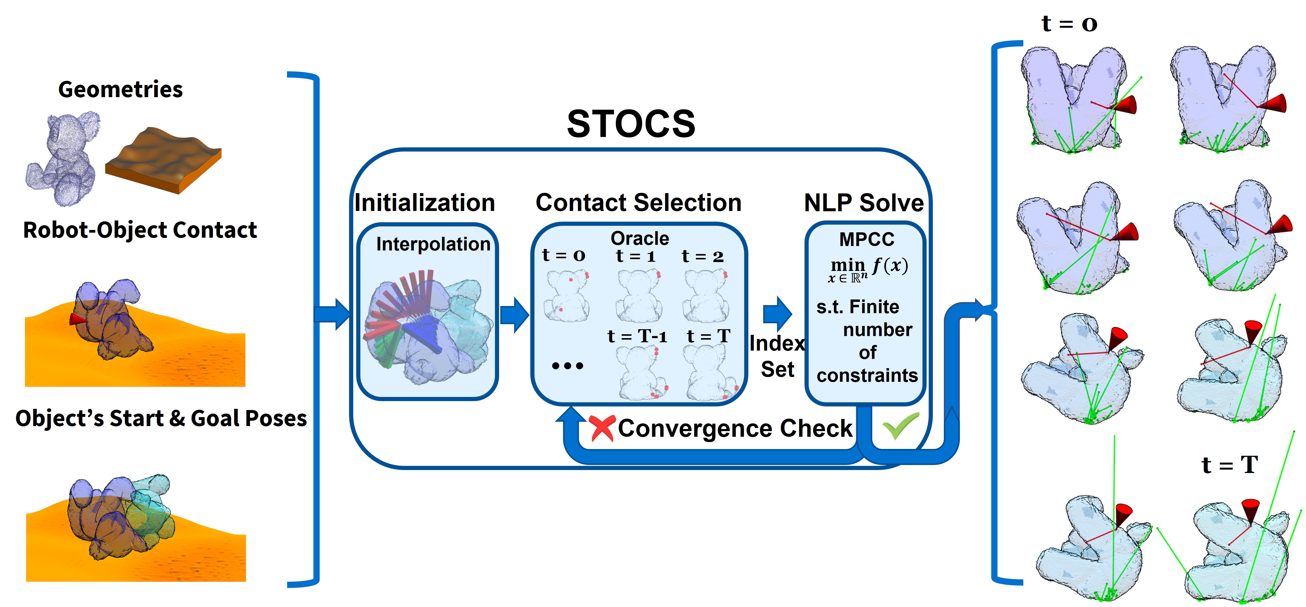
Overall, STOCS formulates contact-rich trajectory optimization as an infinite program (IP), which is a constrained optimization with a potentially infinite set of variables and constraints. It uses an exchange method to solve the IP, by wrapping a contact selection outer loop around a finite optimization problem. The inner problem formulates CITO with complementarity constraints and solves an MPCC. In summary, the algorithm operates as follows:
-
1.
Initialize the initial guess object trajectory, e.g., a linear interpolation.
-
2.
Initialize an empty candidate set of contact points for each time step and an empty set of contact forces.
-
3.
Use an Oracle to identify new / removed contact points, and update .
-
4.
Solve an MPCC for the candidate set of contact points using a small number of iterations.
-
5.
Check for convergence. If not converged, repeat from step 3.
Contact forces for existing contact points are maintained from iteration to iteration to warm-start the next MPCC. Details about the algorithm (Alg. 1) and oracle design are described below.
Infinite programming for contact-rich trajectory optimization. First, we describe the IP formulation used by STOCS. Let us start by defining semi-infinite programming (SIP). An SIP problem is an optimization problem in finitely many variables on a feasible set described by infinitely many constraints:
| (1a) | ||||
| s.t. | (1b) | |||
where is the constraint function, denotes the index parameter, and is the index domain which can be continuously infinite.
As an example, to solve pose optimization with non-penetration constraints [22], describes the pose of the object, and is a point on the surface of the object , where denotes the surface of . The constraint is the signed distance from a point to the environment. Although the inequality must be satisfied for all , optimal solutions will be supported by some points, i.e., at the optimal solution , the Karush-Kuhn-Tucker conditions will be established by a finite set of points such that .
In trajectory optimization, constraints need to be enforced in space-time [22], so we define a candidate index point as being indexed by time. We denote as the index domain at time .
STOCS then reasons about contact forces at each index point, and since the contact force distribution is a function over the object surface, this introduces infinitely many variables, which turns the problem into an infinite program [23]. Specifically, we define the contact force as an optimization variable. Our formulation imposes friction constraints, complementarity constraints, and quasi-dynamic/quasi-static force and moment balance on these variables.
To formulate the force variables and friction cone, we encode normal and tangential forces separately in the vector . In 2D, is expressed in a reference frame with the component of force normal to the contact surface, and , tangent to the contact surface. In 3D, following [5], we use a polyhedral approximation of the friction cone [24]. We express in a reference frame with normal to the contact surface, and tangent to the contact surface. The convex hull of the unit vectors along the directions of in forms the polyhedral approximation. The force is required to satisfy and where is the friction coefficient of the given point and the right hand side is the sum of tangential forces.
In summary, the constraints we impose at time are as follows:
-
1.
State and Control Bounds:
(2) -
2.
Object Dynamics:
(3) -
3.
Distance Complementarity: ensures that nonzero forces are only exerted at points where objects are in contact, i.e. the normal force is nonzero only if contact is made at .
(4) -
4.
Unilateral Manipulation Velocity: ensures the manipulator can only push the object rather than pull.
(5) -
5.
Force-torque Balance:
(6) -
6.
Friction constraints: the force constraints defined above are grouped into a function
(7) A similar constraint is applied to the manipulator contact force.
-
7.
Friction-Velocity Complementarity: ensures the relative tangential velocity at a contact is zero unless the contact force is at the boundary of the friction cone
(8)
We elaborate a bit on (6), which integrates the force distribution over the domain . Here, represents the force and torque applied by gravity and the manipulator, and represents the force and torque applied on an index point by the contact force . The integral gives the net force and torque experienced by the object, which is if we assume quasi-static, and is if we assume quasi-dynamic, where is the inertia matrix of , and is approximated as .
Lastly, adding terminal constraints and , we formulate the following infinite programming with complementarity constraints trajectory optimization (IPCC-TO) problem:
| (9a) | ||||
| s.t. | (9b) | |||
| (9c) | ||||
| (9d) | ||||
where , , and concatenate the state and control variables along all time steps, and represents the contact force distribution at all points in time. Detailed instantiations of Equation 9 for both 2D and 3D scenarios are available in the Appendix. We denote this problem as .
Exchange method. The IPCC-TO problem not only has infinitely many constraints, but also an infinity of variables in . To solve it using numerical methods, we require that only is non-zero at a finite number of points. Indeed, if an optimal solution is supported by a finite subset of index points , then it suffices to solve for the values of at these supporting points, since should elsewhere be zero thanks to (4). This concept is used in the exchange method to solve SIP problems [25], and we extend it to solve IPCC-TO.
The exchange method progressively instantiates finite index sets and their corresponding finite-dimensional MPCCs whose solutions converge toward the true optimum [26]. The solving process can be viewed as a bi-level optimization. In the outer loop, index points are selected by an oracle to be added to the index set , and then in the inner loop, the optimization is solved. The outer loop will then decide how much should move toward the solution of . Specifically, if we let be the optimal solution to , then as grows denser, the iterates of (, ) will eventually approach an optimum of .
Given a finite number of instantiated contact points , we can solve a discretized version of the problem which only creates constraints and variables corresponding to . Also, through replacing the distribution of with Dirac impulses, integrals are replaced with sums and we formulate the finite MPCC problem in the following form:
| (10a) | ||||
| s.t. | (10b) | |||
| (10c) | ||||
| (10d) | ||||
| (10e) | ||||
where , and .
Oracle. Identifying an effective selection strategy for index points is a key to solving the IPs, and this strategy is denoted the Oracle. A naive Oracle would sample index points incrementally from (e.g., randomly or on a grid) at each of the discretized time steps along the trajectory, and hopefully, with a sufficiently dense set of points the iterates of solutions will eventually approach an optimum. However, this approach is inefficient, as most new index points will not yield active contact forces during the iteration. Better strategies seek to identify a small number of points that would be active at an optimal solution. This work introduces two different Oracle designs, the Maximum Violation Oracle (MVO) and the Time-active Maximum Violation Oracle (TAMVO), which will be discussed in more detail in Sec. III-C.
Merit function for the outer iteration. After solving in an outer iteration, we get a step direction from the current iterate (, ) toward (, ), where is a concatenation of all the optimization variables except for . However, due to nonlinearity, the full step may lead to a worse constraint violation for the original problem . To avoid this, we perform a line search over the following merit function that balances reducing the objective and reducing the constraint error on the infinite dimensional problem :
| (11) |
where denotes the vector of constraint violations of Problem (9). Also, in SIP for collision geometries, a serious problem is that using existing instantiated index parameters, a step may go too far into areas where the minimum of the distance function greatly violates the inequality, and the optimization loses reliability. So we add the max-violation to , in which we denote the negative component of a term as .
Convergence criteria. We denote the index set instantiated at the outer iteration as , the corresponding MPCC as , and the solved solution as (, ).
The convergence condition is defined as and and (or ) and , where is the dimension of the optimization variable and is the number of complementarity constraints, is the step size tolerance, is the complementarity gap tolerance, is the balance tolerance, and is the penetration tolerance. With a little abuse of notation, is the concatenation of the function value of all the points in , and similar for and . is the concatenation of all the for .
III-C Oracle Choice
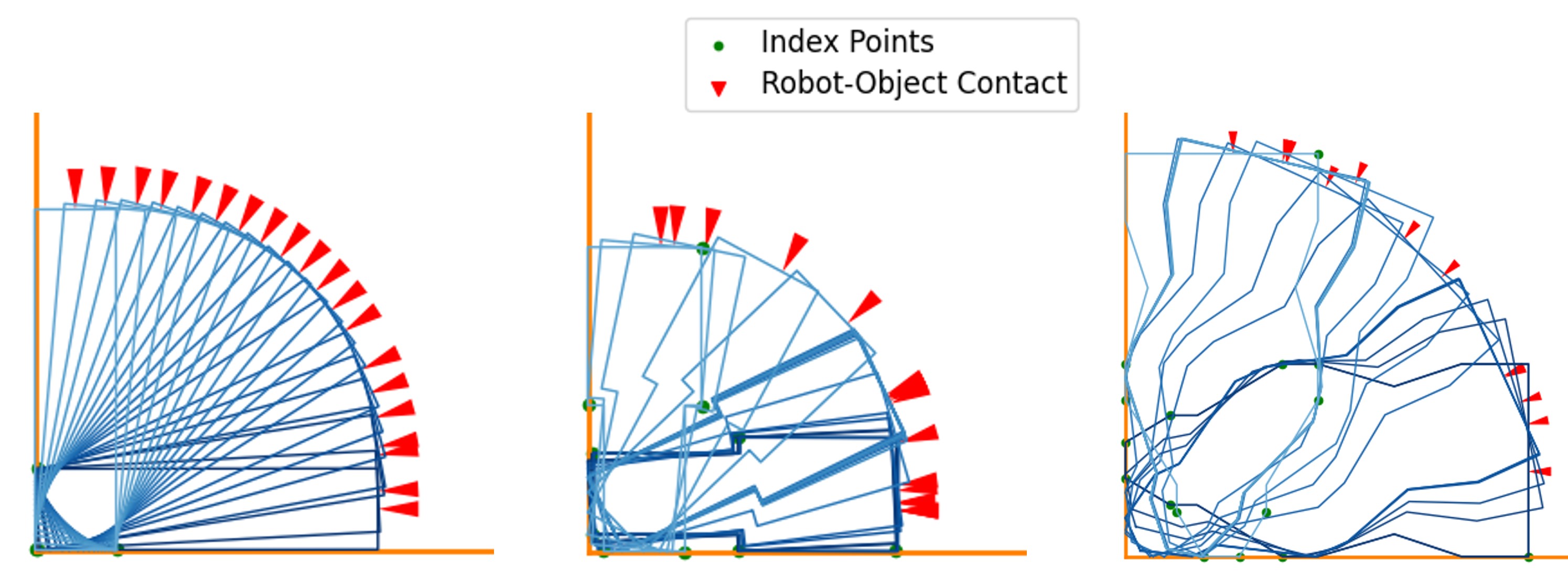
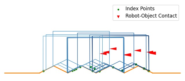
As described above, the oracle design is a key component of STOCS. We compare Maximum Violation Oracle (MVO), that adds the closest / deepest penetrating points between the object and the environment at each time step along the trajectory, along with a new method, Time Active Maximum Violation Oracle (TAMVO) with smoothing. TAMVO selects index points more judiciously and only adds the closest / deepest penetrating points at a specific time step.
MVO (Alg. 2) adds the closest or deepest penetrating points between the object and environment at each time step along the trajectory to all candidate index points across time s. Note, however, that it may still include index points that do not generate active contact forces during the iteration. For instance, as illustrated in Fig. 2(a), the closest or deepest penetrating points at time step are typically active only around that specific period.
To address this issue, we introduce TAMVO (Alg. 3). In this refined approach, the index set is no longer the same across time steps. Lines 8–12 identify closest points at each time step. Duplicate points (within threshold ) are excluded in lines 13–18. Given default parameters and , adds only the closest or most deeply penetrating points at the current time step to .

(a) Closest point on the object to the environment at each time step

(b) Index points selected by MVO at each time step

(c) Index points selected by TAMVO without SD and TS at each time step

(d) Index points selected by TAMVO with TS () at each time step

(e) Spatial Disturbance
Choosing only the closest points at the current iterate is potentially not the most ideal choice unless the current iterate is near-optimal. A better choice would anticipate which points are active at the optimum. To address this, we introduce the following two strategies designed to mitigate this issue.
Spatial Disturbance (SD). Recognizing that the current iterate is likely to be in the neighborhood of the optimal solution, the SD approach introduces perturbations to the current solution to add new candidate contact points. Consequently, in lines 9–12 of Alg. 3, is perturbed with disturbance to choose closest points. We choose to perturb along each dimension of in both positive and negative directions. In 3D, this strategy chooses 12 perturbations accounting for both increases and decreases in , , and , , . An illustration of adding perturbation to rotation in 2D is shown in Fig. 2(e).
Time Smoothing (TS). Considering that the closest points may be active not just at the current time step , but also during a surrounding interval, in line 14 of Alg. 3, the closest points detected within the adjacent time steps from to , governed by a parameter , are added to the index set of time step . The effect of using TS is illustrated in Fig. 2(d).
IV Experimental Results
The proposed methods are implemented in Python using the optimization interface and the SNOPT solver [27] provided by Drake [28].
IV-A Experiments in 2D
First, we compare STOCS with vanilla MPCC to evaluate the efficacy of dynamic contact selection on an object pivoting task. We finely discretize the object geometries to better illustrate the advantages of our method. Vanilla MPCC involves adding all index points in to an MPCC problem without selection, resulting in a larger optimization problem than in STOCS. MVO is employed in this experiment, and , , and are used for this set of the experiments.
The results are presented in Table I. We observe that STOCS can be around two to three orders of magnitude faster than MPCC, and can solve problems that MPCC cannot solve. STOCS selects only a small amount of points from the total number of points in the objects’ representation on average, which greatly decreases the dimension of the instantiated optimization problem and reduces solve time. The solved trajectories of STOCS for three different object are shown in 3.
| STOCS | MPCC | ||||
|---|---|---|---|---|---|
| Object | # Points | Time (s) | Outer iters. | Index points | Time (s) |
| Box | 212 | 4.3 | 2 | 2.0 | 2908.5 |
| Peg | 214 | 45.2 | 5 | 4.2 | 5503.9 |
| Mustard | 400 | 33.6 | 5 | 6.8 | Failed |
Next, we evaluate STOCS in a 2D setting with TAMVO, focusing on testing its applicability with objects and environments whose geometries are significantly more complex than those presented in the examples of [20]. In this experiment, we set and as the parameters for TAMVO, and we designate these as the default values for TS and SD separately. Four tasks are designed for this evaluation: pushing a dented object across uneven terrain, inserting a tilted peg into a correspondingly angled hole, and maneuvering a bean-shaped object across two distinct curvilinear terrains. The trajectories planned for these tasks are depicted in Fig. 4, and the detailed information regarding the objects’ geometries and the solve of the trajectories are presented in Table II.
, , and are used for this set of the experiments in 2D.
Same as before, STOCS selects only a small number of points from the entire set in the object’s representation to establish a solution. Typically, STOCS reaches convergence after just a few iterations. The final example, sliding the bean along curve 2, demands additional iterations and time for convergence due to the curve’s curvature shifting from concave to convex. This alteration results in different contact points at different stages along the trajectory, which takes more iterations to be fully instantiated.
(a) Pushing a dented object on uneven terrain

(b) Pushing a tilted peg into angled hole

(c) Sliding bean on curve 1

(d) Sliding bean on curve 2
| Environment | Object | # Point | Outer iters. | Index points | Time (s) |
|---|---|---|---|---|---|
| Uneven | Dented | 543 | 4 | 9.05 | 30.83 |
| Tilted Hole | Tilted Peg | 214 | 4 | 12.93 | 40.11 |
| Curve 1 | Bean | 100 | 7 | 9.43 | 72.74 |
| Curve 2 | 14 | 14.29 | 636.89 |
IV-B Experiments in 3D
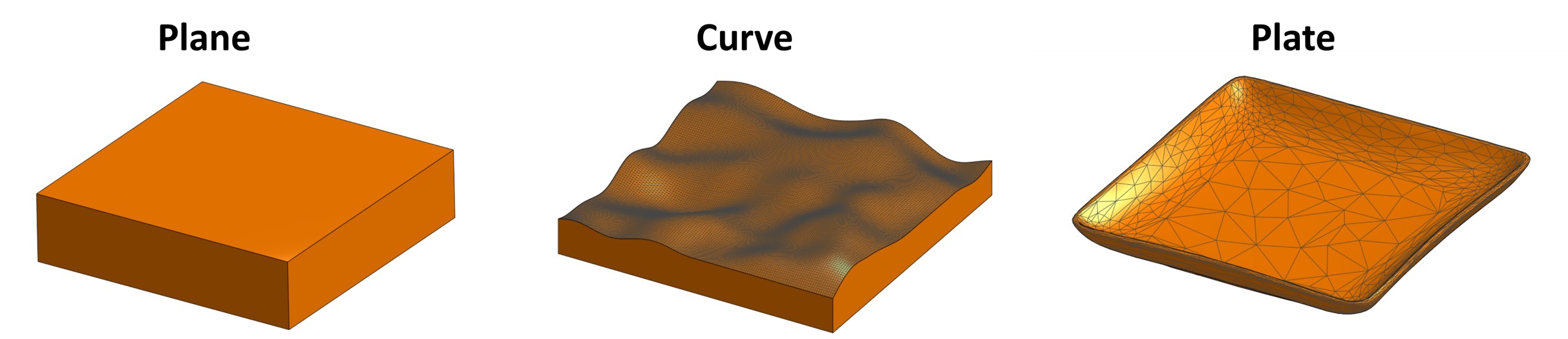
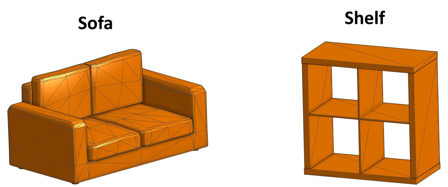
Next, we evaluate STOCS in 3D. To demonstrate its generalizability, we collect object geometries from the YCB dataset [29], the Google Scanned Objects [30], and 3D models found online [31, 32]. All the objects used in the study are shown in Fig. 5, and all the environments used in the study are shown in Fig. 6. Klampt [33] and the code in [22] are used to find the closest points between two complex shaped geometries.
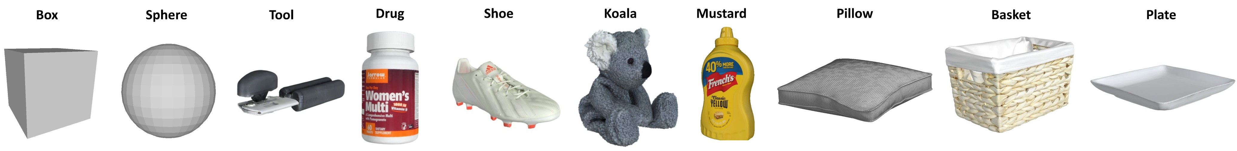
(a) Objects

(b) Point Clouds
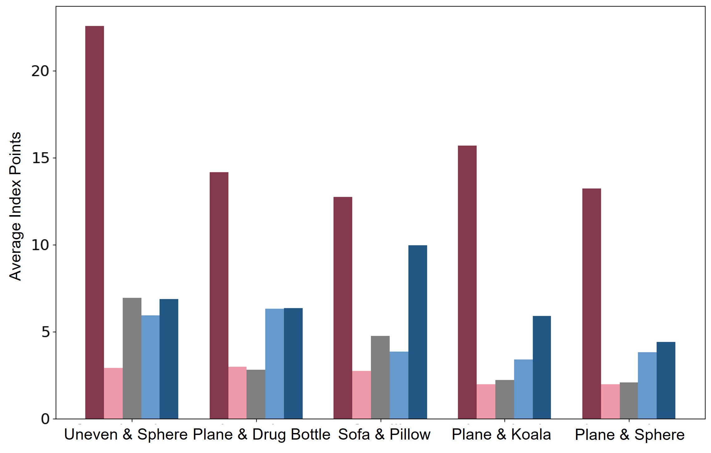
(a) Average Index Points

(b) Solve Time
As demonstrated in the first set of experiments, employing a vanilla MPCC approach by incorporating all index points in into an MPCC problem without selection results in a large optimization problem. Such an approach can take a long time to find a solution. Consequently, we have opted not to pursue experiments with the vanilla MPCC in this study, given that the 3D point clouds utilized herein contain thousands of points on average. Additionally, approximating the friction cone with a polyhedral model in a 3D context further increases the number of constraints for each index point, exacerbating the complexity beyond that encountered in 2D scenarios.
 |
 |
 |
| (a) Shoe Pushing on Plane | (b) Box Pushing on Plane | (c) Koala Pivoting on Plane |
 |
 |
 |
| (d) Mustard Pivoting on Plane | (e) Sphere Rolling on Plane | (f) Tool Rotating on Plane |
 |
 |
 |
| (g) Drug Bottle Rolling on Plane | (h) Koala Pivoting on Curved Surface | (i) Sphere Rolling on Curved Surface |
 |
 |
 |
| (j) Pillow Pivoting on Sofa | (k) Basket Pushing on Shelf | (l) Plate Sliding on Plate |
To demonstrate the effectiveness of STOCS in planning with high-fidelity geometric representations, we conduct experiments on ten different objects represented by dense point clouds sampled on the surface of the objects’ meshes, and five different environments represented by Signed Distance Field (SDF). The SDFs are calculated offline on a grid that encloses the corresponding environment given a closed polygonal mesh of the environment, and values off of the grid vertices are approximated via trilinear interpolation.
Using STOCS, we plan for pushing, pivoting, rolling and rotating trajectories on these objects. The resulting planned trajectories are illustrated in Fig. 9, while detailed information regarding the objects’ geometries and the solve of the trajectories are presented in Table III. Like the experiment in 2D, we set and as the default parameters for TAMVO. , and are used for all the experiments in 3D. For all experiments, is used except in the tasks of pushing a basket on a shelf and sliding a plate on another plate, where is used. To model the robot manipulatior as having a patch contact, 3 to 5 object vertices in the neighborhood of the indicated cone are allowed to be used as contact points.
| Environment | Object | Task | # Point | Outer iters. | Index points | Time (s) |
| Plane | Box | Push | 764 | 3 | 5.75 | 24.84 |
| Shoe | Push | 17890 | 6 | 4.95 | 144.71 | |
| Koala | Pivot | 67359 | 4 | 5.89 | 37.93 | |
| Mustard | Pivot | 8424 | 3 | 8.58 | 59.37 | |
| Sphere | Roll | 2362 | 6 | 4.39 | 94.42 | |
| Tool | Rotate | 8316 | 6 | 5.09 | 99.85 | |
| Drug | Roll | 5533 | 10 | 6.35 | 319.72 | |
| Curve | Koala | Pivot | 67359 | 9 | 13.47 | 676.01 |
| Sphere | Roll | 2362 | 4 | 6.86 | 72.66 | |
| Sofa | Pillow | Pivot | 13316 | 7 | 9.95 | 201.39 |
| Shelf | Basket | Push | 71961 | 7 | 23.10 | 421.30 |
| Plate | Plate | Slide | 67283 | 3 | 24.67 | 54.02 |
Following the initial assessments, we further evaluated the efficacy of the TAMVO alongside the SD and TS techniques through a set of comparative experiments. These experiments utilized STOCS to plan trajectories for the same set of tasks, with the primary variation being the specific oracle employed in each scenario.
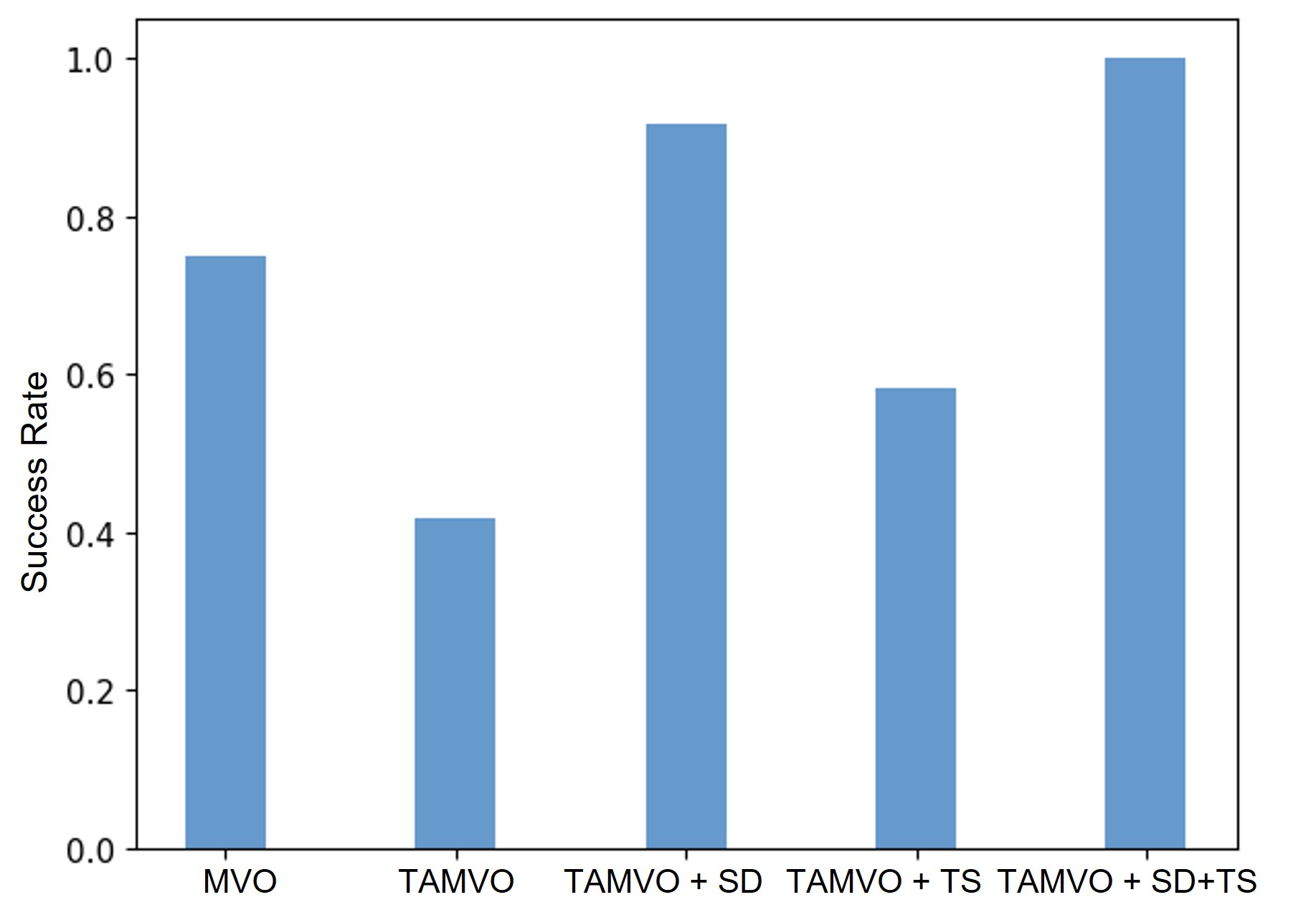
Figure 7 presents the success rates of all tested Oracles. The data shows that the MVO achieves a success rate. In contrast, TAMVO without SD and TS exhibits worse performance than MVO; this is particularly evident in 3D scenarios where relying solely on the nearest object-to-environment point is inadequate for fulfilling the object’s balance constraints. The SD and TS techniques, introduced to address this challenge, both demonstrated enhanced performance when combined with TAMVO, surpassing the success rate of TAMVO alone. Furthermore, the integration of SD and TS with TAMVO consistently achieved successful trajectory planning for all tasks.
Figure 8 displays the average number of index points selected at each time step by the different Oracles assessed in our study, focusing on tasks that were successfully solved by all Oracles. As depicted in Fig. 8(a), the MVO selects a larger number of points than TAMVO and all its variations. Notably, TAMVO combined with SD and TS can successfully plan trajectories for all tasks while selecting fewer index points compared to MVO. These findings validate our hypothesis regarding TAMVO: an index point identified at time step is most valuable within a temporal vicinity of . Furthermore, these results substantiate our rationale for introducing SD and TS, affirming that a localized exploration in both temporal and spatial dimensions offers a more efficient strategy than incorporating index points identified at distant time steps along the trajectory.
Figure 8(b) presents the solve times for STOCS employing various Oracles across all successful tasks. The results indicate that the quantity of index points selected by an Oracle does not necessarily correlate with the solve time. For instance, in the sphere rolling on plane task, TAMVO+SD+TS chooses a larger number of index points than TAMVO+TS, yet the solve time for TAMVO+SD+TS is much faster than that of TAMVO+TS. Similarly, in the case of the drug bottle rolling on plane task, it can be seen that both TAMVO+SD+TS and TAMVO+TS select a comparable number of index points, yet the solve time for TAMVO+TS is much faster than TAMVO+SD+TS. This phenomenon underscores that a larger number of index points does not invariably lead to longer solve time. Although TAMVO+SD+TS provides the best performance in terms of success rate, it is not guaranteed to give the best solve time for all different tasks.
V Conclusion and Discussion
This paper introduces Simultaneous Trajectory Optimization and Contact Selection (STOCS) to address the scaling problem in contact-implicit trajectory optimization (CITO). Through embedding CITO in an infinite programming (IP) framework to dynamically instantiate possible contact points and contact times between the object and environment inside the optimization loop, STOCS entends the application of CITO to a much higher number of contact points. The introduction of the Time-Active Maximum Violation Oracle along with Spatial Disturbance and Temporal Smoothing techniques for more efficient index point selection further enables STOCS to plan contact-rich manipulation trajectories with dense point clouds representation of complex-shaped objects. To the best of our knowledge, this is the first method capable of planning contact-rich manipulation trajectories with high-fidelity geometric representations in 3D.
Looking ahead, to further facilitate the practical application of the STOCS algorithm to raw object point clouds obtained from RGB-D sensors, it will be essential to devise effective pre-processing techniques for the point cloud data. This is crucial given that raw depth data typically contain a significant amount of noise. Moreover, STOCS presupposes the knowledge of specific physical properties of the object, such as mass, center of mass, and friction coefficients. However, accurately measuring these parameters in practice can be challenging, and discrepancies between the nominal values used during planning and their actual real-world counterparts may lead to failures in execution. It would be of considerable interest to explore the incorporation of robust optimization techniques into the STOCS framework to develop manipulation trajectories that maintain robustness against uncertainty in physical parameters.
Acknowledgments
This paper is partially supported by NSF Grant #IIS-1911087.
References
- [1] M. Dogar, K. Hsiao, M. Ciocarlie, and S. Srinivasa, Physics-based grasp planning through clutter. MIT Press, 2012.
- [2] C. Eppner and O. Brock, “Planning grasp strategies that exploit environmental constraints,” in 2015 IEEE international conference on robotics and automation (ICRA). IEEE, 2015, pp. 4947–4952.
- [3] M. Kelly, “An introduction to trajectory optimization: How to do your own direct collocation,” SIAM Review, vol. 59, no. 4, pp. 849–904, 2017.
- [4] G. Schultz and K. Mombaur, “Modeling and optimal control of human-like running,” IEEE/ASME Transactions on mechatronics, vol. 15, no. 5, pp. 783–792, 2009.
- [5] M. Posa, C. Cantu, and R. Tedrake, “A direct method for trajectory optimization of rigid bodies through contact,” The International Journal of Robotics Research, vol. 33, no. 1, pp. 69–81, 2014.
- [6] I. Mordatch, Z. Popović, and E. Todorov, “Contact-invariant optimization for hand manipulation,” in Proceedings of the ACM SIGGRAPH/Eurographics Symposium on Computer Animation, 2012, pp. 137–144.
- [7] I. Mordatch, E. Todorov, and Z. Popović, “Discovery of complex behaviors through contact-invariant optimization,” ACM Transactions on Graphics (TOG), vol. 31, no. 4, pp. 1–8, 2012.
- [8] A. Patel, S. L. Shield, S. Kazi, A. M. Johnson, and L. T. Biegler, “Contact-implicit trajectory optimization using orthogonal collocation,” IEEE Robotics and Automation Letters, vol. 4, no. 2, pp. 2242–2249, 2019.
- [9] A. Ö. Önol, R. Corcodel, P. Long, and T. Padır, “Tuning-free contact-implicit trajectory optimization,” in 2020 IEEE International Conference on Robotics and Automation (ICRA). IEEE, 2020, pp. 1183–1189.
- [10] Z.-Q. Luo, J.-S. Pang, and D. Ralph, Mathematical programs with equilibrium constraints. Cambridge University Press, 1996.
- [11] M. Zhang and K. Hauser, “Semi-infinite programming with complementarity constraints for pose optimization with pervasive contact,” in 2021 IEEE International Conference on Robotics and Automation (ICRA). IEEE, 2021, pp. 6329–6335.
- [12] F. H. Clarke, Optimization and nonsmooth analysis. SIAM, 1990.
- [13] K. Harada, K. Hauser, T. Bretl, and J.-C. Latombe, “Natural motion generation for humanoid robots,” in 2006 IEEE/RSJ International Conference on Intelligent Robots and Systems. IEEE, 2006, pp. 833–839.
- [14] N. Chavan-Dafle, R. Holladay, and A. Rodriguez, “Planar in-hand manipulation via motion cones,” The International Journal of Robotics Research, vol. 39, no. 2-3, pp. 163–182, 2020.
- [15] Y. Shirai, D. K. Jha, A. U. Raghunathan, and D. Romeres, “Robust pivoting: Exploiting frictional stability using bilevel optimization,” in 2022 International Conference on Robotics and Automation (ICRA). IEEE, 2022, pp. 992–998.
- [16] X. Cheng, E. Huang, Y. Hou, and M. T. Mason, “Contact mode guided sampling-based planning for quasistatic dexterous manipulation in 2d,” in 2021 IEEE International Conference on Robotics and Automation (ICRA). IEEE, 2021, pp. 6520–6526.
- [17] ——, “Contact mode guided motion planning for quasidynamic dexterous manipulation in 3d,” in 2022 International Conference on Robotics and Automation (ICRA). IEEE, 2022, pp. 2730–2736.
- [18] E. Huang, X. Cheng, and M. T. Mason, “Efficient contact mode enumeration in 3d,” in International Workshop on the Algorithmic Foundations of Robotics. Springer, 2021, pp. 485–501.
- [19] M. Zhang and K. Hauser, “Semi-infinite programming with complementarity constraints for pose optimization with pervasive contact,” May 2021.
- [20] M. Zhang, D. K. Jha, A. U. Raghunathan, and K. Hauser, “Simultaneous trajectory optimization and contact selection for multi-modal manipulation planning,” arXiv preprint arXiv:2306.06465, 2023.
- [21] M. T. Mason, Mechanics of robotic manipulation. MIT press, 2001.
- [22] K. Hauser, “Semi-infinite programming for trajectory optimization with non-convex obstacles,” The International Journal of Robotics Research, vol. 40, no. 10-11, pp. 1106–1122, 2021.
- [23] E. J. Anderson and A. B. Philpott, Infinite Programming: Proceedings of an International Symposium on Infinite Dimensional Linear Programming Churchill College, Cambridge, United Kingdom, September 7–10, 1984. Springer Science & Business Media, 2012, vol. 259.
- [24] D. E. Stewart and J. C. Trinkle, “An implicit time-stepping scheme for rigid body dynamics with inelastic collisions and coulomb friction,” International Journal for Numerical Methods in Engineering, vol. 39, no. 15, pp. 2673–2691, 1996.
- [25] M. López and G. Still, “Semi-infinite programming,” European Journal of Operational Research, vol. 180, no. 2, pp. 491–518, 2007.
- [26] R. Reemtsen and S. Görner, “Numerical methods for semi-infinite programming: a survey,” in Semi-Infinite Programming. Springer, 1998, pp. 195–275.
- [27] P. E. Gill, W. Murray, and M. A. Saunders, “Snopt: An sqp algorithm for large-scale constrained optimization,” SIAM review, vol. 47, no. 1, pp. 99–131, 2005.
- [28] R. Tedrake and the Drake Development Team, “Drake: Model-based design and verification for robotics,” 2019. [Online]. Available: https://drake.mit.edu
- [29] B. Calli, A. Walsman, A. Singh, S. Srinivasa, P. Abbeel, and A. M. Dollar, “Benchmarking in manipulation research: The ycb object and model set and benchmarking protocols,” arXiv preprint arXiv:1502.03143, 2015.
- [30] L. Downs, A. Francis, N. Koenig, B. Kinman, R. Hickman, K. Reymann, T. B. McHugh, and V. Vanhoucke, “Google scanned objects: A high-quality dataset of 3d scanned household items,” in 2022 International Conference on Robotics and Automation (ICRA). IEEE, 2022, pp. 2553–2560.
- [31] Open Robotics. [Online]. Available: https://app.gazebosim.org/OpenRobotics/fuel/models/Sofa
- [32] Sketchfab. [Online]. Available: https://sketchfab.com/3d-models/burlap-pillow-1ef567278bba4db68ac5488d6b4bc851
- [33] Klampt – Intelligent Motion Laboratory at UIUC. [Online]. Available: http://motion.cs.illinois.edu/klampt/
Appendix
We discuss the detailed instantiation of the MPCC problem that needs to be solved inside STOCS for both 2D and 3D scenarios separately.
V-A 2D
V-A1 Geometry modeling
To handle collision avoidance, we establish a semi-infinite constraint between the object and the environment. The object is represented as a densely sampled point cloud on its surface, and the environment is represented as a signed distance field (SDF) which supports depth lookup. Specifically, we define with the object transform at configuration .
V-A2 Friction force modeling
The force variable of the index point at time step is , which is divided into the normal component and frictional components and along the tangential direction of the contact surface [24]. Given the normal vector along the outward surface normal of the environment, and and , the overall force applied at index point is . Each of the components of is required to be non-negative, and given the friction coefficient , the friction cone constraint is given by .
Similarly, for the contact between the robot and the object, we define the force variable at time step to be . Besides, the normal vector along the inward surface normal of the object, and the tangential vectors and which are perpendicular to the normal vector are defined in the object’s local frame.
We adopt a heuristic to reduce the number of constraints in the complementarity condition and accelerate solve times. By only applying complementarity to the normal component of force variables, , we reduce the number of distance complementarity constraints from to , and the problem is unchanged because due to the friction cone constraint.
V-A3 Force and torque balance
We establish an equality constraint on the object’s force and torque balance. It requires the joint force and torque exerted by the robot, the environment, and the gravity on the object to be if we assume quasistatic, and to be if we assume quasidynamic, where is the inertia matrix of the object and is the velocity of the object.
V-A4 Instantiation of MPCC problem
With these definitions, the nonlinear programming problem that needs to be solved at the iteration of STOCS is the following:
| (12a) | ||||
| (12b) | ||||
| (12c) | ||||
| (12d) | ||||
| (12e) | ||||
| (12f) | ||||
| (12g) | ||||
| (12h) | ||||
| (12i) | ||||
| (12j) | ||||
| (12k) | ||||
| (12l) | ||||
| (12m) | ||||
| (12n) | ||||
| (12o) | ||||
| (12p) | ||||
where , , is the relative tangential velocity at contact point . , is the contact point between the robot and the object in the object’s frame, is the center of mass of the object, is the translational velocity of the object, is the translational part of the inertia matrix of the object with appropriate dimension, and and are the corresponding terms for the rotational part.
V-B 3D
V-B1 Geometry modeling
To handle collision avoidance, like in the 2D scenario, we establish a semi-infinite constraint between the object and the environment. The object is represented as a densely sampled point cloud on its surface, and the environment is represented as a signed distance field (SDF) which supports depth lookup. We define with the object transform at configuration .
V-B2 Friction force modeling
In 3D scenario, following [5], to preserve the MPCC structure of the resulting optimization problem, we use a polyhedral approximation of the friction cone [24]. The force variable of the index point at time step is , which is expressed in a reference frame with normal to the contact surface, and tangent to the contact surface. The convex hull of the unit vectors along the directions of in forms the polyhedral approximation. The normal vector is along the outward surface normal of the environment, and are perpendicular to . Each of the components of is required to be non-negative, and given the friction coefficient , the friction cone constraint is given by .
Similarly, for the contact between the robot and the object, we define the force variable at time step to be . The normal vector is along the inward surface normal of the object, and are perpendicular to .
The same heuristic is used to reduce the number of constraints in the complementarity condition and accelerate solve times. By only applying complementarity to the normal component of force variables, , we reduce the number of distance complementarity constraints from to , and the problem is unchanged because due to the friction cone constraint.
V-B3 Instantiation of MPCC problem
With these definitions the nonlinear programming problem that needs to be solved at the iteration for this pivoting task is the following:
| (13a) | ||||
| (13b) | ||||
| (13c) | ||||
| (13d) | ||||
| (13e) | ||||
| (13f) | ||||
| (13g) | ||||
| (13h) | ||||
| (13i) | ||||
| (13j) | ||||
| (13k) | ||||
| (13l) | ||||
| (13m) | ||||
| (13n) | ||||
| (13o) | ||||
where , , is the relative tangential velocity at contact point . , is the contact point between the robot and the object in the object’s frame, is the center of mass of the object, is the translational velocity of the object, is the translational part of the inertia matrix of the object with appropriate dimension, and and are the corresponding terms for the rotational part.