Simultaneous Shape and Mesh Quality Optimization using Pre-Shape Calculus
Abstract
Computational meshes arising from shape optimization routines commonly suffer from decrease of mesh quality or even destruction of the mesh. In this work, we provide an approach to regularize general shape optimization problems to increase both shape and volume mesh quality. For this, we employ pre-shape calculus as established in [12]. Existence of regularized solutions is guaranteed. Further, consistency of modified pre-shape gradient systems is established. We present pre-shape gradient system modifications, which permit simultaneous shape optimization with mesh quality improvement. Optimal shapes to the original problem are left invariant under regularization. The computational burden of our approach is limited, since additional solution of possibly larger (non-)linear systems for regularized shape gradients is not necessary. We implement and compare pre-shape gradient regularization approaches for a hard to solve 2D problem. As our approach does not depend on the choice of metrics representing shape gradients, we employ and compare several different metrics.
Key words: Shape Optimization, Mesh Quality, Mesh Deformation Method, Shape Calculus
AMS subject classifications: 49Q10, 65M50, 90C48, 49J27
1 Introduction
Solutions of PDE constrained optimization problems, in particular problems where the desired control variable is a geometric shape, are only meaningful, if the state variables of the constraint can be calculated with sufficient reliability. A key component of reliable solutions is given by the quality of the computational mesh. It is well-known that poor quality of elements affect the stability, convergence, and accuracy of finite element and other solvers. This comes from effects such as poorly conditioned stiffness matrices (cf. [19]).
There are a multitude of strategies for increasing mesh quality, particularly in shape optimization. The authors of [5] enhance mesh morphing routines for shape optimization by trying to correct for the inexactness of Hadamard’s theorem due to discretization of the problem. Correcting degenerate steps requires a restriction of deformation directions based on normal fields of shapes, which leads to a linear system enlarged by additional constraints. In [9], an approach to shape optimization using the method of mappings to guarantee non-degenerate deformations of meshes is presented. For this, the shape optimization problem is regarded as an optimization in function spaces. A penalty term for the Jacobian determinants of the deformations is added, which leads to a non-smooth optimality system. Deformations computed by solving this system have less tendency to degenerate volumes of cells. These techniques are related to the techniques of our work, however they do not include a mechanism to capture a target mesh volume distribution as is presented here in subsequent sections. In [14] metrics for representing shape gradients are modified by adding a non-linear advection term. For this, the shape derivative is represented on the shape seen as a boundary mesh, which is then used as a Neumann condition to assemble a system incorporating the non-linear advection term to represent a shape gradient in volume formulation. This formulation advects nodes of the volume mesh in order to mitigate element degeneration, but requires solution of a non-linear system to construct the shape gradient. In [16], the author applies mesh smoothing inspired by centroidal Voronoi reparameterization to construct a tangential field that corrects for degenerate surface mesh cells. For correcting the volume mesh cell degeneration, a shape gradient representation featuring a non-linear advection term is used. This is motivated by the eikonal equation, while orthogonality of the correction to shape gradients is ensured by a Neumann condition. In order to mitigate roughness of gradients and resulting degeneration of meshes, the authors of [18] construct shape gradient representations by use of Steklov-Poincaré metrics. As an example they propose the linear elasticity metric, giving a more regular shape gradient representation by solution of a linear system using volume formulations of shape derivatives. In [10], the authors construct a Riemannian metric for the manifold of planar triangular meshes with given fixed connectivity, which makes the space geodesically complete. They propose a mesh morphing routine by geodesic flows, using the Hamiltonian formulation of the geodesic equation and solving by a symplectic numerical integrator. Numerical experiments in [10] suggest that cell aspect ratios are bounded away from zero and thus avoid mesh degradation during deformations.
Several of the aforementioned approaches require modification of the metrics acting as left hand sides to represent shape gradients. Often, either non-linear terms are added or systems are enlarged, which increases computational burden significantly. Further, the mesh quality resulting by these regularized deformations is arbitrary or of rather implicit nature, since no explicit criterion for mesh quality is enforced.
In this work, we want to approach these two aspects differently. By using pre-shape calculus techniques introduced in [12], we propose regularization techniques for shape gradients with two goals in mind. First, the required computational burden should be limited. We achieve this by modifying the right hand sides of shape gradient systems, instead of altering the metric. This ensures that shape gradient systems neither increase in size nor become non-linear. Secondly, our regularization explicitly targets mesh qualities defined by the user. To do so, we enforce surface and volume cell distribution via use of pre-shape derivatives of pre-shape parameterization tracking problems. Non-uniform node distributions according to targets can be beneficial, especially in the context of PDE constrained optimization.
In [6] local sensitivities for minimization of the approximation error of linear elliptic second order PDE are derived and used to refine computational meshes. Also, [2] studies various monitor functions (targets) for mesh deformation methods in 2D by using elliptic and eigenvalue methods, e.g. to ensure certain coordinate lines of the mesh. Amongst other examples, this shows possible demand for targeted non-uniform adaptation of computational meshes. Non-uniform cell distributions are possible with our approach our pre-shape calculus techniques enable efficient routines solving shape optimization problems, which simultaneously optimize quality of the surface mesh representing the shape and the volume mesh representing the hold-all domain. This is done in a manner that does not interfere with the original shape optimization problem, leaving optimal and intermediate shapes invariant. An complementing literature review is found in the introduction of [12]. For this work we build on results of [12], where pre-shape calculus is rigorously established. The results from [12] feature a structure theorem in the style of Hadamard’s theorem for shape derivatives, which also shows the relationship of classical shape and pre-shape derivatives. In particular, shape calculus and pre-shape differentiability results carry over to the pre-shape setting. Further, the pre-shape parameterization tracking problem is introduced in [12, Prop. 2, Thrm. 2], where existence of solutions is proved and a closed formula for its pre-shape derivative is derived.
This work is structured in 2 sections. First, in section 2 we establish theoretical results for pre-shape regularization routines for shape and volume mesh quality. In particular, section 2.1 focuses on the regularization for shape mesh quality, while section 2.2 we take care of volume mesh quality regularization for the hold-all domain. For both cases, existence results of regularized pre-shape solutions are provided. Also, regularized pre-shape gradient systems are formulated, and consistency of regularized and unregularized gradients is established. In section 3 we display our techniques for a model problem. Several different (un-)regularized routines are tested. As a standard approach, we recommend the linear elasticity metric as found in [17]. To illustrate the general applicability of our regularization method, we also test the very reasonable -Laplacian metrics as inspired by [13] to represent gradients.
2 Theoretical Aspects of Regularization by Pre-Shape Parameterization Tracking
The main goal of this paper is to introduce a regularization approach to shape optimization, which increases mesh quality during optimization at minimal additional computational cost. To achieve this, we proceed in two steps. First, in section 2.1, we analyze the case where quality of the mesh modeling a shape is optimized. This amounts to increasing quality of the (hyper-)surface shape mesh embedded in the volume hold-all domain. Then, in section 2.2, we build on the surface mesh case by also demanding to increase the volume mesh quality of the hold-all domain. Both approaches need to satisfy two properties. On the one hand, they must not interfere with the original shape optimization problem, i.e. leave the optimal shape or even intermediate shapes invariant. On the other hand, to be practically feasible, the mesh quality regularization approach should not increase computational cost. In particular, no additional solution of linear systems should be necessary if compared to standard shape gradient descent algorithms. We will achieve both properties for the case of simultaneous shape and volume mesh quality optimization.
If not stated otherwise, we assume to be an -dimensional, orientable, path-connected and compact -manifold without boundary. In light of [12], we will assume to be the space of pre-shapes and to be the space of shapes.
2.1 Simultaneous Tangential Mesh Quality and Shape Optimization
In this subsection we formulate a regularized shape optimization problem to track for desired shape mesh quality using pre-shapes calculus. As mentioned in the introduction, we heavily build on the results of [12].
2.1.1 Preliminaries for Mesh Quality Optimization using Pre-Shapes
Throughout section 2, we take a look at a general prototype shape optimization problem
| (1) |
Here we only assume that the shape functional is first order shape differentiable.
Now we reformulate eq. 1 in the context of pre-shape optimization by use of the canonical projection . The canonical projection maps each pre-shape to an equivalence class , which consists of all pre-shapes mapping onto the same image shape in . We remind the reader that we can associate with the set interpretation of the shape . So can be interpreted as the set of all parameterizations of a given shape in . The pre-shape formulation of eq. 1 takes the form
| (2) |
It is important to notice that the extended target functional of eq. 2 is pre-shape differentiable in the sense of [12, Definition 3], since we assumed to be shape differentiable (cf. [12, Prop. 1]).
Next, we need the pre-shape parameterization tracking functional introduced in [12, Prop. 2]. In the discrete setting, this functional allows us to track for given desired sizes of surface and volume mesh cells. For this, let us assume functions and to be smooth and fulfill the normalization condition
| (3) |
Further, we assume to have shape functionality (cf. [12, Definition 2]), i.e.
| (4) |
Shape functionality for simply means, that for all pre-shapes corresponding to the same shape .
Finally, the pre-shape parameterization tracking problem takes the form
| (5) |
where is the covariant derivative. For each shape there exists a pre-shape minimizing eq. 5, which is guaranteed by [12, Prop. 2].
As we need the pre-shape derivative of the parameterization tracking functional in order to devise our algorithms, we state it in the style of the pre-shape derivative structure theorem [12, Thrm. 1]
| (6) |
with normal/ shape component
| (7) | ||||
and tangential/ pre-shape component
| (8) | ||||
Notice that we signify a duality pairing by , and with the classical shape derivative of in direction . For the derivation of the pre-shape derivative by use of pre-shape calculus, we refer the reader to [12, Thrm. 2, Cor. 2].
2.1.2 Regularization of Shape Optimization Problems by Shape Parameterization Tracking
All ingredients necessary are now available to formulate a regularized version of a shape optimization problem. For , we add the parameterization tracking functional in style of a regularizing term to pre-shape reformulation eq. 2
| (9) |
We already found that the pre-shape extension eq. 2 of our initial shape optimization problem is pre-shape differentiable. Hence eq. 9 is pre-shape differentiable as well. This is foundational, since a pre-shape gradient system for the regularized problem eq. 9 can always be formulated.
The pre-shape derivative of the parameterization tracking problem (cf. eq. 6) is well-defined for weakly differentiable directions . By assuming the same for the shape derivative of the original problem eq. 1, we can create a pre-shape gradient system for eq. 9 using a weak formulation with -functions. Given a symmetric, positive-definite bilinear form (e.g. [17], [13]), such a system takes the form
| (10) |
With , the right hand side of eq. 10 is indeed the full pre-shape gradient of eq. 9. This stems from the fact that the pre-shape extension has shape functionality by construction, which makes the pre-shape derivative equal to the shape derivative by application of [12, Thrm. 1 ].
The full pre-shape gradient system eq. 10 already achieves simultaneous solution of the shape optimization problem and regularization of shape mesh quality. Namely, it is not required to additionally solve linear systems to create a mesh quality regularized descent direction , since the original shape gradient system to problem eq. 1 is modified by adding the two force terms and . A calculation of a descent direction by combining the shape gradient and pre-shape gradient solving the decoupled systems
| (11) |
and
| (12) |
is in fact equivalent to solution of eq. 10.
However, by using eq. 10 for gradient based optimization, the first demanded property of leaving the optimal or intermediate shapes invariant is not true in general. This issue comes from involvement of the shape component (cf. eq. 7) of the pre-shape derivative to the parameterization tracking functional . It is acting solely in normal directions, therefore altering shapes by interfering with the shape derivative of the original problem.
For this reason, we deviate from the full gradient system eq. 10 consistent with the regularized problem eq. 9 by using a modified system
| (13) |
We project the pre-shape derivative onto its tangential part, which is realized by simply removing the shape component from the right hand side of the gradient system. By this we still have numerical feasibility, while also achieving invariance of optimal and intermediate shapes. Of course invariance is only true up to discretization errors. From a traditional shape optimization perspective, this stems from considering eq. 13 as a shape gradient system with additional force term acting on directions in the kernel of the classical shape derivative . In particular, by Hadamard’s theorem or the structure theorem for pre-shape derivatives [12, Thrm. 1], directions tangential to shapes are in the kernel of . Using the pre-shape setting, we interpret these directions as vector fields corresponding to the fiber components of .
To sum up and justify the use of the pre-shape regularized problem eq. 9 and its modified gradient system eq. 13, we provide existence of solutions and consistency of the modified gradients with the regularized problem.
Theorem 1 (Shape Regularized Problems).
Assume to be an -dimensional, orientable, path-connected and compact -manifold without boundary. Let shape optimization problem eq. 1 be shape differentiable and have a minimizer . For shape parameterization tracking, let us assume functions and to be smooth, fulfill the normalization condition eq. 3, and to have shape functionality eq. 4.
Then there exists a minimizing the shape regularized problem eq. 9.
The modified pre-shape gradient system eq. 13 is consistent with the full pre-shape gradient system eq. 10 and the shape gradient system of the original problem eq. 11, in the sense that
| (14) |
In particular, if is satisfied, the necessary first order conditions for eq. 9 and eq. 1 are satisfied as well.
Proof.
For the existence of solutions to the regularized problem eq. 9, let us assume there exists a minimizer to the original problem eq. 1. By construction of the shape space by equivalence relation there exists a , such that . So the set of pre-shapes acts as a set of candidates for solutions to eq. 9. Since we required shape functionality of and normalization condition eq. 3, the existence and characterization theorem for solutions to eq. 5 (cf. [12, Prop. 2]) gives existence of a global minimizer for in every fiber of . In particular, we can find such a in . From the last assertion of [12, Prop. 2] we also get that . However, since due to the quadratic nature of the parameterization tracking functional, we get that is a solution to the regularized problem eq. 9.
Next, we prove the non-trivial direction ’’ for consistency of gradient systems in the sense of eq. 14. Let us assume we have a pre-shape gradient stemming from the modified system eq. 13. This immediately gives us
| (15) |
However, due to the structure theorem for pre-shape derivatives [12, Thrm. 1], we know that the support of shape derivative and pure pre-shape component are orthogonal. Hence we have
| (16) |
This is the first order condition for eq. 1, also giving us .
It remains to show that the first order condition for the regularized problem eq. 9 is satisfied and the complete gradient . Essentially, this is a special case of result [12, Prop. 3], which characterizes global solutions of eq. 5 by fiber stationarity. From eq. 16 we see that is a fiber stationary point, since the full pre-shape derivative vanishes for all directions tangential to . Hence [12, Prop. 3] states that is already a global minimizer of and satisfies the corresponding necessary first order condition. Even more, [12, Prop. 3] gives vanishing of . Therefore the right hand side of the full gradient system eq. 10 is zero, giving us a vanishing full gradient .
Implication ’’ can be seen by the fiber stationarity characterization as well. Since vanishing of the shape gradient gives , the full pre-shape derivative must be zero if the full pre-shape gradient . Hence the fiber stationarity characterization [12, Prop. 3] tells us that both and vanish for , which proves the other direction of eq. 14. ∎
With theorem 1 we can rest assured that optimization algorithms using the tangentially regularized gradient from eq. 13 leave stationary points of the original problem invariant. Also, vanishing of the modified gradient indicates that we have a stationary shape with parameterization having desired cell volume allocation . Of course, this is only true up to discretization error. We also see that the modified gradient system eq. 13 captures the same information as the shape gradient system eq. 11 and full pre-shape gradient system eq. 10 combined. This might seem counterintuitive at first glance, especially since necessary information is contained in one instead of two gradient systems. However, by application of pre-shape calculus to derive the fiber stationarity characterization of solutions [12, Prop. 3], we recognize this circumstance as a consequence of the special structure of regularizing functional . The fact that pre-shape spaces are fiber spaces with locally orthogonal tangential bundles for parameterizations and shapes (cf. [12, Section 2]) is a fundamental prerequisite to this. We will discuss numerical results comparing optimization using standard shape gradients eq. 11 and gradients regularized by modified shape parameterization tracking eq. 13 in section 2.
Remark 1 (Applicability of Shape Regularization for General Shape Optimization Problems).
It is important to notice, that we did not need a specific structure of the original shape optimization problem eq. 1. The only assumptions made are shape differentiability and existence of an optimal shape for . This means the tangential mesh regularization via (cf. eq. 9) is applicable for almost every meaningful shape optimization problem. In particular, PDE-constrained shape optimization problems can be regularized by this approach, which we will discuss in section 3. Also, the modified gradient system structure eq. 13 stays the same for different shape optimization targets . It is solely the shape derivative on the right hand side which changes depending on the shape problem target. Finally, existence of solutions and consistency of stationarity and first order conditions theorem 1 is given
Remark 2 (Equivalent Bi-Level Formulation of the Regularized Problem).
It is also possible to formulate the shape mesh regularization as a nonlinear bilevel problem
| (17) | ||||
The upper level pre-shape optimization problem depends only on the lower level shape optimization problem by the latter restricting the set of feasible points . So intuitively, solving eq. 17 amounts to solving the lower level problem for a shape , and then to look for an optimal parameterization in the fiber corresponding to the optimal shape. If a solution to the lower level shape optimization problem exists, a solution to the upper level problem exists as well (cf. [12, Prop. 2]). The lower level problem enforces that the optimal shape coincides with the fiber .
The bilevel formulation motivates the modified gradient system eq. 13 in a consistent manner. For this, we can take the perspective of nonlinear bilevel programming as in [15]. In finite dimensions, the authors of [15] propose a way to calculate a descent direction by solving a bilevel optimization problem derived by the original problem. We remind the reader that we formulated our systems as gradient systems and not descent directions, hence a change of sign compared to systems for descent directions in [15] has to occur. Also notice that the additional constraint for the feasible set of solutions has to be added to formulate our bilevel problem in the exact style of [15]. We can proceed with a symbolic calculation following [15, Ch. 2], using relations [12, Thrm. 1 (ii), (iii)] for pre-shape derivatives and the fact that does not explicitly depend on of the subproblem and not explicitly on of the upper level problem. This yields a bilevel problem for the gradient to eq. 17
| (18) | ||||
where is the component of normal to . In [15, Ch. 3] a descent method is employed for eq. 18 by alternating computation of and .
For our situation, a gradient for the lower level problem of eq. 18 corresponds to solving the shape gradient system eq. 11. With this, the lower level constraint fixes the normal component of to be the shape derivative of the original problem eq. 1. By decomposing into tangential and normal directions, we see that the fixed normal component makes a constant not relevant for the upper level problem. This lets us rewrite the system as
| (19) | ||||
We clearly see that the minimization of the tangential component in eq. 19 does not depend on the constraints given below. Hence it can be decoupled, so by considering this leads to a gradient system
| (20) |
With the same orthogonality arguments made at eq. 11 and eq. 12, a separate computation of and as in the general case in [15] is not necessary in our case. The gradient for the bilevel problem eq. 17 can be calculated using a single system, which coincides exactly with the modified gradient from system eq. 13. With theorem 1, this means using the modified pre-shape gradient as a descent direction in fact solves the bi-level problem eq. 17, the regularized problem eq. 9 and the original shape problem eq. 1 at the same time.
2.2 Simultaneous Volume Mesh Quality and Shape Optimization
In this section we introduce the necessary machinery for a regularization strategy of volume meshes representing the hold-all domain . We will also incorporate our previous results to simultaneously optimize for shape mesh and volume mesh quality. As before, we show a way to calculate modified pre-shape gradients without need for solving additional (non-)linear systems compared to standard shape gradient calculations.
2.2.1 Suitable Pre-Shape Spaces for Hold-All Mesh Quality Optimization
Using pre-shape techniques to increase volume mesh quality is a different task than regularizing the shape mesh as we have seen in section 2.1. Using a pre-shape space for this endeavor does not make sense, since this space contains all shapes in combined with their parameterization. For , parameterizations are described via the -dimensional modeling or parameter manifold . We now need a second, different parameter space modeling the hold-all domain.
For this, let be a compact, orientable, path-connected, -dimensional -manifold. This hold-all domain will replace the unbounded hold-all domain of our previous discussion. In most numerical cases, the hold-all domain has a non-empty boundary . Hence we also permit non-empty , but demand -regularity of the boundary. We remind the reader that is a compact manifold with boundary, so we have to distinguish from its interior, which we denote by .
Remark 3 (Hölder Regularity Setting).
The setting of -smoothness is taken because it is necessary to have a meaningful definition of shape space . However, results concerning existence of optimal parameterizations for eq. 9, its pre-shape derivative formula eq. 6, regularization strategies featuring the modified gradient system eq. 13 and its consistency theorem 1 all remain valid for the Hölder-regularity case for and (cf. [12, Remark 3]). However, if has -regularity and non-empty boundary, it is necessary to additionally assume -regularity for . If this is given, all previous and following results remain valid.
A first choice for a pre-shape space to the hold-all domain would be , which is the set of all -embeddings leaving pointwise invariant, i.e.
| (21) |
Leaving the outer boundary invariant can be beneficial from practical standpoint, since it might be part of an underlying problem formulation, such a boundary conditions of a PDE.
The pre-shape space eq. 21 in fact is the diffeomorphism group leaving the boundary pointwise invariant. This is very important to notice, because it means is a pre-shape space consisting exactly of one fiber. The shape of hold-all domain is fixed, and as a consequence its tangent bundle consists of vector fields with vanishing normal components on (cf. [20, Thrm. 3.18]), i.e.
| (22) |
Here, is the trace of on . Even further, the structure theorem for pre-shape derivatives [12, Thrm. 1] tells us that a pre-shape differentiable functional always has trivial shape component of . In particular, ordinary shape calculus is not applicable for functionals of this type.
Our task to design mesh regularization strategies, which are numerically feasible and do not interfere with the original shape optimization problem. For a given shape , the latter is not guaranteed when a pre-shape space is used to model parameterizations of the hold-all domain. A diffeomorphism could change a given intermediate or optimal shape , i.e. in general. Therefore we have to enforce invariance of shapes by further restricting the pre-shape space for . For this, we use the concept of diffeomorphism groups leaving submanifolds invariant (cf. [20, Ch. 3.6]). With our previous notation eq. 21, the final pre-shape space is , for a given fixed shape . This space is a subgroup of and , with a tangential bundle consisting of vector fields vanishing both on and (cf. [20, Thrm. 3.18]).
2.2.2 Volume Parameterization Tracking Problem with Invariant Shapes
Now we have a pre-shape space suitable to model reparameterizations of the hold-all domain , which can leave a given shape invariant. Next, we formulate an analogue of parameterization tracking problem eq. 9, which is tracking for the volume parameterization of the hold-all domain. Let us fix a and the corresponding shape . The volume parameterization tracking problem is then
| (23) |
Notice the similarities and differences to shape parameterization tracking problem eq. 9. Both pre-shape functionals track for a parameterization dictated by target , and both feature a function describing the initial parameterization. The volume tracking functional differs from by featuring a volume integral, instead of a surface one. Also, the covariant derivative of the Jacobian determinant in is just the regular Jacobian matrix of . The two most important differences concern their sets of feasible solutions and targets . The target does not depend on the pre-shape for the hold-all domain, but instead depends on the shape which is left to be invariant. Having depend on the shape of does not make sense, since consists only of one fiber, i.e. the shape of remains invariant. Hence there is a dependence of both the feasible set of pre-shapes and the target on the shape , because we desired to stay unaltered. For this reason, the volume parameterization tracking problem eq. 23 differs from eq. 9 to such an extent, that [12, Prop. 2] does not cover existence of solutions for eq. 23. This makes it necessary to formulate a result guaranteeing existence of solutions for eq. 23 under appropriate conditions.
Theorem 2 (Existence of Solutions for the Volume Parameterization Tracking Problem).
Assume to a compact, orientable, path-connected, -dimensional -manifold, possibly with boundary. Let be an -dimensional, orientable, path-connected and compact -submanifold of without boundary. Fix a generating a shape . Denote by and the disjoint inner and outer part of partitioned by .
Let by a -function and be -regular on . Further assume the normalization conditions
| (24) |
Then there exists a global -solution to problem eq. 23, i.e. a diffeomorphism satisfying
| (25) |
Proof.
Let the assumptions on and be true. We fix a , and see that is an -dimensional, orientable, path-connected and compact -submanifold of as well. With being a connected and compact hypersurface of , the celebrated Jordan-Brouwer separation theorem (cf. [8, p. 89]) guarantees existence of open and disjoint inner and outer of separated by . Next, let and be as described, in particular satisfying normalization conditions eq. 24. With existence of a separated inner and outer, we can decouple the volume tracking problem eq. 23 into two independent subproblems
| (26) |
Both problems do not feature invariant submanifolds in the interior anymore, since and . Thus interior and exterior are both -manifolds with -boundaries. With this, and two required normalization conditions eq. 24, we are in position to apply existence theorem [12, Prop. 2] for both independent subproblems eq. 26. This gives us two -diffeomorphism and globally solving eq. 26, which in particular satisfy
| (27) |
We define a global solution candidate for eq. 23 by setting . It is clear that is a bijection. Also, is the identity on , which is the second property of eq. 25. We know that is on and is on . With this, and on , we get that has on the entire hold-all domain . In combination, this means . Using eq. 27, we also get the first assertion of eq. 25. Finally, we can use eq. 25 to see that , since is a set of measure zero. Due to quadratic nature of eq. 23 we have , which tells us that is a global solution to the volume parameterization tracking problem. Since we did not use any special property of , the argumentation holds for all and concludes the proof. ∎
Remark 4 (Necessity of two Normalization Conditions for and ).
For guaranteed existence of optimal solutions to volume parameterization tracking eq. 23, it is necessary to assume to separate normalization conditions eq. 24. An invariant shape acts as a boundary, partitioning the hold-all domain into inner and outer. As we require solutions to leave pointwise invariant, the diffeomorphism is not allowed to transport volume from outside to inside and vice versa. Hence, in general, a single normalization condition on the entire hold-all domain of type eq. 3 is not sufficient for existence of solutions. A direct application of Dacorogna and Moser’s theorem [3] to eq. 23 yields a possibly transporting volume across , which we have to restrict if is left to be invariant. As the total inner and outer volume is changing with varying , we have to require normalization condition eq. 24 for each separately. For this reason our target has to depend on , even though the shape of stays the same. This has crucial implications on the design of targets in numerical applications, which we will discuss in section 3.1.2.
Remark 5 (Generality of Invariant Shapes).
In existence result theorem 2, we have required the invariant shape to be of form for some . This is solely due to the context of optimization problem eq. 1 using shape spaces . It is absolutely possible to use any compact and connected hypersurface as an invariant shape for eq. 23. Existence of globally solving the volume parameterization tracking problem is still guaranteed for general .
As we want to regularize gradient descent methods for shape optimization, we need to explicitly specify the pre-shape derivative to the volume parameterization tracking problem eq. 23. However, it is also of theoretical interest, since it serves as an example of a problem with a pre-shape derivative having vanishing shape component. This means that neither the formulation of eq. 23 in the context of classical shape optimization, nor the derivation of a derivative using classical shape calculus are possible. Since the form of is similar to , we can mimic the steps from [12, Thrm. 2], which we do not restate for brevity. Then, for given , the pre-shape derivative of in decomposed form (cf. [12, Thrm. 1]) is given by
| (28) |
with normal/ shape component
| (29) | ||||
and tangential/ pre-shape component
| (30) | ||||
Here, is the outer unit normal vector field of the invariant submanifold . As previously mentioned, we signify a duality pairing by . It is also important to see that the restriction of to does not influence the form of pre-shape derivative . Instead, it influences the space of applicable directions by restricting to . This stems from the relationship of tangential bundles of diffeomorphism groups with invariant submanifolds eq. 22. There is also another subtle difference of and . Namely, the featured pre-shape material derivative depends on the invariant shape instead of the volume pre-shape .
It is straight forward to formulate a pre-shape gradient system for in the style of section 2.1 using Sobolev functions. For a symmetric, positive-definite bilinear form it takes the form
| (31) |
Notice that the space of test functions enforces vanishing on . With a pre-shape gradient , it is possible to optimize for the volume parameterization tracking problem eq. 23 without altering the shape of .
2.2.3 Regularization of Shape Optimization Problems by Volume Parameterization Tracking
At this point, we have provided a suitable space for pre-shapes representing the parameterization of hold-all domains , which leave a given shape invariant. Also, we are able to guarantee existence for global minimizers to the volume version of parameterization tracking problem eq. 23 for all shapes . In this subsection we are going to incorporate the volume mesh quality regularization simultaneously with shape optimization and shape mesh quality regularization.
To formulate a regularized version of the original shape optimization problem eq. 1, we have to keep the different types of pre-shapes involved in mind. These pre-shapes and correspond to completely different shapes and . This is also illustrated by looking at the pre-shapes as maps
| (32) |
For this reason, we cannot simply proceed by adding in style of a regularizer to increase volume mesh quality. From the viewpoint of problem formulation, this signifies a main difference in application of shape mesh quality regularization via and volume mesh quality regularization . To avoid this issue, we formulate the volume and shape mesh regularized shape optimization problem using a bi-level approach. We have already seen in remark 2, that simultaneous shape parameterization tracking and shape optimization can be put into the bi-level framework. In fact, this was seen to be equivalent to the added regularizer approach eq. 9 with regard to gradient systems.
Let us consider weights . Then we formulate the simultaneous volume and shape mesh regularization of shape optimization problem eq. 1 as
| (33) | ||||
Of course, the bi-level problem eq. 33 can be formulated for without loss of generality. To stay coherent with section 2.1 regarding pre-shape gradient systems, which feature weighted force terms, we prefer to formulate eq. 33 with a factor . Notice, that the regularization of shape optimization problem eq. 1 needs to use its pre-shape extension eq. 2. This is necessary in order to rigorously apply the pre-shape regularization strategies. In contrast to eq. 9 and eq. 17, the simultaneous volume and shape mesh quality regularized problem eq. 33 is not minimizing for one pre-shape, but for two different pre-shapes and . The lower level problem solves for a pre-shape corresponding to the actual parameterized shape solving the shape mesh regularized optimization problem eq. 9. On the other hand, the upper level problem looks for a pre-shape corresponding to the parameterization of the hold-all domain with specified volume mesh quality. The set of feasible solutions to the upper level problem depends on the lower level problem, because the optimal shape to the latter is demanded to stay invariant.
Remark 6 (Volume Mesh Quality Regularization).
It is of course possible to regularize a shape optimization problem eq. 1 for volume mesh quality only, neglecting shape mesh parameterization tracking. In this scenario, the regularized problem takes the bi-level formulation
| (34) | ||||
Here, it is not necessary to use the pre-shape expansion eq. 2 of the original shape optimization problem.
In the remainder of this section we propose a regularized gradient system for simultaneous volume- and shape mesh quality optimization during shape optimization, and prove a corresponding existence and consistency result for the fully regularized problem. As done in section 2.1, we change the space of directions from to , as it is more suitable for numerical application. We remind the reader that the pre-shape derivative is defined only for directions which vanish on . This is inevitable, since a criterion for successful application of volume mesh regularization for shape optimization routines has to leave optimal or intermediate shapes invariant. If was used for regularizing the gradient in style of an added source term (cf. eq. 13) for general directions , it would most certainly alter shapes and interfere with shape optimization. Also, it is not possible to put Dirichlet conditions on , or to use a restricted space of test function as in eq. 31. Doing so would prohibit shape optimization itself. Hence we have to modify , such that general directions are applicable as test functions, while the shape at hand is preserved. To resolve this problem, we introduce a projection
| (35) |
which is demanded to be the identity on . We leave the operator projecting a given direction onto general. Suitable options include the projection via solution of a least squares problem
| (36) |
In practice, it is feasible to construct a projection eq. 35 by using a finite element representation of and setting coefficients of basis functions on the discretization of to zero. With this projection operator, we can extend the volume tracking pre-shape derivative to the space by using
| (37) |
with as in eq. 28.
Now we can formulate the fully regularized pre-shape gradient system for simultaneous volume-, shape mesh quality and shape optimization. We motivate the combined gradient system with the same formal calculations as in the bi-level formulation for shape quality regularization remark 2, which are inspired by [15]. Given a symmetric, positive-definite bilinear form , the gradient system takes the form
| (38) |
where is the tangential component of shape regularization eq. 8 and is the shape derivative of the original shape objective with . Notice that the fully regularized pre-shape gradient system eq. 38 looks similar to the shape gradient system eq. 11 of the original problem, differing only by two added force terms on the right hand side. These force terms can be thought of as regularizing terms to the original shape gradient. In practice, this means simultaneous volume and shape mesh quality improvement for shape optimization amounts to adding two terms on the right hand side of the gradient system. Hence they can also be viewed as a (pre-)shape gradient regularization by added force terms.
Theorem 3 (Volume and Shape Regularized Problems).
Let shape optimization problem eq. 1 be shape differentiable and have a minimizer . For shape and volume parameterization tracking, let the assumptions of both theorem 1 and theorem 2 be true.
Then there exists a and a minimizing the volume and shape regularized bi-level problem eq. 33.
The fully regularized pre-shape gradient from system eq. 38 is consistent with the modified shape regularized gradient from system eq. 13 and volume tracking pre-shape gradient from system eq. 10, in the sense that
| (39) |
In particular, if is satisfied, the necessary first order conditions for volume tracking eq. 23, shape tracking eq. 9 and the original problem eq. 1 are all satisfied simultaneously.
Proof.
For the proof, we need to guarantee existence of solutions to eq. 33, consistency of gradients eq. 39 and conclude the last assertion concerning necessary first order conditions.
First, let the assumptions of theorem 3 be given. This includes all assumptions made on , and functions summarized in theorem 1 and theorem 2. Fix a solution to the original problem eq. 1. With the theorem for shape regularized problems theorem 1, we have guaranteed existence of a solution to the lower level problem of eq. 33, which coincides with the shape regularized problem eq. 9. Let us select such a solution . This fixes the set of solution candidates . The existence theorem for volume tracking with invariant shapes theorem 2 gives existence of a pre-shape solving the upper level problem of eq. 33 while leaving invariant. This proves existence of solutions to the volume and shape regularized bi-level problem eq. 33.
For consistency of pre-shape gradients eq. 39, we first prove ’’ by assuming . The right hand side of the volume and shape regularized gradient system eq. 38 consists of three added functionals , and . Due to , the full right hand side of eq. 39 vanishes in particular for all directions . Our functionals and are only supported on directions not vanishing on due to the structure theorem for pre-shape derivatives [12, Thrm. 1] and their underlying pre-shape space being . This implies vanishing of for all , which in turn gives a vanishing right hand side for eq. 31 and . This also means that individually considered vanishes for all directions . Thus the remaining part vanishes for all as well, which immediately gives us by eq. 13.
For ’’, let us assume . Since vanishes, we see from eq. 13 that has to vanish too for all . And as vanishes for all , considering the projection operator gives that vanishes for all . Together, this means the complete right hand side of eq. 38 vanishes, which gives us and establishes consistency eq. 39.
The last assertion concerning necessary optimality conditions for volume tracking eq. 23, shape tracking eq. 9 and the original problem eq. 1 are a consequence of consistency eq. 39. If , we immediately get , which implies the necessary first order condition for volume tracking via eq. 31. Consistency eq. 39 and vanishing also give . The last part of main theorem theorem 1 for shape regularized problems then tells us that necessary first order conditions for shape tracking eq. 9 and the original problem eq. 1 are satisfied as well. ∎
The theorem for volume and shape regularized problems theorem 3 is of great importance, since it guarantees the existence of solutions to the regularized problem eq. 33 for a given shape optimization problem. It also tells us, that the shape solving the original problem eq. 1 remains unchanged by the volume and shape regularization. This is due to two invariance properties. For one, it stems from guaranteed existence of a minimizing pre-shape in the fiber corresponding to the optimal shape . And secondly, the optimal pre-shape representing the parameterization of the hold-all domain comes from , which means it leaves the optimal shape pointwise invariant. Furthermore theorem 3 justifies the use of pre-shape gradient system eq. 38 modified by force terms for volume and shape regularization. This gives a practical and straight forward applicability of volume and shape regularization strategies in shape optimization problems.
Remark 7 (Numerical Feasibility).
Our second criterion for a good regularization strategy also holds. Calculation of a regularized gradient via eq. 38 is numerically feasible, since it does not require additional solves of (non-)linear systems if compared to the standard shape gradient system eq. 11. In fact, the volume and shape regularized pre-shape gradient is a combination of three gradients
| (40) |
coming from the original problem eq. 11, modified shape tracking eq. 20 and volume tracking eq. 31. Instead of solving three systems separately, our approach permits a combined solution of only one linear system with the exact same size of the gradient system eq. 11 to the original problem. Together with invariance of the optimal shape, both criteria for a satisfactory mesh regularization technique are achieved.
Remark 8 (Applicability of Volume and Shape Regularization for General Shape Optimization Problems).
We want to remind the reader, that there is no need for the original shape optimization problem eq. 1 to have a specific structure. It solely needs to be shape differentiable and to have a solution in order to successfully apply volume and shape regularization. The exact same assertions made in remark 1 for shape regularization are also true for simultaneous volume and shape regularization.
Remark 9 (Volume Regularization without Shape Regularization).
As mentioned in remark 6, it is of course possible to apply volume mesh regularization without shape regularization. A result similar to theorem 3 can be formulated for the volume regularized problem eq. 34 by following analogous arguments. In particular, the volume regularized pre-shape gradient system takes the form
| (41) |
Also, the according consistency of gradients is given by
| (42) |
for pre-shape gradients of the original problem eq. 11 and volume tracking problem eq. 31. The necessary first order conditions for eq. 1 and eq. 23 if .
3 Implementation of Methods
The theoretical results of shape and volume regularization for shape optimization problems given in section 2.1 and section 2.2 was given in an abstract setting, where the objects involved remained general. In this section, we give an example which displays the regularization approaches for mesh quality in practice. The abstract systems and functionals will be stated explicitly, so that the user can apply regularization by referencing the exemplary problem as a guideline. In section 3.1 we elaborate the process of regularizing a model problem. We also propose an additional modification for simultaneous shape and volume regularization, which allows for movement of the boundary of the hold-all domain to increase mesh quality. Thereafter, we present numerical results section 3.2, comparing several (un-)regularized optimization approaches. To be more specific, we test two bilinear forms and four regularizations of gradients for a standard gradient descent algorithm with a backtracking line search. The two bilinear forms are given by the linear elasticity as found in [17] and the -Laplacian inspired by [13] and studies found in [4]. Different gradients tested will be the unregularized, the shape regularized, the shape and volume regularized, and the shape and volume regularized one with varying outer boundary.
3.1 Model Problem and Application of Pre-Shape Mesh Quality Regularization
3.1.1 Model Problem Formulation and Regularization
In this section we formulate a model problem to test our pre-shape regularization strategies. For this, we choose a tracking type shape optimization problem in two dimensions, constrained by a Poisson equation with varying source term. To highlight the difference of shape and pre-shape calculus techniques, we formulate and test the model problem in two ways. First, we use the classical shape space framework. The second reformulation uses the pre-shape setting, where pre-shape parameterization tracking regularizers can be added.
To start, we set the model manifold for shapes and the hold-all domain to
| (43) |
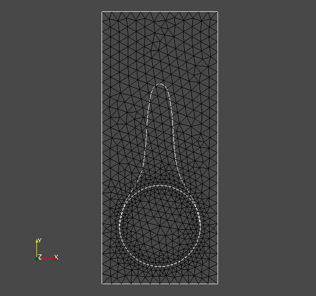
The model manifold is a sphere with radius centered in , consisting of surface nodes and edges. It is embedded in the hold-all domain , which is given by a rectangle with non-trivial boundary . The hold-all domain consists of nodes and has volume cells. They are illustrated in fig. 1. This problem is hard because solution requires a large deformation at a single local region of the initial shape. Since the mesh is locally refined near the shape, nearby cells are especially prone to degeneration by large deformations.
Notice that the manifold acts as an initial shape for the optimization routines to start. This approach is always applicable, i.e. the manifold for the pre-shape space can always be picked as the initial shape. With this, the corresponding starting pre-shape is the identity of .
For the shape optimization problem, we employ a piecewise constant source term varying dependent on the shape
| (44) |
A perimeter regularization with parameter is added as well. Combining this, the optimization problem takes the form
| (45) | ||||
To calculate the target of the shape problem, we use the source term eq. 44 and solve the Poisson problem for the target shape pictured in fig. 1. Problem eq. 45 is formulated using the classical shape space approach, since the control variable is stemming from the shape space , and represents eq. 1 from the theoretical section 2.
Next, we reformulate eq. 45 using pre-shapes, while we also add the regularizing term for shape mesh quality with parameter
| (46) | ||||
We remind the reader, that the regularizer can only be added in the pre-shape context, since it is not shape differentiable.
Technically, the combined volume and shape mesh quality regularized problem is given by formulating a bi-level problem with volume regularizing objective as the upper level problem and lower level problem eq. 46, i.e.
| (47) | ||||
We remind the reader that, despite its intimidating form, bi-level problem eq. 47 has guaranteed existence of solutions by theorem 3. The same is true for the shape regularized problem eq. 46 by theorem 1.
3.1.2 Constructing Initial and Target Node Densities and
To explicitly construct the regularizing terms, we need initial node densities of and of . Also, we need to specify target node densities and , which describe the cell volume structure of optimal meshes representing and .
The approach used in this work is to represent the initial point distributions and by using a continuous Galerkin Ansatz with linear elements similar to [12, Ch. 3]. Degrees of freedom are situated at the mesh vertices and set to the average of inverses of surrounding cell volumes, i.e.
| (48) |
In the shape case , a vertex is part of the initial discretized shape and is the set of its neighboring cells in . For -dimensional cells correspond to edges, for -dimensional to faces. In the volume mesh case , is a vertex of the initial discretized hold-all domain and is the set of its neighboring volume cells in .
Next, we specify a way to construct target parameterizations and , together with their pre-shape material derivatives. We define a target for shape parameterization tracking by a global target field . In order to satisfy normalization condition eq. 3, which is necessary for existence of solutions and stable algorithms, a normalization is included. This gives
| (49) |
With this construction, the targeted parameterization of depends on its location and shape in , as is allowed to vary on the whole domain.
The according material derivative is derived in [12] and has closed form
| (50) |
Notice that eq. 50 includes both normal and tangential components. However, only its tangential component is needed if regularized gradient systems eq. 13 and eq. 38 are applied. We will write down explicit right hand sides to gradient systems for our exemplary problem in section 3.1.3.
For a volume target , we have to satisfy the different normalization condition eq. 24 to guarantee existence of solutions. We propose to use a field defined on the hold-all domain. Then, an according target can be defined as
| (51) |
This is different to the construction of targets for embedded shapes, since the function does only change in order to guarantee normalization condition eq. 24. It cannot vary due to the change of shape of , which remains fixed. This stays in contrast to the situation for , which can change its position in . Also notice that as defined in eq. 51 can be non-continuous on the shape . However, in existence and consistency results theorem 2 and theorem 3 we have not demanded continuity or smoothness of on the entire domain . Smoothness of is only demanded for the inner and outside partitioned by .
Now we derive the pre-shape material derivative for directions . These directions are not forced to vanish on the shape , which is needed to assemble combined gradients systems with acting as test functions. This poses a difficulty in its derivation, the partitioning depends on the pre-shape , but not on . Let us fix a and compute on the outer domain with pre-shape calculus rules from [12]. In this computation we write instead of for readability.
| (52) | ||||
Here, is the outer unit normal vector field on , and is the outer unit normal vector field on . In particular, we used that and do neither depend on nor on , which lets their pre-shape derivatives vanish. Also, we have applied Gauss’ theorem and used . Notice the change of sign for the first summand of the last equality, due to on . Analogous computation on the interior with boundary give us the pre-shape material derivative
| (53) |
This pre-shape material derivative is interesting from a theoretical perspective, since it is an example of a derivative depending on the shape of a submanifold , where the actual pre-shape at hand is of different dimension. Also, we see that the sign of boundary integral on depends on whether the inside or outside of is regarded. This nicely reflects that changing adds volume on one side and takes it away from the other. We remind the reader that normal directions are not normal directions corresponding to the shape of . They rather lie in the interior of , and hence are part of the fiber or tangential component of .
3.1.3 Pre-Shape Gradient Systems
To compute pre-shape gradients we need suitable bilinear forms . The systems for our gradients are always of form
| (54) | ||||
In our numerical implementations, we test two bilinear forms and four different right hand sides. We abbreviate the right hand sides by depending on pre-shapes and test functions , and boundary conditions by . First, we consider the weak formulation of the linear elasticity equation with zero first Lamé parameter as found in [17]
| (55) | ||||
As the second bilinear form, we consider the weak formulation of the vector valued -Laplacian equation. Since systems stemming from the -Laplacian have the issue to be indefinite, we employ a standard regularization by adding a parameter . To make a comparison with the linear elasticity eq. 55 viable, we use a local weighting in the bilinear form, which then is
| (56) |
We chose the local weighting as the solution of Poisson problem
| (57) |
for . In the context of linear elasticity eq. 55 it can be interpreted as the so-called second Lamé parameter.
Remark 10 (Sufficiency of Linear Elements for Pre-Shape Regularization).
In order to apply pre-shape regularization approaches presented in this work, it is completely sufficient to use continuous linear elements to represent involved functions. As we can see in the pre-shape derivative formulas eq. 8 and eq. 30, the highest order of featured derivatives is one. This is important for application in practice, since existing shape gradient systems do not require higher order elements for volume and shape mesh quality tracking. In particular, all following systems are built by using continuous first order elements in FEniCS.
Next, we need the shape derivative of the PDE constrained tracking type shape optimization objective . It can be derived by a Lagrangian approach using standard shape or pre-shape calculus rules, giving
| (58) | ||||
Here, is the adjoint solving the adjoint system
| (59) | ||||
It is straight forward to derive the shape derivative of the perimeter regularization , which takes the form
| (60) |
where is the tangential divergence of on .
In the following we give four right hand sides representing various (un-)regularized approaches to calculate pre-shape gradients. They correspond to the unregularized shape gradient, the shape parameterization tracking regularized pre-shape gradient, the volume and parameterization tracking regularized pre-shape gradient, and the volume and parameterization tracking regularized pre-shape gradient with free tangential outer boundary.
For the unregularized shape gradient, the right hand side of the gradient system eq. 54 takes the standard form
| (61) | ||||
In this case, the respective boundary condition for the gradient system is simply a Dirichlet zero condition .
Next, we give the right hand side for the shape parameterization regularized pre-shape gradient. For shape parameterization tracking, we employ a target given by a globally defined function (cf. eq. 49), which in combination yields
| (62) | ||||
The boundary condition is Dirichlet zero . In order to assemble the shape regularization , it is necessary to compute the tangential Jacobian . In applications, this means storing the vertex coordinates becomes of the initial shape is necessary. Then can be calculated simply as the difference of current shape node coordinates to the initial ones. Hence there is no need to invert matrices to calculate . We give a strong reminder that is the covariant derivative, and must not be confused with the tangential derivative (cf. [12, Ex. 2]). In the case of an -dimensional manifold , the covariant derivative is a -matrix, whereas the tangential derivative is . The use of covariant derivatives requires to calculate local orthonormal frames, which can be done by standard Gram-Schmidt algorithms. Knowing this, the computation of Jacobian determinants is inexpensive, since matrices from applications are of size smaller .
Building on eq. 62, we can construct the right hand side for the shape and volume parameterization regularized pre-shape gradient. For this, we use a volume tracking target defined by a field (eq. 51). This finally gives
| (63) | ||||
The last two integrals correspond to the regularizer for volume parameterization tracking. As in previous cases, the corresponding Dirichlet condition is given by . All previous remarks on assembling the right and side are still valid. Additionally, it is necessary to store coordinates of the entire initial hold-all domain. With these, the volume pre-shape can be calculated as the difference of initial to current coordinates the volume mesh. For volume regularization, calculation of Jacobian determinants does not require local orthonormal frames via Gram-Schmidt algorithms, as no covariant derivatives are used. It is very important to use a correct normalization for to ensure existence of solutions. This is necessary, since in practical applications an optimization step leads to change of the underlying shape, and thus inner and outer components of . Hence it is not enough to simply estimate once in the beginning. Either, needs to be estimated by eq. 48 in every iteration in which the shape of changes. Or is replaced by , which is motivated by the transformation rule. We have decided for the latter, which can be seen in the last two terms of eq. 63. This also needs to be taken into account when calculating , e.g. for line search. As explained in section 2.2.3, it is necessary to use as directions for the volume regularization, if shapes are enforced to stay invariant. The projection can be realized by setting the degrees of freedom of the finite element representation of to zero on the shape . This leads to vanishing of the first term of (cf. eq. 53), which does not occur in eq. 63.
Lastly, the right hand side for a volume and parameterization tracking regularized pre-shape gradient with free tangential outer boundary is given by eq. 63 as well. However, instead of employing Dirichlet zero boundary conditions, we permit the boundary to move tangentially. For this, we set
| (64) |
for a scaling factor . Here, is the -representation of tangential components of , i.e
| (65) |
Notice that in practice, this does not require solution of a PDE on , since the tangential values of can be extracted directly from its finite element representation. We remind the reader that this is more a heuristic approach, which we will refine in further works.
3.2 Numerical Results and Comparison of Algorithms
In this subsection we explore computational results of employing unregularized and various pre-shape regularized gradient descents for shape optimization problem eq. 45. We propose an algorithm 1, which is a modified gradient descent method with a backtracking line search featuring regularized gradients. We present 7 implementations of pre-shape gradient descent methods. The first 4 feature the linear elasticity metric eq. 55 with unregularized, shape regularized, volume and shape regularized, and volume and shape regularized free tangential outer boundary right hand sides. The other 3 feature the regularized -Laplacian metric eq. 56 with unregularized, shape regularized, volume and shape regularized right hand sides. For the -Laplacian metric we dismiss the free tangential outer boundary regularization, since solving it requires a modified Newton’s method and slightly complicates our approach. Both the linear elasticity metric eq. 55 and the regularized -Laplacian metric eq. 56 involve a local weighting function stemming from eq. 57 inspired by [17]. The two approaches for these metrics without any type of pre-shape regularization are denoted as their ’Vanilla’ versions. For implementations we use the open-source finite-element software FEniCS (cf. [11, 1]). Construction of meshes is done via the free meshing software Gmsh (cf. [7]). We perform our calculations using a single Intel(R) Core(TM) i5-3210M CPU @ 2.50GHz featuring 6 GB of RAM.
Algorithm 1 is essentially a steepest descent with a backtracking line search. The regularization procedures for shape and volume mesh quality take place by modifying the right hand sides as described in section 3.1.3. However we want to pinpoint some important differences of algorithm 1 compared to a standard gradient descent for shape optimization. First, notice that the initial mesh coordinates are stored in order to calculate and . This corresponds to setting initial pre-shapes and . Since the current mesh coordinates are necessarily stored in a standard gradient descent, and are calculated as mesh coordinate differences. Calculating these inverse embeddings amounts to a matrix difference operation, and therefore is of negligible computational burden. Estimating initial vertex distributions and needs to be done only once at the beginning of our routine. Hence it does not contribute to computational cost in a significant way. If shape regularization is partaking in the gradient system, it is necessary to compute and store local tangential orthonormal frames of the initial shape . Together with calculation of local tangential orthonormal frames for the current shape , these are used to assemble the covariant Jacobian determinant for the regularized right-hand side of the gradient systems. Since this need to be done for each new iterate , it indeed increases computational cost. If required, this can be mitigated by parallel computing, since tangential orthonormal bases can be calculated simultaneously for all points . Another difference to standard steepest descent methods concerns the condition of convergence in line of algorithm 1. It features two conditions, namely sufficient decrease in either the absolute or relative norm of the pre-shape gradient, and sufficient decrease of relative values for the original shape objetive . We use this approach, since several objective functionals participate simultaneously in formation of pre-shape gradients . If shape or volume regularization take place, they influence the size of gradients depending on the mesh quality. In order to compare different (un-)regularized gradient systems, we use this criterion to guarantee the same decrease of the original problem’s objective for all strategies. For the same reason, the line search checks for a sufficient decrease of the combined objective functionals matching the gradient regularizations. In some sense, this is a weighted descent for multi criterial optimization, where the objectives are and regularizations and .
Furthermore, we mention the difference of our two tested metrics acting as left hand sides. The linear elasticity metric eq. 55 leads to a linear system, which is solvable by use of standard techniques such the CG-method. It is reported in [13], that the -Laplacian metric has particular advantages in resolution of sharp edges or kinks of optimal shapes. Illustration of this is not the goal of this paper. However, the -Laplacian system eq. 56 is increasingly non-linear for larger . This significantly increases computational cost and burden of implementation, since Newton’s method requires multiple linear system solves. Also, systems are possibly indefinite if regularization parameter is too small. If chosen too large, we pay for positive definiteness by overregularizing the gradient systems. In order to achieve convergence of Newton’s method for the -Laplacian, we use gradients from the previous shape optimization step as an initial guess.
Remark 11 (Integrating Shape and Volume Regularization in Existing Solvers).
Implementing shape and volume regularization with the pre-shape approach does not require a big overhead, if an existing solver for the shape optimization problem of concern is available. It solely requires accessibility of gradient systems eq. 54 and mesh morphing to update meshes and shapes. With this, adding regularization terms in style of eq. 62 or eq. 63 to existing right hand sides is all that needs to be done. This does not affect the user’s choice of preferred metrics to represent gradients. We highlight this by implementing and comparing our regularizations for the linear elasticity and the non-linear -Laplacian metrics. From this perspective, algorithm 1 is only an in-depth explanation how right-hand side modifications of gradient systems are assembled.
For a meaningful comparison of the mentioned approaches, we use the same parameters for the problem throughout. Parameters for source term of the PDE constraint in eq. 59 are chosen as and . The scaling factor for perimeter regularization is . Parameters for calculating local weightings via eq. 57 are and for all approaches. The stopping criteria for all routines tested remain the same. Specifically, the tolerance for relative decrease of gradient norms is , absolute decrease of gradient norms and relative main objective decrease . If shape regularization is employed, it is weighted with and uses a constant target . This targets a uniform distribution of surface cell volume of shapes. For volume regularization, the weighting is with a constant targeting uniform volume cells of the hold-all domain. If we permit free tangential movement of the outer boundary eq. 64, we choose a weighting parameter . In case of the -Laplacian metric, we chose a parameter . Its regularization parameter is chosen as for the unregularized, and shape and volume regularized routines. If shape without volume regularization takes place, we had to increase regularization to . This was necessary, since at some point lower values for resulted in indefinite systems during descent with -Laplacian gradients.
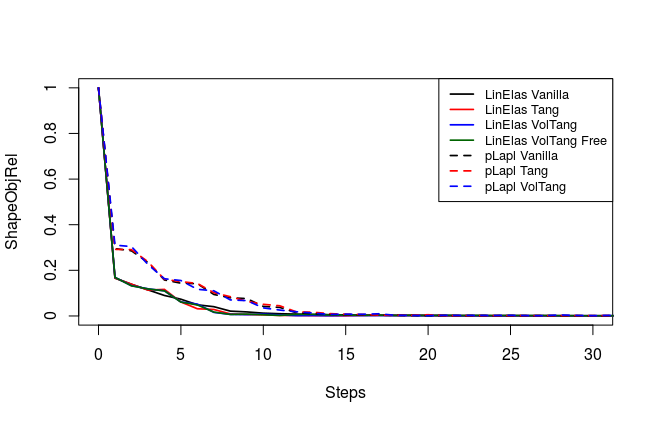
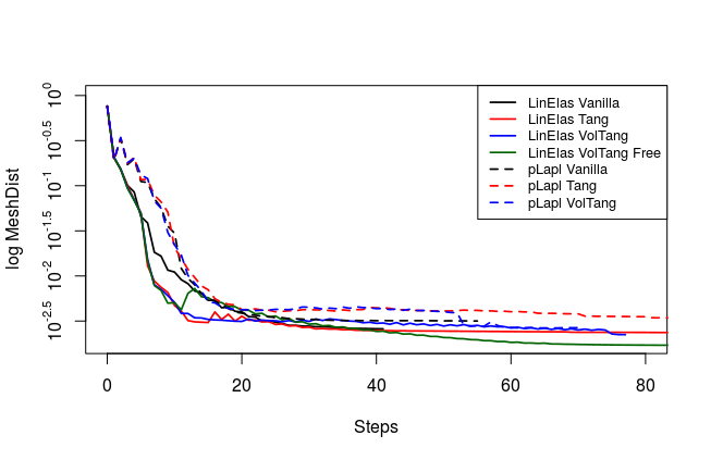
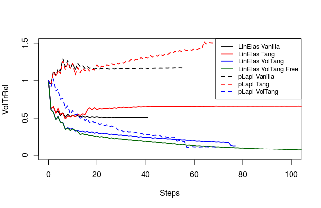
We compare relative values of , and , which are illustrated in fig. 2. Here, is interpretable as the deviation of the shape mesh from a surface mesh with equidistant edges. Similarly, can be understood as the deviation of the volume mesh from a volume mesh with uniform cell volumes. Since a change of mesh coordinates leads to different qualities of solutions to the PDE constraint of eq. 45, the regularizations do affect the original objective . Hence, we also measure distance of shapes and the target shape by a Hadamard like distance function
| (66) |
This gives us a geometric value for convergence of our algorithms, complementing the value of objective functionals for our results.
| LE Vanilla | LE Tang | LE VolTang | LE VolTang Free | -L Vanilla | -L Tang | -L VolTang | |
| total time | 49.0s | 345.4s | 199.9s | 320.7s | 135.4s | 316.5s | 325.8s |
| avg. time step | 1.2s | 2.5s | 2.6s | 2.8s | 2.4s | 2.0s | 4.6s |
| number steps | 41 | 137 | 77 | 114 | 55 | 155 | 70 |
From fig. 2 and , we see that all methods are converging. They all minimize the original shape objective , and the geometric mesh distance to the target shape (cf. fig. 1). Seeing that mesh distance is minimized for all methods confirms that the optimal shape of original problem eq. 45 is left invariant by our pre-shape regularizations. Also, convergence to the optimal shape is not affected by the choice of regularization and metric . In fig. 2 we also see that, given a fixed metric , the values of original target for regularized routines vary only slightly from the unregularized one. This means that intermediate shapes are left nearly invariant by all regularization approaches as well. We witness that the -Laplacian metric eq. 56 gives a pre-shape gradient with slightly slower convergence if compared to the linear elasticity eq. 55 for unregularized and all regularized variants. However, one should keep in mind that the shapes considered here have rather smooth boundary. Notice that all gradients are normed in the line search of algorithm 1, which permits this comparison.
In table 1 we present the times for all optimization runs. We see that the fastest method in both time and step count featured the unregularized approach with the linear elasticity metric. Regularized approaches all need more steps for convergence, since the convergence condition features sufficient minimization of the gradient norms. As shape and volume tracking objectives and participate in this condition, the optimization routine continues to optimize for mesh quality, despite a sufficient reduction of the original target . This can be verified in fig. 2. Notice that additional volume regularization did not considerably increase average computational time per step for the linear elasticity approach. The times for approaches featuring shape regularization can be improved by computing tangential orthonormal bases in parallel. We relied on a rather inefficient but convenient calculation of these solving several projection problems using FEniCS.
From table 1, we see that the unregularized -Laplacian approach for needs more steps to convergence compared to a linear elasticity gradient. Average time per step is higher too, since Newton’s method needs to be applied to solve the non-linear gradient system. This approach needs careful selection of regularization parameter for eq. 56, since the mesh quality degrades quickly for our problem. This makes calculation of gradients by Newton’s method difficult, since conditioning of systems and indefiniteness at some point of the shape optimization routine are an issue. If the shape regularized -Laplacian gradient is compared to the unregularized -Laplacian gradient, the computational times were slightly faster on average. We amount this to faster convergence of the Newton method, since we needed to employ a higher regularization parameter for the shape regularized routine. This also explains longer computational times for the volume regularized -Laplacian, since the same regularization parameter as in the unregularized approach is permissible, but more Newton iterations are necessary. Since the shape regularization takes place simultaneously with volume regularization, a lower permissible regularization indeed shows that volume regularization improves condition of linear systems.
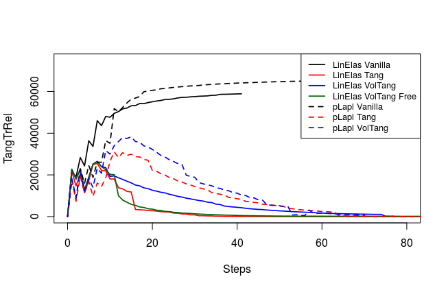
To analyze quality of the shape mesh for all routines, we provide the relative value of the shape parameterization tracking target in table 1 , as well as for final shapes in fig. 4 and fig. 7. The relative value of the shape parameterization tracking target in table 1 measures deviation of the current shape mesh from a uniform surface mesh. This means larger values indicate more non-uniformity of shape meshes. The colors in fig. 4 and fig. 7 highlight variation of node densities on the shape meshes, where a uniform color indicates approximately equidistant surface nodes. As the starting mesh seen in fig. 1 is constructed via Gmsh, it features an approximately uniform surface mesh. However, both for unregularized linear elasticity and -Laplacian approaches, we see in fig. 2 that increases during optimization. This means surface mesh quality deteriorates if no regularization takes place. For final shapes, this is visualized in fig. 4 and fig. 7 . There we clearly see an expansion of cell volumes for the targeted bump at the top. All other routines involve a shape quality regularization by . In table 1 it is visible that also for these routines, the deviation from uniform surface meshes increases initially. Once surface mesh quality becomes sufficiently bad, the shape parameterization takes effect and corrects quality until approximate uniformity is achieved. We can clearly see this by convergence of for all shape regularized methods in table 1 . Also, we see an approximately uniform color of for final shapes in fig. 4 and fig. 7, which indicates a nearly equidistant surface mesh. As a caveat, we see in fig. 3 and fig. 6 that shape without volume regularization decreases quality of the surrounding volume mesh. This happens, since surface vertices are transported from areas with low volume at the bottom to areas with high volume at the top. In case no volume regularization takes place, node coordinates from the hold-all domain are not corrected for this change. Nevertheless, if a remeshing strategy is employed for shape optimization including shape regularization, the improved surface mesh quality leads to a superior remeshed domain. Such routines are an interesting subject for further works.
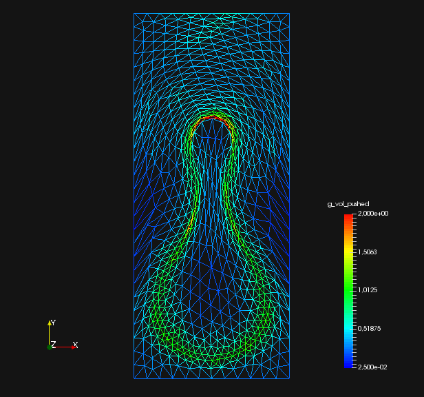
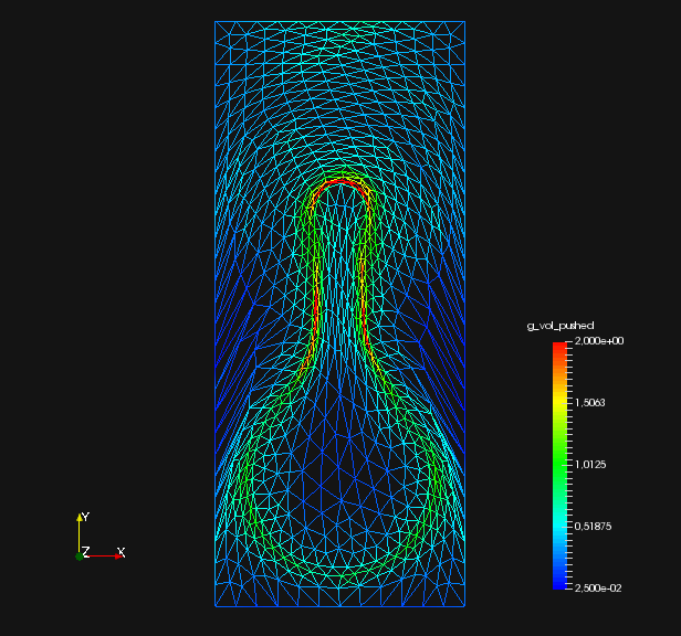
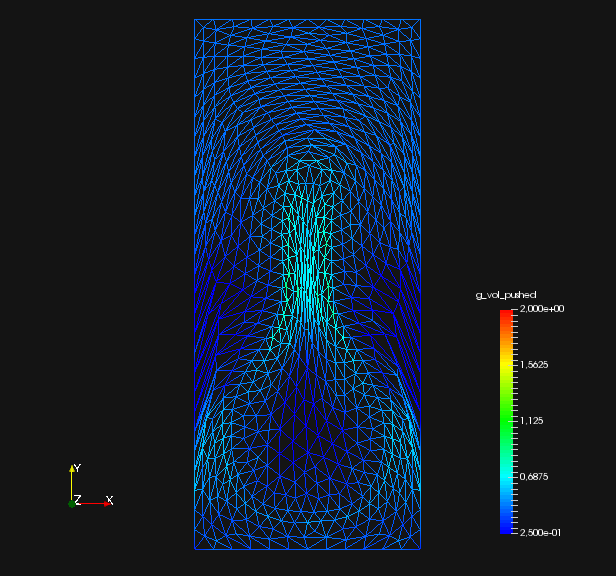
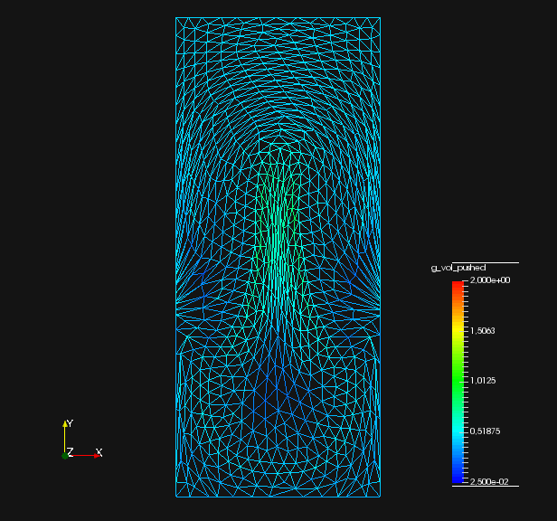
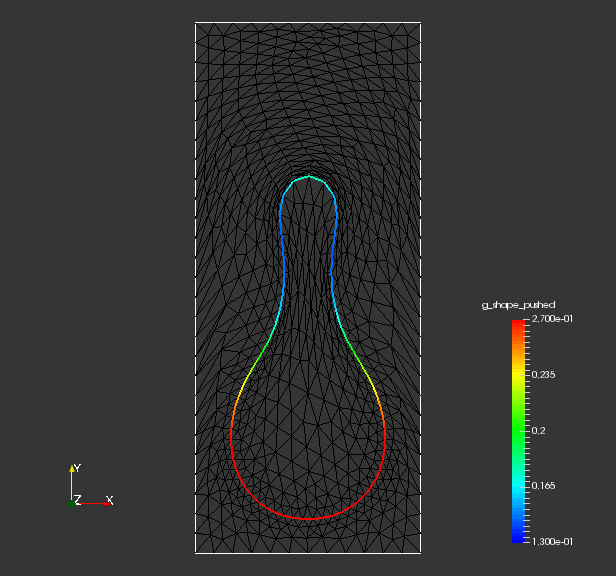
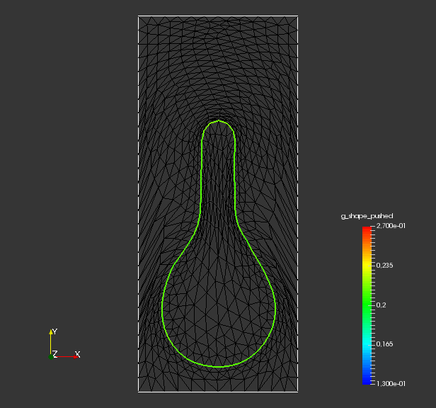
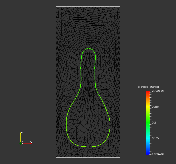
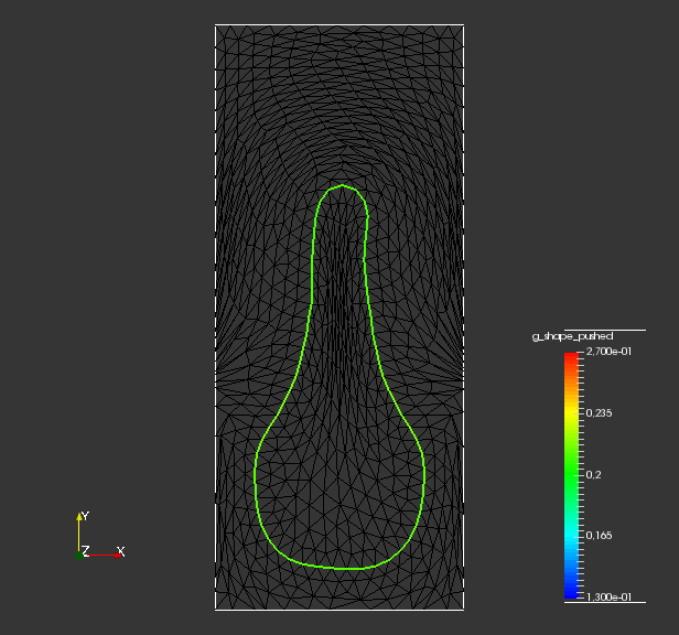
In fig. 2 relative values of the volume parameterization tracking functional are depicted for each routine and step. We interpret these values as a measure for non-uniformity of the volume mesh . The local density of volume vertices are visualizing this, and are depicted fig. 3 and fig. 6. For pictures zoomed at the upper tip of final shapes, we refer the reader to fig. 5 and fig. 8. From fig. 2 we see that, both for linear elasticity and -Laplacian metrics, non-volume regularized approaches have significantly higher value of . Values even increase for the -Laplacian metric, while there is a slight decrease for the linear elasticity. Notice that the initial mesh is locally refined near the shape , which naturally increases the initial value of for a uniform target. As already discussed, we see in fig. 2 that shape regularized approaches reduce quality of the volume mesh even further compared to unregularized approaches. The decrease of mesh quality especially visible in zoomed pictures fig. 5 and fig. 8 and . We see that for these approaches, volume cells near the shape are compressed to such an extent that their volumes nearly vanish. Also, the cell volume distribution for unregularized and shape regularized approaches varies dramatically, which can be seen in fig. 3 and fig. 6 and . If volume regularization is applied, we see in fig. 2 that convergence for takes place independent of the metric being used. This is apparent when looking at the volume mesh quality in fig. 3 and and fig. 6 . Further notice that in fig. 5 and and fig. 8 severe compression of cells neighboring the top of final shapes is avoided. Volume cells inside the neck of final shapes are still more or less compressed for all approaches. The interior cell volume cannot be transported through the shape, since it is forced to stay invariant. Since the mesh topology is not changed during the optimization routine, there is also limited possibility to redistribute the cell volumes inside the shape. This situation could be remedied by cell fusion, edge swapping or remeshing strategies, which is beyond the scope of this article. Finally, we want to highlight the difference of volume regularizations with and without free tangential outer boundary . If fig. 3 and are compared, we see that the nodes on the outer boundary changed position for routine . Indeed, the cell volume distribution is more uniform for free outer boundary routine , which is visualized by less variation of color. This leads to even further increase of volume mesh quality, which can be pinpointed in fig. 2 .
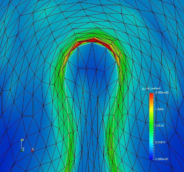
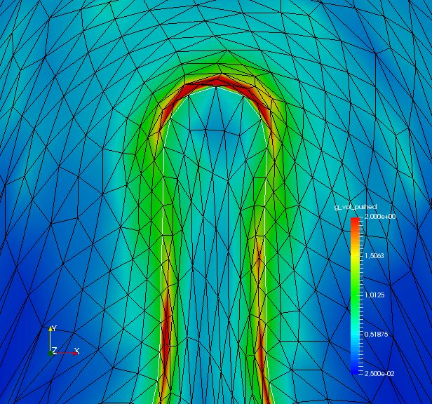
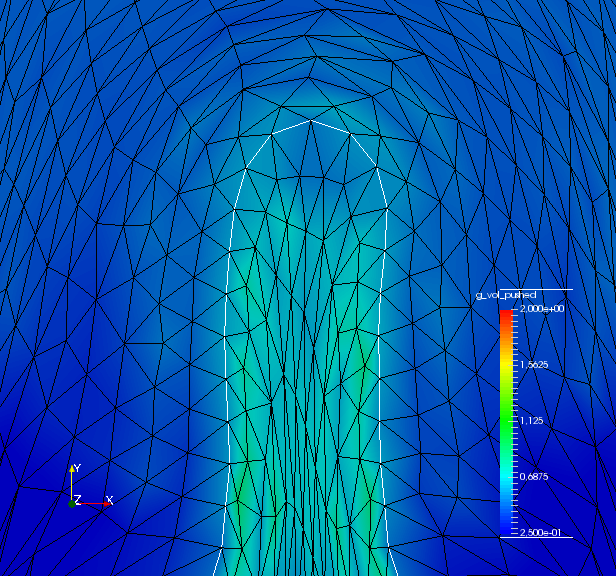
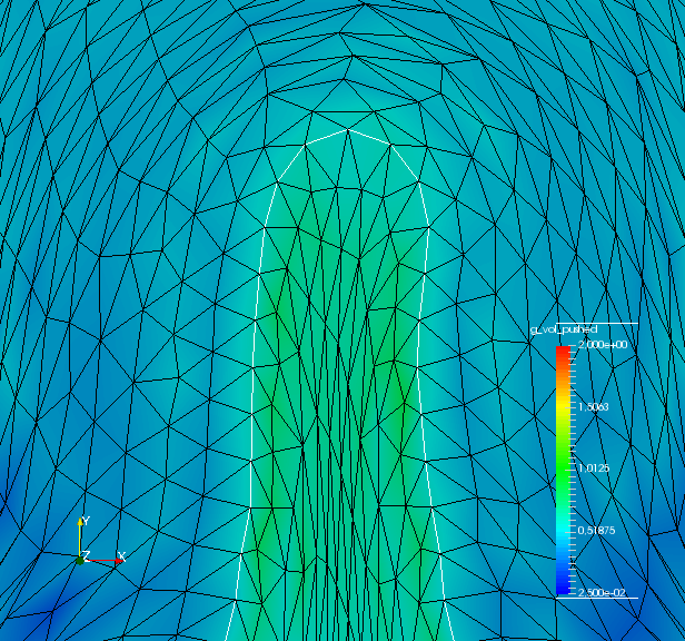
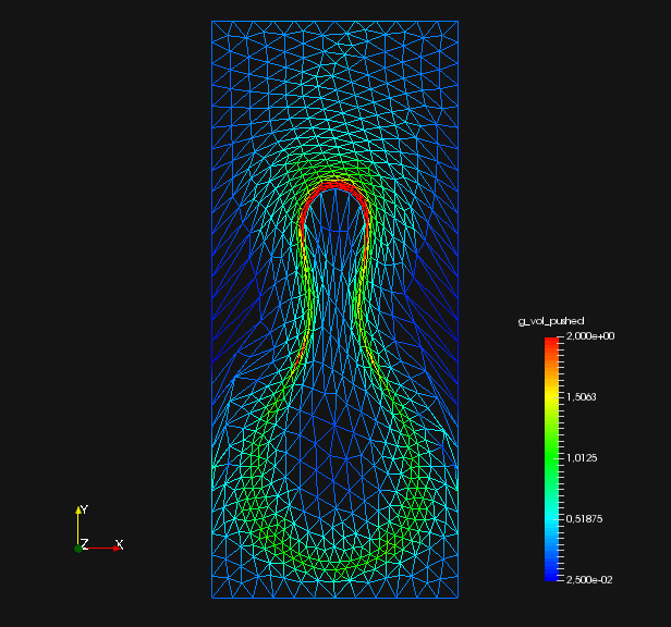
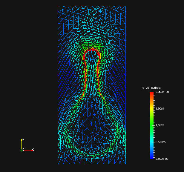
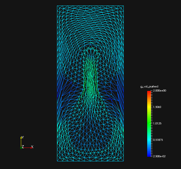
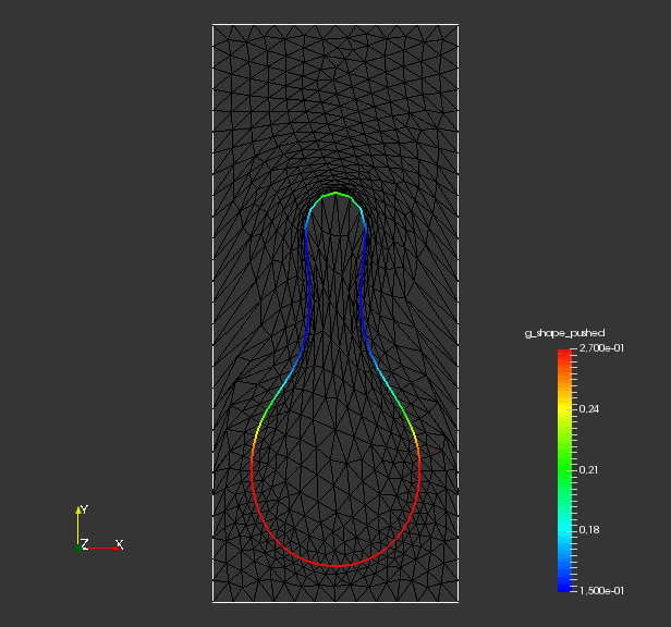
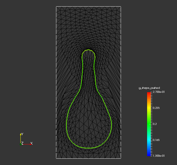
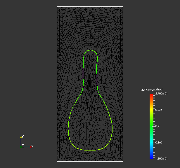
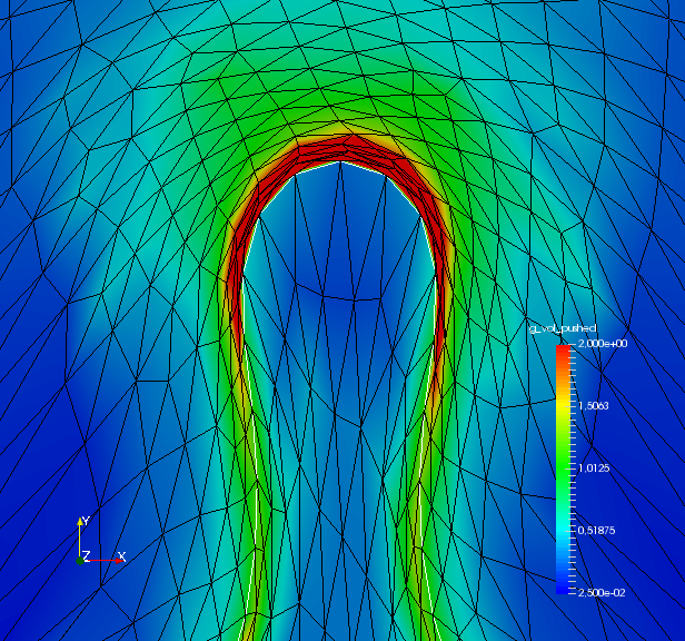
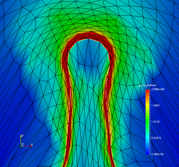
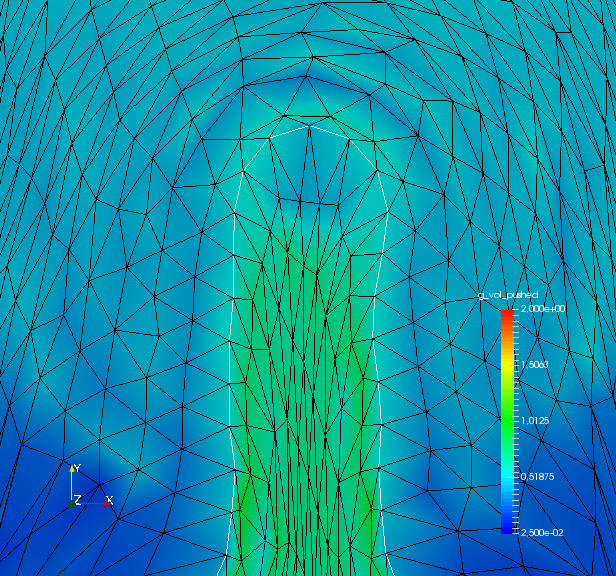
4 Conclusion and Outlook
In this work, we have provided several approaches to regularize general shape optimization problems to increase shape and volume mesh quality using pre-shape calculus. Existence of regularized solutions and consistency of modified pre-shape gradient systems is guaranteed by several results for simultaneous shape and volume tracking. With the presented gradient system modifications, our goal of leaving optimal shapes to the original problem invariant was achieved. The computational burden is limited, since no additional solution of linear systems for regularized pre-shape gradients is necessary. We also successfully implemented and compared our pre-shape gradient regularization approaches for linear elasticity and non-linear -Laplacian metrics.
There are several possibilities to further develop pre-shape regularization approaches. For one, non-constant targets can be designed to adapt mesh refinement non-uniformly. In particular, mesh quality targets increasing solution quality of PDE constraints can be envisioned. Also, we did not touch the topic of pre-shape Hessian, which could be of use to further increase effectiveness of regularization approaches. Furthermore, a combination with discrete techniques, such as remeshing and edge swapping are possible as well.
Acknowledgements
The authors would like to thank Michael Hinze (Koblenz University) and Martin Siebenborn (Universität Hamburg) for a helpful and interesting discussion on the -Laplacian metric. This work has been supported by the BMBF (Bundesministerium für Bildung und Forschung) within the collaborative project GIVEN (FKZ: 05M18UTA). Further, the authors acknowledge the support of the DFG research training group 2126 on algorithmic optimization.
References
- [1] M.S. Alnæs, J. Blechta, J. Hake, A. Johansson, B. Kehlet, A. Logg, C. Richardson, J. Ring, M.E. Rognes, and G.N. Wells. The FEniCS project version 1.5. Archive of Numerical Software, 3(100), 2015.
- [2] W. Cao, W. Huang, and R.D. Russell. A Study of Monitor Functions for Two-Dimensional Adaptive Mesh Generation. SIAM Journal on Scientific Computing, 20(6):1978–1994, 1999.
- [3] B. Dacorogna and J. Moser. On a Partial Differential Equation Involving the Jacobian Determinant. In Annales de l’Institut Henri Poincare (C) Non Linear Analysis, volume 7, pages 1–26. Elsevier, 1990.
- [4] K. Deckelnick, P.J. Herbert, and M. Hinze. A Novel Approach to Shape Optimisation with Lipschitz Domains. arXiv preprint arXiv:2103.13857, 2021.
- [5] T. Etling, R. Herzog, E. Loayza, and G. Wachsmuth. First and second order shape optimization based on restricted mesh deformations. arXiv preprint arXiv:1810.10313, 2018.
- [6] J. Friederich, G. Leugering, and P. Steinmann. Adaptive Finite Elements based on Sensitivities for Topological Mesh Changes. Control and Cybernetics, 43, 2014.
- [7] C. Geuzaine and J.-F. Remacle. Gmsh: A Three-Dimensional Finite Element Mesh Generator with Built-In Pre-and Post-Processing Facilities. In Proceedings of the Second Workshop on Grid Generation for Numerical Computations, Tetrahedron II, 2007.
- [8] V. Guillemin and A. Pollack. Differential Topology, volume 370. American Mathematical Soc., 2010.
- [9] J. Haubner, M. Siebenborn, and M. Ulbrich. A Continuous Perspective on Modeling of Shape Optimal Design Problems. arXiv preprint arXiv:2004.06942, 2020.
- [10] R. Herzog and E. Loayza-Romero. A Manifold of Planar Triangular Meshes with Complete Riemannian Metric. arXiv preprint arXiv:2012.05624, 2020.
- [11] A. Logg, K.-A. Mardal, G.N. Wells, et al. Automated Solution of Differential Equations by the Finite Element Method. Springer, 2012.
- [12] D. Luft and V. Schulz. Pre-Shape Calculus: Foundations and Application to Mesh Quality Optimization. arXiv preprint arXiv:2012.09124, 2020.
- [13] P.M. Müller, N. Kühl, M. Siebenborn, K. Deckelnick, M. Hinze, and T. Rung. A novel p-Harmonic Descent Approach applied to Fluid Dynamic Shape Optimization. ArXiv, 2021.
- [14] S. Onyshkevych and M. Siebenborn. Mesh Quality Preserving Shape Optimization using Nonlinear Extension Operators. arXiv preprint arXiv:2006.04420, 2020.
- [15] G. Savard and J. Gauvin. The Steepest Descent Direction for the Nonlinear Bilevel Programming Problem. Operations Research Letters, 15(5):265–272, 1994.
- [16] S. Schmidt. A Two Stage CVT/Eikonal Convection Mesh Deformation Approach for Large Nodal Deformations. arXiv preprint arXiv:1411.7663, 2014.
- [17] V. H. Schulz and M. Siebenborn. Computational Comparison of Surface Metrics for PDE Constrained Shape Optimization. Computational Methods in Applied Mathematics, 16(3):485–496, 2016.
- [18] V.H. Schulz, M. Siebenborn, and K. Welker. Efficient PDE Constrained Shape Optimization based on Steklov-Poincaré Type Metrics. SIAM Journal on Optimization, 26(4):2800–2819, 2016.
- [19] J.R. Shewchuk. What is a Good Linear Element? Interpolation, Conditioning, Anisotropy, and Quality Measures. Univ. of California, Berkeley, CA, 2002.
- [20] N.K. Smolentsev. Diffeomorphism groups of compact manifolds. Journal of Mathematical Sciences, 146(6):6213–6312, 2007.