Simultaneous Reduction of Number of Spots and Energy Layers in Intensity Modulated Proton Therapy for Rapid Spot Scanning Delivery

We discretize the patient’s body into $m$ voxels and the proton beams into $n$ spots. For each spot $j\in\{1,\ldots,n\}$, we calculate the radiation dose delivered by a unit intensity of that spot to voxel $i\in\{1,\ldots,m\}$ and call this value $A_{ij}$. The dose influence matrix is then $A\in\mathbf{R}_{+}^{m\times n}$, where its rows correspond to the voxels and its columns to the spots. Let $p\in\mathbf{R}_{+}^{m}$ be the prescription vector, i.e., $p_{i}$ equals the physician-prescribed dose if $i$ is a target voxel and zero otherwise. We concatenate the spot intensities of all beams and all energy layers within each beam, denoting this collective as the vector $x\in\mathbf{R}^{n}$. The typical treatment planning problem seeks a vector of spot intensities $x$ that minimizes the deviation of the delivered dose, $d=Ax$, from the prescription $p$. This deviation can be decomposed into a penalty on the overdose, $\overline{d}=(d-p)_{+}=\max(d-p,0)$, and the underdose, $\underline{d}=(d-p)_{-}=-\min(d-p,0)$, which we combine to form the cost function

$$f(\overline{d},\underline{d})=\sum_{i=1}^{m}\overline{w}_{i}\overline{d}_{i}^{2}+\underline{w}_{i}\underline{d}_{i}^{2},$$

(1)

where $\overline{w},\underline{w}\in\mathbf{R}_{+}^{n}$ are penalty parameters that determine the relative importance of the over/underdose to the treatment plan. (Note the underdose is ignored for non-target voxels $i$ because $p_{i}=0$).

Dose constraints are defined for each anatomical structure. For a given structure $s$, let $A^{s}\in\mathbf{R}_{+}^{m_{s}\times n}$ be the row slice of $A$ containing only the rows of the $m_{s}$ voxels in $s$. A maximum dose constraint takes the form of $A^{s}x\leq d_{s}^{\textrm{\tiny max}}$, where $d_{s}^{\textrm{\tiny max}}$ is an upper bound. Similarly, a mean dose constraint is of the form $\frac{1}{m_{s}}\mathbf{1}^{T}A^{s}x\leq d_{s}^{\textrm{\tiny mean}}$. By stacking the constraint matrices/vectors for all $S$ structures, we can represent the set of dose constraints as a single linear inequality $Bx\leq c$, where $B=[A^{1},\frac{1}{m_{1}}\mathbf{1}^{T}A^{1},\ldots,A^{S},\frac{1}{m_{S}}\mathbf{1}^{T}A^{S}]$ and $c=[d_{1}^{\textrm{\tiny max}},d_{1}^{\textrm{\tiny mean}},\ldots,d_{S}^{\textrm{\tiny max}},d_{S}^{\textrm{\tiny mean}}]$. Then, our treatment planning problem is

$$\begin{array}[]{ll}\mbox{minimize}&f(\overline{d},\underline{d})\\ \mbox{subject to}&\overline{d}=(Ax-p)_{+},\quad\underline{d}=(Ax-p)_{-},\quad Bx\leq c\\ &x\geq 0,\quad\overline{d}\geq 0,\quad\underline{d}\geq 0\end{array}$$

(2)

with variables $x\in\mathbf{R}^{n},\overline{d}\in\mathbf{R}^{m}$, and $\underline{d}\in\mathbf{R}^{m}$. Since the objective function $f$ is monotonically increasing in $\overline{d}$ and $\underline{d}$ over the nonnegative reals, we can write this problem equivalently as

$$\begin{array}[]{ll}\mbox{minimize}&f(\overline{d},\underline{d})\\ \mbox{subject to}&Ax-\overline{d}+\underline{d}=p,\quad Bx\leq c\\ &x\geq 0,\quad\overline{d}\geq 0,\quad\underline{d}\geq 0.\end{array}$$

(3)

(The derivation is provided in appendix A). Problem 3 is a convex quadratic program (QP), hence can be solved using standard convex methods, e.g., the alternating direction method of multipliers (ADMM) [BPC⁺11, FTZ23] or interior-point methods [Wri97, Gor22]. The reader is referred to S. Boyd and L. Vandenberghe (2004) [BV04] and J. Nocedal and S. J. Wright (2006) [NW06] for a thorough discussion of convex optimization.

The cost function defined in 1 focuses solely on the difference of the delivered dose from the prescription, i.e., the dosimetric plan quality. However, in our treatment scenario, we are also interested in reducing the dose delivery time, i.e., increasing the plan delivery efficiency. The delivery time is positively correlated with the number of nonzero spots (spot scanning rate) and nonzero energy layers (energy switching time) [GCM⁺20, PEL⁺18]. Thus, we want to augment the objective of problem 3 with a regularization function $r:\mathbf{R}^{n}\rightarrow\mathbf{R}$, which penalizes the spot vector $x$ in a way that reduces the number of nonzero spots/layers, while maintaining high plan quality. The regularized treatment planning problem is

$$\begin{array}[]{ll}\mbox{minimize}&f(\overline{d},\underline{d})+\lambda r(x)\\ \mbox{subject to}&Ax-\overline{d}+\underline{d}=p,\quad Bx\leq c\\ &x\geq 0,\quad\overline{d}\geq 0,\quad\underline{d}\geq 0\end{array}$$

(4)

with respect to $x,\overline{d}$, and $\underline{d}$. Here we have introduced a regularization weight $\lambda\geq 0$ to balance the trade-off between dosimetric plan quality, represented by the cost $f(\overline{d},\underline{d})$, and plan delivery efficiency, as captured by the regularization term $r(x)$. A larger value of $\lambda$ places more importance on efficiency.

In the following subsections, we review a few regularization functions that have been suggested in the literature. Let $\mathcal{J}=\{1,\ldots,n\}$ and $\mathcal{G}=\{\mathcal{J}_{1},\ldots,\mathcal{J}_{G}\}$ be a set of subsets of $\mathcal{J}$, where each $\mathcal{J}_{g}\subseteq\mathcal{J}$ has exactly $n_{g}\leq n$ elements. Specifically in our setting, $\mathcal{G}$ represents a partition of $n$ spots into $G$ energy layers with $\mathcal{J}_{g}$ containing the indices of the $n_{g}$ spots in layer $g$.

As we have discussed, the $l_{1}$ regularization function promotes sparsity of the spots, but not the energy layers. The group $l_{2}$ regularization function promotes sparsity of the layers, but not the spots – indeed, it tends to produce dense spot vectors due to the $l_{2}$ norm. In this section, we introduce the reweighted $l_{1}$ regularization method, which promotes sparsity in both the spots and the energy layers.

The reweighted $l_{1}$ method assigns a weight to every spot based on its intensity and energy layer. The weights are chosen to counteract the intensity of each layer, so that all spots, regardless of intensity, contribute roughly equally to the total regularization penalty. This is done to imitate the “ideal” group $l_{0}$ regularizer (equation 6), which counts every nonzero layer as one unit (due to $\mathbf{card}$) regardless of intensity.

Formally, we define the weighted group $l_{1}$ regularizer

$$r_{3}(x;\beta)=\sum_{g=1}^{G}\beta_{g}\sum_{j\in\mathcal{J}_{g}}|x_{j}|$$

(9)

with weight parameters $\beta_{g}\in\mathbf{R}_{+}\cup\{+\infty\}$ for $g=1,\ldots,G$. An intuitive way to set $\beta_{g}$ is to make it inversely proportional to the optimal total intensity of energy layer $g$, i.e.,

$$\beta_{g}=\begin{cases}\frac{1}{\sum_{j\in\mathcal{J}_{g}}x_{j}^{\star}}&\sum_{j\in\mathcal{J}_{g}}x_{j}^{\star}\neq 0\\ +\infty&\sum_{j\in\mathcal{J}_{g}}x_{j}^{\star}=0\end{cases},$$

where $x^{\star}\in\mathbf{R}_{+}^{n}$ is an optimal spot vector. However, we do not know $x^{\star}$ beforehand. We will approximate this weighting scheme iteratively using the reweighted $l_{1}$ method.

The reweighted $l_{1}$ method is a type of majorization-minimization (MM) algorithm, which solves an optimization problem by iteratively minimizing a surrogate function that majorizes the actual objective function. MM algorithms have a rich history in the literature [FBDN07, SSW10, Mai15, SBP17], and reweighted $l_{1}$ in particular has been used to solve problems in portfolio optimization [LFB07], matrix rank minimization [Faz02, FHB03], and sparse signal recovery [CWB08]. Research has shown that it is fast and robust, outperforming standard $l_{1}$ regularization in a variety of settings.

We now describe the reweighted $l_{1}$ method in our treatment planning setting. Let the initial weights $\beta^{(1)}=\mathbf{1}$. At each iteration $k=1,2,\ldots$,

1. 1.

   Set $x^{(k)}$ to a solution of

   $$\begin{array}[]{ll}\mbox{minimize}&f(\overline{d},\underline{d})+\lambda r_{3}(x;\beta^{(k)})\\ \mbox{subject to}&Ax-\overline{d}+\underline{d}=p,\quad Bx\leq c\\ &x\geq 0,\quad\overline{d}\geq 0,\quad\underline{d}\geq 0.\end{array}$$

   (10)

2. 2.

   Compute the total intensity of each energy layer $e_{g}^{(k)}=\sum_{j\in\mathcal{J}_{g}}x_{j}^{(k)}$.

3. 3.

   Lower threshold the solution

   $$\tilde{e}_{g}^{(k)}=\max(e_{g}^{(k)},\epsilon^{(k)}),\quad g=1,\ldots,G,$$

   where $\epsilon^{(k)}=\delta\max_{g^{\prime}}e_{g^{\prime}}^{(k)}$ for some small $\delta\in(0,1)$.

4. 4.

   Update the weights. First, compute the standardized reciprocals

   $$\alpha_{g}^{(k)}=\left(\frac{1}{\tilde{e}_{g}^{(k)}}\right)\bigg{/}\left(\sum_{g^{\prime}=1}^{G}\frac{1}{\tilde{e}_{g^{\prime}}^{(k)}}\right),\quad g=1,\ldots,G.$$

   (11)

   Then, calculate the scaling term

   $$\mu^{(k)}=\sum_{g=1}^{G}\tilde{e}_{g}^{(k)}\bigg{/}\left(\sum_{g=1}^{G}\alpha_{g}^{(k)}\tilde{e}_{g}^{(k)}\right).$$

   (12)

   The new weights are $\beta_{g}^{(k+1)}=\mu^{(k)}\alpha_{g}^{(k)}$.

5. 5.

   Terminate on convergence of the objective, or when $k$ reaches a user-defined maximum number of iterations $K$.

Step 3 was introduced to ensure stability of the algorithm, so that a zero energy layer estimate $e_{g}^{(k)}=0$ would not preclude the subsequent estimate $e_{g}^{(k+1)}$ from being nonzero. In our computational experiments, we found that a threshold fraction of $\delta=0.01$ produced good results. Step 4 was added to ensure the $l_{1}$ regularization term ($r_{1}(x)$) and the reweighted $l_{1}$ term ($r_{3}(x)$) contribute a similar amount to the objective. To this end, the reweighted $l_{1}$ term is scaled by $\mu^{(k)}$ so that $r_{1}(x^{(k)})=r_{3}(x^{(k)})$.

The reweighted $l_{1}$ method has a number of advantages over the other regularizers we have reviewed here. It encourages sparsity in energy layers by properly grouping the $l_{1}$ penalty. It spreads this penalty evenly across all energy layers using its weighting scheme, rather than prioritizing those spots with large magnitudes. Finally, it is easy to implement: each iteration of the algorithm only requires that we solve a simple convex problem with $l_{1}$ regularization, which can be done efficiently using many off-the-shelf solvers. Moreover, the number of reweighting iterations needed in practice is typically very low, with most of the improvement coming from the first two to three iterations, so its computational cost is overall low. As we will see in the next section, reweighted $l_{1}$ outperforms regular $l_{1}$ and group $l_{2}$ penalties in sparsifying spots/layers.

We compared the reweighted $l_{1}$ method with standard $l_{1}$ and group $l_{2}$ regularization on four head-and-neck cancer patient cases from The Cancer Imaging Archive (TCIA) [CVS⁺13, BdOCM]. For each patient, we created the dose influence matrix using the proton pencil beam calculation engine in the open-source package MatRad [WCW⁺17, WWG⁺18], assuming a relative biological effectiveness (RBE) of $1.1$. The proton spots were situated on a rectangular grid with a spot spacing of $5$ mm, and the grid covered the entire PTV plus $1$ mm out from its perimeter. The voxel resolution and dose grid resolution were both $0.98$ mm $\times$ $0.98$ mm $\times$ $2$ mm. Every patient plan was generated using two co-planar beams with beam angles selected using a Bayesian optimization algorithm [THS⁺20]. Table 1 provides more details.

Each patient had a single planning target volume (PTV) that was prescribed a dose of $p=70$ Gy delivered in $35$ fractions of $2$ Gy per fraction. The mean/max dose bounds for important structures are given in Table 2. We manually adjusted the weights in cost function 1, without exhaustive search, to obtain reasonable treatment plans. In the majority of cases, $\overline{w}_{i}=1,\underline{w}_{i}=10$ for PTV voxels $i$ and $\overline{w}_{i}=10^{-3}$ for all other voxels $i$ provided the best results.

We implemented the standard $l_{1}$, group $l_{2}$, and reweighted $l_{1}$ based treatment planning methods in Python using CVXPY [DB16, AVDB18, DAM⁺22] and solved the associated optimization problems with MOSEK [ApS22]. All computational processes were executed on a $64$-bit PC with an AMD Ryzen 9 3900X CPU @ $3.80$ GHz/ $12$ cores and $128$ GB RAM. For reweighted $l_{1}$, we ran the algorithm for $K=3$ iterations due to the diminishing benefits of more iterations.

To facilitate comparisons, we scaled the group $l_{2}$ regularizer so it lay in the same range as the standard $l_{1}$ regularizer. First, we solved problem 4 with the standard $l_{1}$ regularizer (equation 7) and $\lambda=1$. Let us call this solution $x^{(1)}$. Then, we computed a scaling term $\eta>0$ such that $\eta r_{2}(x^{(1)})=r_{1}(x^{(1)})$. When we ran the group $l_{2}$ method, we used the scaled regularization function $\tilde{r}_{2}(x;\eta):=\eta r_{2}(x)$ as the regularizer $r(x)$ in problem 4. This allowed us to obtain better spot/energy layer comparison plots between the standard $l_{1}$ and group $l_{2}$ methods. As pointed out earlier, the reweighted $l_{1}$ method is similarly scaled via step 4 of the algorithm.

After each method finished, we trimmed the optimal spot vector $x^{\star}$ further to increase sparsity. First, we zeroed out all elements $x_{j}^{\star}$ that fell below a fraction $\gamma\in(0,1)$ of the maximum spot intensity, i.e., we set $x_{j}^{\star}=0$ if $x_{j}^{\star}<\gamma\max_{j^{\prime}}x_{j^{\prime}}^{\star}$. We then zeroed out all energy layers of the resulting $\tilde{x}^{\star}$ that fell below the same fraction of the maximum layer intensity: for each $g\in\{1,\ldots,G\}$, we set $\tilde{x}_{j}^{\star}=0$ for all $j\in\mathcal{J}_{g}$ if $\sum_{j^{\prime}\in\mathcal{J}_{g}}\tilde{x}_{j^{\prime}}^{\star}<\gamma\max_{g^{\prime}}\sum_{j^{\prime}\in\mathcal{J}_{g^{\prime}}}x_{j^{\prime}}^{\star}$. A choice of $\gamma=0.01$ provided a reasonable trade-off between sparsity and dose coverage in our computational experiments.

We first compared the results of the regularization methods on a single patient. Figure 1 depicts optimal spot intensities of the unregularized model and the $l_{1}$, group $l_{2}$, and reweighted $l_{1}$ regularized models for patient $2$. For all three regularizers, a regularization weight of $\lambda=5$ was used; this choice accentuated the difference between their spot vectors. Without regularization, about one third of the total $7011$ spots are nonzero, with individual spot intensities ranging between $10^{3}$ and $10^{4}$. Under $l_{1}$ regularization, that fraction is reduced to only $13\%$, or $918$ nonzero spots, as the $l_{1}$ penalty encourages further sparsity. By contrast, with group $l_{2}$ regularization, the number of active spots increases significantly to $5099$ or $72\%$, while the average intensity drops to a little over $10^{3}$. Reweighted $l_{1}$ regularization produced a spot vector with the lowest number of nonzero elements: just $541$ or $7.7\%$ of the spots are nonzero. For patient $2$, these active spots tend to reside in the first beam, and their maximum intensity exceeds that of the other methods.

Figure 2 shows the optimal intensity of the energy layers for patient $2$, using the three regularization models, all with $\lambda=5$. Over $95\%$ of the total $70$ energy layers are nonzero under the unregularized model. These active layers are divided fairly evenly into two clusters, which coincide with the two beams delineated by the vertical red line. The total intensity of each energy layer averages between $10^{4}$ and $10^{5}$. With $l_{1}$ regularization, the fraction of nonzero energy layers drops to a modest $80\%$, where most of that reduction comes from deactivated layers at the edges of the clusters. Group $l_{2}$ regularization results in a steeper drop in the fraction of active energy layers, down to $61\%$ with additional sparsity in the middle of both beam clusters. However, the reweighted $l_{1}$ method performs better than both of these methods, cutting the number of nonzero energy layers down to only $18$ – a reduction of over $75\%$ – with a commensurate increase in the intensity of the active layers.

A summary of the results from the different regularization methods is given in Figure 3. For a fixed $\lambda$, it is clear that reweighted $l_{1}$ achieves the lowest number of nonzero spots and nonzero energy layers out of all the methods.

The regularization weight in the previous section was chosen to highlight the distinctions between the optimal intensity plots. However, $\lambda$ must be carefully selected to balance the trade-off between the total delivery time (highly correlated with the sparsity of the spots/energy layers) and the quality of the resulting treatment plan. Figure 4 examines this trade-off for reweighted $l_{1}$ regularization on patient $2$ using two measures of plan quality: D$98\%$ and D$2\%$ for the PTV. For different values of $\lambda$, we solved problem 4 using the reweighted $l_{1}$ method, counted up the number of nonzero spots/energy layers, and calculated the optimal dose vector and PTV dose percentiles. We then plotted a point corresponding to this result in each of the subfigures of Figure 4 with the sparsity metric on the vertical axis and the plan quality metric on the horizontal axis (e.g., the unregularized point $\lambda=0$ is marked by a triangle $\triangle$). By connecting the points in each subfigure, we obtained a set of Pareto optimal curves, which show the trade-off between plan delivery efficiency and plan quality.

The top left subfigure depicts the number of nonzero spots versus D$98\%$ to the PTV for $\lambda$ ranging from zero to $6.0$ (marked by the square). As $\lambda$ increases, the number of active spots decreases, but so does D$98\%$. A choice of $\lambda=0.95$ (marked by the star) achieves the lowest number of nonzero spots $\approx 720$, while still maintaining D$98\%$ above $95\%$ of the prescription, indicated by the vertical gray dotted line at $66.5$ Gy. A similar plot can be seen in the bottom left subfigure, which shows the number of nonzero energy layers versus D$98\%$ to the PTV; the same choice of $\lambda$ yields $27$ active layers. On the righthand side, the subfigures display the number of nonzero spots (top) and energy layers (bottom) versus D$2\%$ to the PTV. As the regularization weight increases, D$2\%$ also increases, but never exceeds $108\%$ of the prescription (as indicated by the dotted line at $75.6$ Gy) for any $\lambda\leq 0.95$. Thus, out of all the weights, $\lambda=0.95$ yields a good trade-off between sparsity and PTV coverage: it achieves a reduction of $89\%$ and $61\%$ in the number of spots and energy layers, respectively, while still fulfilling all target dose constraints.

This section studies the Pareto optimal trade-off curves between spot/energy layer sparsity and treatment plan quality using different regularizers to determine which regularization method provides the best trade-off, i.e., the largest increase in sparsity for the least decrease in plan quality. Rather than plotting multiple dose-volume metrics, we focus on a single consolidated quality measure: the plan cost function (equation 1), which includes dose fidelity terms for the PTV and all organs-at-risk (OARs). A lower value of $f(\overline{d},\underline{d})$ at the optimum implies a higher quality treatment plan.

To facilitate comparison, we also focus on the relative change in sparsity (number of nonzero spots/energy layers) and plan cost with respect to the unregularized solution. Let $x_{unreg}$ be the optimal spots resulting from the unregularized problem 3, and $x_{reg}$ be the optimal spots resulting from a particular regularization method. We evaluate the plan cost function given in equation 1 on $x_{unreg}$ (with $\overline{d}_{unreg}=\max(Ax_{unreg}-p,0)$ and $\underline{d}_{unreg}=-\min(Ax_{unreg}-p,0)$) to obtain $c_{unreg}$, and similarly on $x_{reg}$ to obtain $c_{reg}$. Then, the relative percentage change in plan cost for the regularizer is $100(c_{reg}-c_{unreg})/c_{unreg}$. The relative change in the number of nonzero spots ($s$) and number of nonzero energy layers ($l$) is defined in a similar fashion as $100(s_{reg}-s_{unreg})/s_{unreg}$ and $100(l_{reg}-l_{unreg})/l_{unreg}$, respectively. Thus, to construct the trade-off curve, we solve the regularized problem for various values of $\lambda$ and plot the relative change in sparsity versus the relative change in plan cost at each solution point.

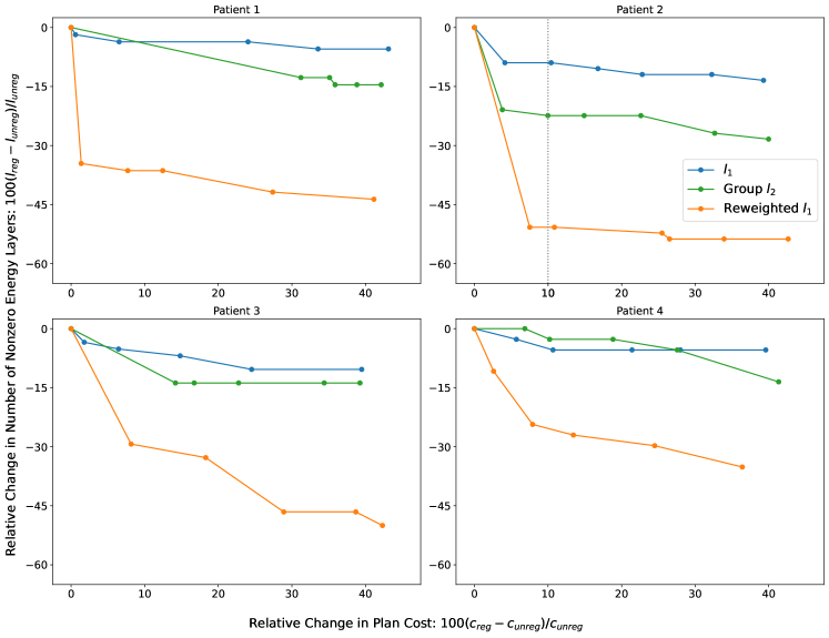
For every patient, Figure 5 depicts the relative percentage change in the number of nonzero spots versus the relative percentage change in plan cost for the $l_{1}$, group $l_{2}$, and reweighted $l_{1}$ regularization methods. The origin corresponds to the unregularized plan ($\lambda=0$). Both the $l_{1}$ and reweighted $l_{1}$ trade-off curves drop sharply from the origin, attaining on average a $30\%$ to $45\%$ decrease in nonzero spots for a less than $10\%$ increase in plan cost, with reweighted $l_{1}$ slightly outperforming $l_{1}$ by on average $5$ percentage points over all four patients. By contrast, the number of nonzero spots rises with group $l_{2}$ regularization, increasing up to $140\%$ within the first $10\%$ to $15\%$ increase in plan cost for all except patient $4$. This is consistent with our spot intensity plot for patient $2$ (Figure 1), which shows the spot distribution is denser under group $l_{2}$ than without regularization.

Figure 6 depicts the relative percentage change in the number of nonzero energy layers versus the relative percentage change in plan cost for the three regularization methods. Both $l_{1}$ and group $l_{2}$ trade-off curves decrease moderately from the origin, with group $l_{2}$ averaging about $9.5\%$ lower number of nonzero layers for a given percentage increase in cost. This matches our observations in Figures 2 and 3 that the group $l_{2}$ function is more effective at penalizing energy layers than the $l_{1}$ norm.

However, the reweighted $l_{1}$ method significantly outperforms both these regularizers. For patient $2$, it achieves an over $50\%$ decrease in the number of nonzero energy layers for a less than $10\%$ increase in plan cost. For the other patients, it provides a $25\%$ to $35\%$ reduction in active energy layers with a less than $15\%$ increment in plan cost. The average reduction in the number of nonzero layers from reweighted $l_{1}$ exceeds the best reduction from group $l_{2}$ by $12$ percentage points, and the majority of this reduction is realized with only about $10\%$ cost to treatment plan quality, relative to the unregularized plan.

The vertical dotted lines in Figures 5 and 6 for patient $2$ correspond to a $10\%$ increase in the plan cost. The intersection of these lines with the Pareto curves of different regularization methods demonstrates the reduction in the number of nonzero spots and energy layers obtained using different regularizers. Figure 7 (top right) depicts the dose-volume histogram (DVH) curves of the unregularized plan, the $l_{1}$ regularized plan, and the reweighted $l_{1}$ regularized plan at the same $10\%$ relative change in plan cost. (We chose not to show the DVHs of group $l_{2}$ regularized plans because they overlap considerably with the DVHs of corresponding $l_{1}$ regularized plans, and as we saw earlier, group $l_{2}$ results in far worse delivery efficiency than $l_{1}$ or reweighted $l_{1}$ regularization). Compared to no regularization, the reweighted $l_{1}$ method reduces the number of active spots and energy layers by more than $50\%$, while providing relatively similar DVH curves with different trade-offs (compromised left parotid and PTV coverage/homogeneity, and improved right parotid and mandible). One can re-adjust the PTV/OAR weights in the plan cost function of the reweighted $l_{1}$ problem to achieve more uniform trade-offs. In the same vein, compared to standard $l_{1}$ regularization, reweighted $l_{1}$ reduces the number of active spots and energy layers by about $10\%$ and $40\%$, respectively, while producing almost identical DVH curves. The Pareto curves and DVHs of the other patients, also plotted at roughly $10\%$ relative change in plan cost, tell a similar story.

The total plan delivery time is dependent on a multitude of machine-specific factors. In this section, we provide an estimate of how regularization directly impacts the delivery time, assuming a specific set of machine parameters. The total delivery time ($T$) can be approximated by

$$T=T_{b}\times(h_{b}(x)-1)_{+}+T_{e}\times(h_{e}(x)-1)_{+}+\sum_{g=1}^{G}T_{s}\times(h_{s}(x,\mathcal{I}_{g})-1)_{+}+\frac{\sum_{j=1}^{n}x_{j}}{T_{d}},$$

(13)

where $h_{b}(x)$ is the number of nonzero beams, $h_{e}(x)$ is the number of nonzero energy layers, $h_{s}(x,\mathcal{I}_{g})$ is the number of nonzero spots in energy layer $g$, $T_{b}$ is the beam switching time (gantry rotation plus beam setup time), $T_{e}$ is the energy layer switching time, $T_{s}$ is the spot travel time, and $T_{d}$ is the proton dose rate [GCM⁺20, ZSL⁺22]. Following van de Water et al. (2015) [vdWKHH15], we let $T_{b}=30$ seconds, $T_{e}=2$ seconds, $T_{s}=0.01$ seconds, and $T_{d}=\frac{4\times 10^{11}}{60}$ protons/second. We compute $T$ using the unregularized model and the $l_{1}$, group $l_{2}$, and reweighted $l_{1}$ regularized models, with regularization weight $\lambda$ chosen such that each regularized plan achieves a $10\%$ cost to plan quality. Then, we plot the relative percentage change in delivery time of each regularized model with respect to the unregularized model (i.e., $100(T_{reg}-T_{unreg})/T_{unreg}$).

The results for patient $2$ are shown in Figure 8. Standard $l_{1}$ reduces delivery time by a modest $13\%$, while group $l_{2}$ actually raises delivery time by $2\%$ due to the $149\%$ increase in the number of nonzero spots, which increases the spot delivery and spot travel time. By contrast, reweighted $l_{1}$ achieves a $44\%$ reduction in delivery time through its simultaneous reduction of the number of nonzero spots and nonzero energy layers by $57\%$ and $51\%$, respectively. This reduction comes at only a minor cost to the PTV and mandible – D$2\%$ to the PTV goes up by $4\%$ and maximum dose to the mandible goes up by $2\%$. Results for the other patients reflect similar outcomes, with reweighted $l_{1}$ reducing total delivery time by between $20\%$ and $30\%$; see Table 3 and Figure 9 in appendix B for additional data and plots.

References

- [AMNR02] M. Alber, G. Meedt, F. Nüsslin, and R. Reemtsen. On the degeneracy of the IMRT optimization problem. Med. Phys., 29(11):2584–2589, 2002.
- [AMT+12] L. M. Appenzoller, J. M. Michalski, W. L. Thorstad, S. Mutic, and K. L. Moore. Predicting dose-volume histograms for organs-at-risk in IMRT planning. Med. Phys., 39(12):7446–7461, 2012.
- [ApS22] MOSEK ApS. The MOSEK Optimizer API for Python, Version 10.0, 2022.
- [AVDB18] A. Agrawal, R. Verschueren, S. Diamond, and S. Boyd. A rewriting system for convex optimization problems. J. Control Decis., 5(1):42–60, 2018.
- [BdOCM] T. Bejarano, M. de Ornelas-Couto, and I. B. Mihaylov. Head-and-neck squamous cell carcinoma patients with CT taken during pre-treatment, mid-treatment, and post-treatment (HNSCC-3DCT-RT) [data set]. doi:10.7937/K9/TCIA.2018.13upr2xf.
- [BKM16] D. Bertsimas, A. King, and R. Mazumder. Best subset selection via a modern optimization lens. Ann. Stat., 44(2):813–852, 4 2016. doi:10.1214/15-AOS1388.
- [BPC+11] S. Boyd, N. Parikh, E. Chu, B. Peleato, , and J. Eckstein. Distributed optimization and statistical learning via the alternating direction method of multipliers. Found. Trends Mach. Learn., 3(1):1–122, 2011.
- [BSH09] S. Breedveld, P. Storchi, and B. Heijmen. The equivalence of multi-criteria methods for radiotherapy plan optimization. Phys. Med. Biol., 54(23):7199–7209, 2009.
- [BV04] S. Boyd and L. Vandenberghe. Convex Optimization. Cambridge University Press, 2004.
- [CB08] D. Craft and T. Bortfeld. How many plans are needed in an IMRT multi-objective plan database? Phys. Med. Biol., 53(11):2785–2796, 2008.
- [CLL+14] W. Cao, G. Lim, L. Liao, Y. Li, S. Jiang, X. Li, H. Li, K. Suzuki, X. R. Zhu, D. Gomez, and X. Zhang. Proton energy optimization and reduction for intensity-modulated proton therapy. Phys. Med. Biol., 59(21):6341–6354, 2014. doi:10.1088/0031-9155/59/21/6341.
- [CRT06] E. J. Candes, J. K. Romberg, and T. Tao. Stable signal recovery from incomplete and inaccurate measurements. Commun. Pure Appl. Math., 59(8):1207–1223, 2006.
- [CVS+13] K. Clark, B. Vendt, K. Smith, J. Freymann, J. Kirby, P. Koppel, S. Moore, S. Phillips, D. Maffitt, M. Pringle, L. Tarbox, and F. Prior. The cancer imaging archive (TCIA): Maintaining and operating a public information repository. J. Digit. Imaging, 26(6):1045–1057, 2013.
- [CWB08] E. J. Candés, M. B. Wakin, and S. P. Boyd. Enhancing sparsity by reweighted minimization. J. Fourier Anal. Appl., 14(1):877–905, 2008. doi:10.1007/s00041-008-9045-x.
- [DAM+22] S. Diamond, A. Agrawal, R. Murray, B. Stellato, and S. Boyd. CVXPY: Disciplined Convex Programming in Python, Version 1.3, 2022.
- [DB16] S. Diamond and S. Boyd. CVXPY: A Python-embedded modeling language for convex optimization. J. Mach. Learn. Res., 17(83):1–5, 2016.
- [DLZ+16] X. Ding, X. Li, M. Zhang, P. Kabolizadeh, C. Stevens, and D. Yan. Spot-scanning proton arc (SPArc) therapy: The first robust and delivery-efficient spot-scanning proton arc therapy. Int. J. Radiat. Oncol. Biol. Phys., 96(5):1107–1116, 12 2016. doi:10.1016/j.ijrobp.2016.08.049.
- [EBW+22] E. Engwall, C. Battinelli, V. Wase, O. Marthin, L. Glimelius, R. Bokrantz, B. Andersson, and A. Fredriksson. Fast robust optimization of proton PBS arc therapy plans using early energy layer selection and spot assignment. Phys. Med. Biol., 67(6):065010, 3 2022. doi:10.1088/1361-6560/ac55a6.
- [Faz02] M. Fazel. Matrix Rank Minimization with Applications. PhD thesis, Stanford University, 2002. https://faculty.washington.edu/mfazel/thesis-final.pdf.
- [FBDN07] M. Figueiredo, J. Bioucas-Dias, and R. D. Nowak. Majorization–minimization algorithms for wavelet-based image restoration. IEEE Trans. Image Process., 16(12):2980–2991, 12 2007. doi:10.1109/TIP.2007.909318.
- [FHB03] M. Fazel, H. Hindi, and S. Boyd. Log-det heuristic for matrix rank minimization with applications to hankel and euclidean distance matrices. In Proceedings of the American Control Conference (ACM), pages 2156–2162, Denver, CO, 6 2003. doi:10.1109/ACC.2003.1243393.
- [FTZ23] A. Fu, V. T. Taasti, and M. Zarepisheh. Distributed and scalable optimization for robust proton treatment planning. Med. Phys., 50(1):633–642, 1 2023. doi:10.1002/mp.15897.
- [FUXB19] A. Fu, B. Ungun, L. Xing, and S. Boyd. A convex optimization approach to radiation treatment planning with dose constraints. Optim. Eng., 20:277–300, 2019.
- [GCM+20] H. Gao, B. Clasie, M. McDonald, K. M. Langen, T. Liu, and Y. Lin. Technical note: Plan-delivery-time constrained inverse optimization method with minimum-MU-per-energy-layer (MMPEL) for efficient pencil beam scanning proton therapy. Med. Phys., 47(9):3892–3897, 9 2020.
- [Gor22] B. L. Gorissen. Interior point methods can exploit structure of convex piecewise linear functions with application in radiation therapy. SIAM J. Optim., 32(1):256–275, 2022. doi:10.1137/21M1402364.
- [GRL+20] W. Gu, D. Ruan, Q. Lyu, W. Zou, L. Dong, and K. Sheng. A novel energy layer optimization framework for spot-scanning proton arc therapy. Med. Phys., 47(5):2072–2084, 2 2020. doi:10.1002/mp.14083.
- [HTW15] T. Hastie, R. Tibshirani, and M. Wainwright. Statistical Learning with Sparsity: The Lasso and Generalizations. Monographs on Statistics and Applied Probability. Taylor and Francis, 2015.
- [IPR16] S. Ivanoff, F. Picard, and V. Rivoirard. Adaptive lasso and group-lasso for functional Poisson regression. J. Mach. Learn. Res., 17(1):1903–1948, 2016.
- [JHP+18] M. F. Jensen, L. Hoffmann, J. B. B. Petersen, D. S. Møller, and M. Alber. Energy layer optimization strategies for intensity-modulated proton therapy of lung cancer patients. Med. Phys., 45(10):4355–4363, 10 2018. doi:10.1002/mp.13139.
- [JOV09] L. Jacob, G. Obozinski, and J.-P. Vert. Group lasso with overlap and graph lasso. In Proceedings of the International Conference on Machine Learning (ICML), pages 433–440, Montreal, Canada, 6 2009. doi:10.1145/1553374.1553431.
- [LASP04] J. Llacer, N. Agazaryan, T. D. Solberg, and C. Promberger. Degeneracy, frequency response and filtering in IMRT optimization. Phys. Med. Biol., 49(13):2853–2880, 2004.
- [LCL+19] Y. Lin, B. Clasie, T. Liu, M. McDonald, K. M. Langen, and H. Gao. Minimum-MU and sparse-energy-layer (MMSEL) constrained inverse optimization method for efficiently deliverable PBS, plans. Phys. Med. Biol., 64(20):205001, 2019. doi:10.1088/1361-6560/ab4529.
- [LFB07] M. S. Lobo, M. Fazel, and S. Boyd. Portfolio optimization with linear and fixed transaction costs. Ann. Oper. Res, 152(1):341–365, 2007. doi:10.1007/s10479-006-0145-1.
- [LH15] M. Lim and T. Hastie. Learning interactions via hierarchical group-lasso regularization. J. Comput. Graph. Stat., 24(3):627–654, 2015. doi:10.1080/10618600.2014.938812.
- [LLZ+20] G. Liu, X. Li, L. Zhao, W. Zheng, A. Qin, S. Z hang, C. Stevens, D. Yan, P. Kabolizadeh, and X. Ding. A novel energy sequence optimization algorithm for efficient spot-scanning proton arc (SPArc) treatment delivery. Acta Oncol., 59(10):1178–1185, 2020. doi:10.1080/0284186X.2020.1765415.
- [LZZ15] H. Li, X. R. Zhu, and X. Zhang. Reducing dose uncertainty for spot-scanning proton beam therapy of moving tumors by optimizing the spot delivery sequence. Int. J. Radiat. Oncol. Biol. Phys., 93(3):547–556, 2015. doi:10.1016/j.ijrobp.2015.06.019.
- [Mai15] J. Mairal. Incremental majorization-minimization optimization with application to large-scale machine learning. SIAM J. Optim., 25(2):829–855, 2015. doi:10.1137/140957639.
- [MCN+20] D. Mah, C. C. Chen, A. O. Nawaz, G. Galbreath, R. Shmulenson, N. Lee, and B. Chon. Retrospective analysis of reduced energy switching and room switching times on throughput efficiency of a multi-room proton therapy center. Brit. J. Radiol., 93(1107):20190820, 3 2020. doi:10.1259/bjr.20190820.
- [MHDZ20] S. Mukherjee, L. Hong, J. O. Deasy, and M. Zarepisheh. Integrating soft and hard dose-volume constraints into hierarchical constrained IMRT optimization. Med. Phys., 47(2):414–421, 2020.
- [MKBT08] M. Monz, K.-H. Küfer, T. Bortfeld, and C. Thieke. Pareto navigation—algorithmic foundation of interactive multi-criteria IMRT planning. Phys. Med. Biol., 53(4):985–998, 2008.
- [MSH07] S. Ma, X. Song, and J. Huang. Supervised group lasso with applications to microarray data analysis. BMC Bioinform., 8(60):1–17, 2 2007. doi:10.1186/1471-2105-8-60.
- [MvdGB08] L. Meier, S. van de Geer, and P. Bühlmann. The group lasso for logistic regression. J. R. Stat. Soc., B: Stat. Methodol., 70(1):53–71, 2 2008. doi:10.1111/j.1467-9868.2007.00627.x.
- [MW16] B. S. Müller and J. J. Wilkens. Prioritized efficiency optimization for intensity modulated proton therapy. Phys. Med. Biol., 61(23):8249–8265, 2016. doi:10.1088/0031-9155/61/23/8249.
- [NW06] J. Nocedal and S. J. Wright. Numerical Optimization. Springer-Verlag, 2006.
- [Pag12] H. Paganetti. Range uncertainties in proton therapy and the role of Monte Carlo simulations. Phys. Med. Biol., 57(11):R99–R117, 2012.
- [PEL+18] P. R. Poulsen, J. Eley, U. Langner, II C. B. Simone, and K. Langen. Efficient interplay effect mitigation for proton pencil beam scanning by spot-adapted layered repainting evenly spread out over the full breathing cycle. Int. J. Radiat. Oncol. Biol. Phys., 100(1):226–234, 1 2018.
- [PH07] M. Y. Park and T. Hastie. -regularization path algorithm for generalized linear models. J. R. Stat. Soc., B: Stat. Methodol., 69(4):659–677, 9 2007. doi:10.1111/j.1467-9868.2007.00607.x.
- [PSL17] D. Petrova, S. Smickovska, and E. Lazarevska. Conformity index and homogeneity index of the postoperative whole breast radiotherapy. Open Access Maced. J. Med. Sci., 5(6):736–739, 2017.
- [QSG13] Z. Qin, K. Scheinberg, and D. Goldfarb. Efficient block-coordinate descent algorithms for the group lasso. Math. Program. Comput., 5(2):143–169, 6 2013. doi:10.1007/s12532-013-0051-x.
- [Rak11] A. Rakotomamonjy. Surveying and comparing simultaneous sparse approximation (or group-lasso) algorithms. Signal Process., 91(7):1505–1526, 7 2011. doi:10.1016/j.sigpro.2011.01.012.
- [SBP17] Y. Sun, P. Babu, and D. P. Palomar. Majorization-minimization algorithms in signal processing, communications, and machine learning. IEEE Trans. Signal Process., 65(3):794–816, 2 2017.
- [SFR07] M. Schmidt, G. Fung, and R. Rosales. Fast optimization methods for regularization: A comparative study and two new approaches. In European Conference on Machine Learning (ECML), pages 286–297, Warsaw, Poland, 9 2007.
- [SNZ+20] C. Shen, D. Nguyen, Z. Zhou, S. B. Jiang, B. Dong, and X. Jia. An introduction to deep learning in medical physics: Advantages, potential, and challenges. Phys. Med. Biol., 65(5):05TR01, 2020.
- [SPS+16] K. Suzuki, M. B. Palmer, N. Sahoo, X. Zhang, F. Poenisch, D. S. Mackin, A. Y. Liu, R. Wu, X. R. Zhu, S. J. Frank, M. T. Gillin, and A. K. Lee. Quantitative analysis of treatment process time and throughput capacity for spot scanning proton therapy. Med. Phys., 43(7):3975–3986, 7 2016.
- [SSW10] E. D. Schifano, R. L. Strawderman, and M. T. Wells. Majorization-minimization algorithms for nonsmoothly penalized objective functions. Electron. J. Stat., 4(1):1258–1299, 2010. doi:10.1214/10-EJS582.
- [ST12] N. Simon and R. Tibshirani. Standardization and the group lasso. Stat. Sin., 22(3):983–1001, 7 2012. doi:10.5705/ss.2011.075.
- [SYOS10] J. Shi, W. Yin, S. Osher, and P. Sajda. A fast hybrid algorithm for large-scale -regularized logistic regression. J. Mach. Learn. Res., 11(23):713–741, 2010.
- [TBD+18] V. T. Taasti, C. Bäumer, C. V. Dahlgren, A. J. Deisher, M. Ellerbrock, J. Free, J. Gora, A. Kozera, A. J. Lomax, L. De Marzi, S. Molinelli, B.-K. K. Teo, P. Wohlfahrt, J. B. B. Petersen, L. P. Muren, D. C. Hansen, and C. Richter. Inter-centre variability of CT-based stopping-power prediction in particle therapy: Survey-based evaluation. Phys. Imaging Radiat., 6(1):25–30, 2018.
- [THDZ20] V. T. Taasti, L. Hong, J. O. Deasy, and M. Zarepisheh. Automated proton treatment planning with robust optimization using constrained hierarchical optimization. Med. Phys., 47(7):2779–2790, 2020.
- [THS+20] V. T. Taasti, L. Hong, J. S. Shim, J. O. Deasy, and M. Zarepisheh. Automating proton treatment planning with beam angle selection using bayesian optimization. Med. Phys., 47(8):3286–3296, 8 2020. doi:10.1002/mp.14215.
- [Tib96] R. Tibshirani. Regression shrinkage and selection via the lasso. J. R. Stat. Soc., B: Stat. Methodol., 58(1):267–288, 1996.
- [VBL13] D. Vidaurre, C. Bielza, and P. Larrañaga. A survey of regression. Int. Stat. Rev., 81(3):361–381, 12 2013.
- [vdWBA+20] S. van de Water, M. F. Belosi, F. Albertini, C. Winterhalter, D. C. Weber, and A. J. Lomax. Shortening delivery times for intensity-modulated proton therapy by reducing the number of proton spots: An experimental verification. Phys. Med. Biol., 65(9):095008, 5 2020. doi:10.1088/1361-6560/ab7e7c.
- [vdWKHH15] S. van de Water, H. M. Kooy, B. J. M. Heijmen, and M. S. Hoogeman. Shortening delivery times of intensity modulated proton therapy by reducing proton energy layers during treatment plan optimization. Int. J. Radiat. Oncol. Biol. Phys., 92(2):460–468, 2015. doi:10.1016/j.ijrobp.2015.01.031.
- [WCW+17] H.-P. Wieser, E. Cisternas, N. Wahl, S. Ulrich, A. Stadler, H. Mescher, L.-R. Müller, T. Klinge, H. Gabrys, L. Burigo, A. Mairani, S. Ecker, B. Ackermann, M. Ellerbrock, K. Parodi, O. Jäkel, and M. Bangert. Development of the open-source dose calculation and optimization toolkit matRad. Med. Phys., 44(6):2556–2568, 2017.
- [WL08] T. T. Wu and K. Lange. Coordinate descent algorithms for lasso penalized regression. Ann. Appl. Stat., 2(1):224–244, 2008. doi:10.1214/07-AOAS147.
- [Wri97] S. J. Wright. Primal-Dual Interior Point Methods. Society for Industrial and Applied Mathematics, 1997.
- [WSGJ+22] S. Wuyckens, M. Saint-Guillain, G. Janssens, L. Zhao, X. Li, X. Ding, E. Sterpin, J. A. Lee, and K. Souris. Treatment planning in arc proton therapy: Comparison of several optimization problem statements and their corresponding solvers. Comput. Biol. Med., 148(1):105609, 9 2022. doi:10.1016/j.compbiomed.2022.105609.
- [WWG+18] H.P. Wieser, N. Wahl, H.S. Gabryś, L.R. Müller, G. Pezzano, J. Winter, S. Ulrich, L. Burigo, O. Jäkel, and M. Bangert. MatRad – an open-source treatment planning toolkit for educational purposes. Med. Phys. Int., 6(1):119–127, 2018.
- [WZSG+22] S. Wuyckens, L. Zhao, M. Saint-Guillain, G. Janssens, E. Sterpin, K. Souris, X. Ding, and J. A. Lee. Bi-criteria Pareto optimization to balance irradiation time and dosimetric objectives in proton arc therapy. Phys. Med. Biol., 67(1):245017, 12 2022. doi:10.1088/1361-6560/aca5e9.
- [YL06] M. Yuan and Y. Lin. Model selection and estimation in regression with grouped variables. J. R. Stat. Soc., B: Stat. Methodol., 68(1):49–67, 2 2006. doi:10.1111/j.1467-9868.2005.00532.x.
- [YZ15] Y. Yang and H. Zou. A fast unified algorithm for solving group-lasso penalized learning problems. Stat. Comput., 25(1):1129–1141, 2015. doi:10.1007/s11222-014-9498-5.
- [ZHZ+22] M. Zarepisheh, L. Hong, Y. Zhou, Q. Huang, J. Yang, G. Jhanwar, H. D. Pham, P. Dursun, P. Zhang, M. A. Hunt, G. S. Mageras, J. T. Yang, Y. Yamada, and J. O. Deasy. Automated and clinically optimal treatment planning for cancer radiotherapy. INFORMS J. Appl. Anal., 52(1):69–89, 2022.
- [ZSL+22] G. Zhang, H. Shen, Y. Lin, R. C. Chen, Y. Long, and H. Gao. Energy layer optimization via energy matrix regularization for proton spot-scanning arc therapy. Med. Phys., 49(9):5752–5762, 9 2022. doi:10.1002/mp.15836.
- [ZST+13] M. Zarepisheh, M. Shakourifar, G. Trigila, P. S. Ghomi, S. Couzens, A. Abebe, L. Noreña, W. Shang, S. B. Jiang, and Y. Zinchenko. A moment-based approach for DVH-guided radiotherapy treatment plan optimization. Phys. Med. Biol., 58(6):1869–1887, 2013.
Appendix A Derivation of problem 3
Problem 2 in the main text is a nonconvex optimization problem because the equality constraints and are nonlinear. We will show that it is equivalent to the convex optimization problem 3, which replaces the nonlinear equality constraints with the linear equality constraint . Since the objective functions are identical, it is sufficient to prove that any solution of problem 2 is a feasible point for problem 3 and vice versa.
Let be a solution of problem 2. Then,
because any real function can be written as the sum of its nonnegative and nonpositive parts. Thus, is feasible for problem 3, and since the two problems have the same objective function, is a solution of problem 3.
Now let us show the converse. First, we will relax the equality constraints in problem 2 to get