Simultaneous Navigation and Radio Mapping
for Cellular-Connected UAV
with Deep Reinforcement Learning
Abstract
Cellular-connected unmanned aerial vehicle (UAV) is a promising technology to unlock the full potential of UAVs in the future by reusing the cellular base stations (BSs) to enable their air-ground communications. However, how to achieve ubiquitous three-dimensional (3D) communication coverage for the UAVs in the sky is a new challenge. In this paper, we tackle this challenge by a new coverage-aware navigation approach, which exploits the UAV’s controllable mobility to design its navigation/trajectory to avoid the cellular BSs’ coverage holes while accomplishing their missions. To this end, we formulate an UAV trajectory optimization problem to minimize the weighted sum of its mission completion time and expected communication outage duration, which, however, cannot be solved by the standard optimization techniques mainly due to the lack of an accurate and tractable end-to-end communication model in practice. To overcome this difficulty, we propose a new solution approach based on the technique of deep reinforcement learning (DRL). Specifically, by leveraging the state-of-the-art dueling double deep Q network (dueling DDQN) with multi-step learning, we first propose a UAV navigation algorithm based on direct RL, where the signal measurement at the UAV is used to directly train the action-value function of the navigation policy. To further improve the performance, we propose a new framework called simultaneous navigation and radio mapping (SNARM), where the UAV’s signal measurement is used not only for training the DQN directly, but also to create a radio map that is able to predict the outage probabilities at all locations in the area of interest. This thus enables the generation of simulated UAV trajectories and predicting their expected returns, which are then used to further train the DQN via Dyna technique, thus greatly improving the learning efficiency. Simulation results demonstrate the effectiveness of the proposed algorithms for coverage-aware UAV navigation, as well as the significantly improved performance of SNARM over direct RL.
I Introduction
Conventionally, cellular networks are designed to mainly serve terrestrial user equipments (UEs) with fixed infrastructure. With the continuous expansion of human activities towards the sky and the fast growing use of unmanned aerial vehicles (UAVs) for various applications, there have been increasing interests in integrating UAVs into cellular networks [2]. On one hand, dedicated UAVs could be dispatched as aerial base stations (BSs) or relays to assist wireless communications between devices without direct connectivity, or as flying access points (APs) for data collection and information dissemination, leading to a new three-dimensional (3D) network with UAV-assisted communications [3]. On the other hand, for those UAVs with their own missions, cellular network could be utilized to support their command and control (C&C) communication as well as payload data transmissions, corresponding to the other paradigm of cellular-connected UAV [4]. In particular, by reusing the existing densely deployed cellular BSs worldwide, together with the advanced cellular technologies, cellular-connected UAV has the great potential to achieve truly remote UAV operation with unlimited range, not to mention other advantages such as the ease of legitimate UAV monitoring and management, high-capacity payload transmission, and cellular-enhanced positioning [2, 4].
However, to practically realize the above vision of cellular-connected UAVs, there are still several critical challenges to be addressed. In particular, as existing cellular networks are mainly planned for ground coverage with BS antennas typically downtilted towards the ground [5], unlike that on the ground, ubiquitous cellular coverage in the sky cannot be guaranteed in general [6]. In fact, even for the forthcoming 5G or future 6G cellular networks that are planned to embrace the new type of aerial UEs, it is still unclear whether ubiquitous sky coverage is economically viable or not, even for some moderate range of altitude, considering various practical factors such as infrastructural and operational costs, as well as the anticipated aerial UE density in the near future. Such coverage issue is exacerbated by the more severe aerial-ground interference as compared to the terrestrial counterpart [6, 7, 4], due to the high likelihood of having strong line of sight (LoS) channels for the UAVs with their non-associated co-channel BSs.
Fortunately, different from the conventional ground UEs whose mobility is typically random and uncontrollable, which renders ubiquitous ground coverage essential, the mobility of UAVs is more predictable and most of the time controllable, either autonomously by computer program or by remote pilots. This thus offers a new degree of freedom to circumvent the aforementioned coverage issue, via coverage-aware navigation or trajectory design: an approach that requires no or little modifications for cellular networks to serve aerial UEs. There are some preliminary efforts along this direction. In [8], by applying graph theory and convex optimization for cellular-connected UAV, the UAV trajectory is optimized to minimize the UAV travelling time while ensuring that it is always connected with at least one BS. A similar problem is studied in [9, 10], by allowing certain tolerance for disconnection.
However, the conventional optimization-based UAV trajectory design like those mentioned above have practical limitations. First, formulating the corresponding optimization problems requires accurate and analytically tractable end-to-end communication models, including the BS antenna model, channel model, interference model and even local environmental model. Perhaps for such reasons, prior works such as [8, 9, 10] have mostly assumed some simplified models like isotropic radiation for antennas and/or free-space path loss channel model for aerial-ground links. Although there have been previous works considering more sophisticated channel models, like the probabilistic LoS channel model [11] and angle-dependent channel parameters [12, 13], these are statistical models that can only predict the performance in the average sense without providing any performance guarantee for the local environment where the UAVs are actually deployed. Another limitation of off-line optimization-based trajectory design is the requirement of perfect and usually global knowledge of the channel model parameters, which is difficult to acquire in practice. Last but not least, even with the accurate channel model and the perfect information of all relevant parameters, most of these off-line optimization problems are highly non-convex and thus difficult to be efficiently solved.
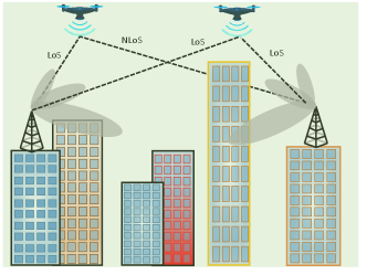
To overcome the above limitations, we propose in this paper a new approach for coverage-aware UAV navigation based on reinforcement learning (RL) [14], which is one type of machine learning techniques for solving sequential decision problems. As shown in Fig. 1, we consider a typical cellular-connected UAV system in urban environment, where multiple UAVs need to operate in a given airspace with their communications supported by cellular BSs. The UAV missions are to fly from their respective initial locations to a common final location with minimum time,111The results of this paper can be extended to the general case of different final locations for the UAVs. while maintaining a satisfactory communication connectivity with the cellular network with best effort. Our main contributions are summarized as follows:
-
•
First, we formulate the UAV trajectory optimization problem to minimize the weighted sum of its mission completion time and the expected communication outage duration, which, however, is difficult to be solved via the standard optimization techniques mainly due to the lack of an accurate and tractable communication model. Fortunately, we show that the formulated problem can be transformed to an equivalent Markov decision process (MDP), for which a handful of RL techniques, such as the classic Q learning [14], can be applied to learn the UAV action policy, or the flying direction in our problem.
-
•
As the resulting MDP involves continuous state space that essentially has infinite number of state-action pairs and thus renders the simple table-based Q learning inapplicable, we apply the celebrated deep neural network (DNN) to approximate the action-value function (or Q function), a technique commonly known as deep reinforcement learning (DRL) or more specifically, deep Q learning [15]. To train the DNN, we use the state-of-the-art dueling network architecture with double DQN (dueling DDQN) [16] and multi-step learning. Different from the conventional off-line optimization-based designs, the proposed DRL-based trajectory design does not require any prior knowledge about the channel model or propagation environment, but only utilizes the raw signal measurement at each UAV as the input to improve its radio environmental awareness, as evident from the continuously improved estimation accuracy of the UAVs’ action-value functions.
-
•
As direct RL based on real experience or measured data only is known to be data inefficient, i.e., a large amount of data or agent-environment interaction is needed, we further propose a new design framework termed simultaneous navigation and radio mapping (SNARM) to improve the learning efficiency. Specifically, with SNARM, the network (say, a macrocell BS in the area of interest) maintains a database, also known as radio map [17, 18], which provides the outage probability distribution over the space of interest with respect to the relatively stable (large-scale) channel parameters. As such, the obtained signal measurements as UAVs fly along their trajectories are used for dual purposes: to train the DQN to improve the estimation of the optimal action-value functions, as well as to improve the accuracy of the estimated radio map, which is used for the prediction of the outage probability for other locations in the considered area even if they have not been visited by any UAV yet. The exploitation of the radio map, whose accuracy is continuously improved as more signal measurements are accumulated, makes it possible to generate simulated UAV trajectories and predict their corresponding returns, without having to actually fly the UAVs along them. This thus leads to our proposed SNARM framework, by applying the classic Dyna [14] dueling DDQN with multi-step learning to train the action-value functions with a combined use of real trajectories and simulated trajectories, thus greatly reducing the actual UAV flights or measurement data required.
-
•
Numerical results are provided, with the complete source codes available online222https://github.com/xuxiaoli-seu/SNARM-UAV-Learning, to verify the performance of the proposed algorithms. It is observed that the SNARM algorithm is able to learn the radio map very efficiently, and both direct RL and SNARM algorithms are able to effectively navigate UAVs to avoid the weak coverage regions of the cellular network. Furthermore, thanks to the simultaneous learning of the radio map, SNARM is able to significantly reduce the number of required UAV flights (or learning episodes) than direct RL while achieving comparable performance.
Note that applying RL techniques for UAV communications has received significant attention recently [19, 20, 21, 22, 23] and DRL has also been used in wireless networks [24] for solving various problems like multiple access control [25], power allocation [26], modulation and coding [27], mobile edge computing [28], UAV BS placement [29], and UAV interference management [30], among others. On the other hand, local environmental-aware UAV path/trajectory design has been studied from different perspectives, such as that based on the known radio map [31] or 3D city map [32, 33], or the joint online and off-line optimization for UAV-enabled data harvesting [34]. Compared to such existing path/trajectory designs, the proposed coverage-aware navigation algorithms based on direct RL or SNARM do not require any prior knowledge or assumption about the environment, but only utilize the UAV’s measured data as the input for action and/or radio map learning, thus expected to be more robust to any imperfect knowledge or change of the local environment. Although large data measurements are generally required for the proposed algorithms, they are practically available according to the existing cellular communication protocols, such as the reference signal received power (RSRP) and reference signal received quality (RSRQ) measurements. Besides, as different UAVs in the same region share the same local radio propagation environment, regardless of operating concurrently or at different time, their measured data as they perform their respective missions can actually be collectively utilized for our proposed designs, to continuously improve the quality of the learning for the future missions, which thus greatly alleviates the burden for data acquisition in practice.
The rest of the paper is organized as follows. Section II introduces the system model and problem formulation. In Section III, we give a very brief background about RL and DRL, mainly to introduce the key concepts and main notations. Section IV presents the proposed algorithms, including the direct RL based on dueling DDQN with multi-step learning for UAV navigation, and SNARM to enable path learning with both real and simulated flight experience. Section V presents the numerical results, and finally we conclude the paper in Section VI.
II System Model and Problem Formulation
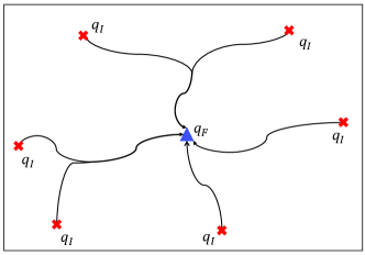
As shown in Fig. 1, we consider a cellular-connected UAV system with arbitrary number of UAV users. Without loss of generality, we assume that the airspace of interest is a cubic volume, which is specified by , with the subscripts and respectively denoting the lower and upper bounds of the 3D coordinate of the airspace. UAVs with various missions need to operate in this airspace with communications supported by cellular BSs. While different UAVs usually have different missions and may operate at different time, since they share the common airspace, their flight experience including their signal measurements along their respective flying trajectories, can be exploited collectively to improve their radio environmental awareness. To make the problem concrete, we consider the scenario that the UAVs need to fly from their respective initial locations , which are generally different for different UAVs, to a common final location , as shown in Fig. 2. This setup corresponds to various UAV applications such as UAV-based parcel collection, with corresponding to the customer’s home location and being the local processing station of courier company, or UAV-based aerial inspection, with being the target point for inspection and being the charging station in the local area, etc. We assume that collision/obstacle avoidance is guaranteed by e.g., ensuring that UAVs are sufficiently separated in operation time or space, and their flight altitudes are higher than the maximum building height. Without loss of generality, we can focus on one typical UAV, since other UAVs may apply similar strategies to update the common location-dependent database, such as the action-value function of the RL algorithms and the radio map of the environment (to be defined later). The UAV needs to be navigated from its initial location to the final location with the minimum mission completion time, while maintaining a satisfactory communication connectivity with the cellular network. Let denote the mission completion time and , , represent the UAV trajectory. Then we should have
| (1) | |||
| (2) |
where and , with denoting the element-wise inequality.
Let denote the total number of cells in the area of interest, and , , represent the baseband equivalent channel from cell to the UAV at time , which generally depends on the BS antenna gains, the large-scale path loss and shadowing that are critically dependent on the local environment, as well as the small-scale fading. The received signal power at time by the UAV from cell can be written as
| (3) | ||||
| (4) |
where denotes the transmit power of cell that is assumed to be a constant, and denote the large-scale channel gain and the BS antenna gain, respectively, which generally depend on the UAV location , and is a random variable accounting for the small-scale fading. As the proposed designs in this paper work for arbitrary channels, a detailed discussion of one particular BS-UAV channel model adopted for our simulations is deferred to Section V.
Denote by the cell associated to the UAV at time . We say that the UAV is in outage at time if its received signal-to-interference ratio (SIR) is below a certain threshold , i.e., when , where
| (5) |
Note that for simplicity, we have ignored the noise effect, since BS-UAV communication is known to suffer from more severe interference than the terrestrial counterparts, and thus its communication performance is usually interference-limited. Besides, we consider the worst-case scenario with universal frequency reuse so that all these non-associated BSs would contribute to the sum-interference term in (5). The extension of the proposed techniques for dynamic interference will be an interesting work for further investigation.
Due to the randomness of small-scale fading, for any given UAV location and cell association at time , in (5) is a random variable, and the resulting outage probability is a function of and , i.e.,
| (6) |
where is the probability of the event taken with respect to the randomness of small-scale fading . Then the total expected outage duration across the UAV’s mission duration is
| (7) |
Intuitively, with longer mission completion time , the UAV is more flexible to adapt its trajectory to avoid the weak coverage regions of the cellular network in the sky and thus reduce the expected outage duration . Therefore, there in general exists a tradeoff between minimizing the mission completion time and expected outage duration , which can be balanced by designing and to minimize the weighted sum of these two metrics with certain weight , as formulated in the following optimization problem.
| (8) | ||||
| (9) | ||||
| (10) | ||||
| (11) |
where denotes the maximum UAV speed. It can be shown that at the optimal solution to , the UAV should fly with the maximum speed , i.e., , where denotes the UAV flying direction with . Thus, can be equivalently written as
| (12) | ||||
| (13) | ||||
In practice, finding the optimal UAV trajectory and cell association by directly solving the optimization problem faces several challenges. First, to complete the problem formulation of to make it ready for optimization, we still need to derive the closed-form expression for the expected outage duration for any given UAV location and association , which is challenging, if not impossible. On one hand, this requires accurate and tractable modelling of the end-to-end channel for cellular-UAV communication links, where practical 3D BS antenna pattern [35] and the frequent variations of LoS/NLoS connections, which depends on the actual building/terrain distributions in the area of interest, need to be considered. On the other hand, even with such modelling and the perfect knowledge of the terrain/building information for the area of interest, deriving the closed-form expression for is mathematically difficult since the probability density function (pdf) of the SIR depends on the UAV trajectory in sophisticated manners, as can be inferred from (4) and (5). Furthermore, even after completing the problem formulation of with properly defined cost function, the resulting optimization problem will be highly non-convex and difficult to be efficiently solved.
To overcome the above issues, in the following, we propose a novel approach for coverage-aware UAV navigation by leveraging the powerful mathematical framework of RL and DNN, which only requires the UAV signal measurements along its flight as the input. By leveraging the state-of-the-art dueling DDQN with multi-step learning [36], we first propose the direct RL-based algorithm for coverage-aware UAV navigation, and then introduce the more advanced SNARM algorithm to improve the learning efficiency and UAV performance.
III Overview of Deep Reinforcement Learning
This section aims to give a brief overview on RL and DRL, by introducing the key notations to be used in the sequel of this paper. The readers are referred to the classic textbook [14] for a more comprehensive description.
III-A Basics of Reinforcement Learning
RL is a useful machine learning method to solve the MDP [14], which consists of an agent interacting with the environment iteratively. For the fully observable MDP, at each discrete time step , the agent observes a state , takes an action , and then receives an immediate reward and transits to the next state . Mathematically, an MDP can be specified by 4-tuple , where is the state space, is the action space, is the state transition probability, with specifying the probability of transiting to the next state given the current state after applying the action , and is the immediate reward received by the agent, usually denoted by for reward received at time step or to show its general dependency on and .
The agent’s actions are governed by its policy , where gives the probability of taking action when in state . The goal of the agent is to improve its policy based on its experience, so as to maximize its long-term expected return , where the return is the accumulated discounted reward from time step onwards with a discount factor .
A key metric of RL is the action-value function, denoted as , which is the expected return starting from state , taking the action , and following policy thereafter, i.e., . The optimal action-value function is defined as , and . If the optimal value function is known, the optimal policy can be directly obtained as
| (14) |
Thus, an essential task of RL is to obtain the optimal value functions, which satisfy the celebrated Bellman optimality equation [14]
| (15) |
Bellman optimality equation is non-linear, and admits no closed-form solution in general. However, many iterative solutions have been proposed. Specifically, when the agent has the full knowledge of the MDP, including the reward and the state-transition probabilities , the optimal value function can be obtained recursively based on dynamic programming, such as value iteration [14]. On the other hand, when the agent has no or incomplete prior knowledge about the MDP, it may apply the useful idea of temporal difference (TD) learning to improve its estimation of the value function by directly interacting with the environment. Specifically, TD learning is a class of model-free RL methods that learn the value functions based on the direct samples of the state-action-reward-nextState sequence, with the estimation of the value functions updated by the concept of bootstrapping. One classic TD learning method is Q-learning, which applies the following update to the action-value function with the observed sample reward-and-state transitions :
where is the learning rate. It has been shown that Q-learning is able to converge to the optimal action-value function if each state-action pair is visited by sufficient times and appropriate learning rate is chosen [14].
III-B Deep Reinforcement Learning
The RL learning method discussed in Section III-A is known as table-based, which requires storing one value for each state-action pair, and the value is updated only when that state-action pair is actually experienced. This becomes impractical for continuous state/action or when the number of discretized states/actions is very large. In order to practically apply RL algorithms to large/continuous state-action space, one may resort to the useful technique of function approximation [14], where the action-value function is approximated by certain parametric function, e.g., , , with a parameter vector . Function approximation brings two advantages over table-based RL. Firstly, instead of storing and updating the value functions for all state-action pairs, one only needs to learn the parameter , which typically has much lower dimension than the number of state-action pairs. Secondly, function approximation enables generalization, i.e., the ability to predict the values even for those state-action pairs that have never been experienced, since different state-action pairs are coupled with each other via the function and parameter .
One powerful non-linear function approximation technique is via using artificial neural networks (ANNs), which are networks consisting of interconnected units (or neurons), with each unit computing a weighted sum of their input signals and then applying a nonlinear function (called the activation function) to produce its output. It has been theoretically shown that an ANN with even a single hidden layer containing a sufficiently large number of neurons is a universal function approximation [14], i.e., it can approximate any continuous function on a compact region to any degree of accuracy. Nonetheless, researchers have found that ANNs with deep architectures consisting of many hidden layers are of more practical usage for complex function approximations. A combination of RL with function approximation based on deep ANNs leads to the powerful framework of DRL [15].
With deep ANN for the action-value function approximation , the parameter vector actually corresponds to the weight coefficients and bias of all links in the ANNs. In principle, can be updated based on the classic backpropagation algorithm [37]. However, its application for DRL faces new challenges, since standard ANNs are usually trained in the supervised learning manner, i.e., the labels (in this case the true action values) of the input training data are known, which is obviously not the case for DRL. This issue can be addressed by the idea of bootstrapping, i.e., for each given state-action-reward-nextState transition , the parameter of the network is updated to minimize the loss given by
| (16) |
However, as the target in (16) also depends on the parameter to be actually updated, directly applying the standard deep training algorithms with (16) can lead to oscillations or even divergence. This problem was addressed in the celebrated work [15], which proposed the simple but effective technique of “target network” to bring the Q-learning update closer to the standard supervised-learning setup. A target network, denoted as with parameter , is a copy of the Q network , but with its parameter updated much less frequently. For example, after every number of updates to the weights of the Q network, we may set equal to and keep it unchanged for the next updates of . Thus, the loss in (16) is modified to
| (17) |
This helps to keep the target remaining relatively stable and hence improve the convergence property of the training.
Another essential technique proposed in [15] is experience replay, which stores the state-action-reward-nextState transition into a replay memory and then randomly access them later to perform the weight updates. Together with mini-batch update, i.e., multiple experiences are sampled uniformly at random from the replay memory for each update, experience replay helps to reduce the variance of the updates by avoiding highly correlated data for successive updates.
Soon after the introduction of DQN in [15], many techniques for further performance improvement have been proposed, such as DDQN [38] to address the over-estimation bias of the maximum operation of the Q learning, DQN with prioritized experience replay (PER) [39], DQN with the dueling network architecture [16], and a combination of all major improvement techniques, termed Rainbow, has been introduced in [36].
IV Proposed Algorithms
In this section, we present our proposed DRL-based algorithms for solving the coverage-aware UAV navigation problem (P1).
IV-A Coverage-Aware UAV Navigation as an MDP
The first step to apply RL algorithms for solving a real-world problem is to reformulate it as an MDP. As MDP is defined over discrete time steps, for the UAV navigation and cell association problem , we need to first discretize the time horizon into time steps with certain interval , where . Note that should be small enough so that within each time step, the distance between the UAV and any BS in the area of interest are approximately unchanged, or their large-scale channel gain and the BS antenna gain towards the UAV, i.e., and in (4), remain approximately constant. As such, the UAV trajectory can be approximately represented by the sequence , thus (12) and (13) can be rewritten as
| (18) | |||
| (19) |
where is the UAV (maximum) displacement per time step, and denotes the UAV flying direction at time step . Furthermore, as cell association is usually based on large-scale channel gains with BSs to avoid too frequent handover, the associated cell thus remains unchanged within each time step. Thus, the association policy can be represented in discrete time as . As a result, the expected outage duration (7) can be approximately rewritten as
| (20) |
For each time step with given UAV location and cell association , deriving a closed-form expression for is difficult as previously mentioned in Section II. Fortunately, this issue can be circumvented by noting the fact that the time step , which corresponds to UAV trajectory discretization based on the large-scale channel variation only, is actually in a relatively large time scale (say fractions of a second) and typically contains a large number of channel coherence blocks (say on the order of milliseconds) due to the small-scale fading. This thus provides a practical method to evaluate (20) numerically based on the raw signal measurement at the UAV. To this end, for given and at time step , we first denote the instantaneous SIR in (5) as , where includes all the random small-scale fading coefficients with the cells in (4). Further define an indicator function as
| (21) |
Then we have
| (22) | ||||
| (23) |
Assume that within each time step , the UAV performs SIR measurements for each of the cell associations, which could be achieved by leveraging the existing soft handover mechanisms with continuous RSRP and RSRQ reports. Denote the th SIR measurement of time step with cell association as , where denotes the realization of the small-scale fading. The corresponding outage indicator value, denoted as , can be obtained accordingly based on (21). Then the empirical outage probability can be obtained as
| (24) |
Then by applying the Law of Large Numbers to (23), we have . Therefore, as long as the UAV performs signal measurements sufficiently frequently so that , in (20) can be evaluated by its empirical value .
Based on the above discussion, can be approximated as
| (25) | ||||
| (26) | ||||
| (27) | ||||
| (28) | ||||
| (29) |
Note that we have dropped the constant coefficient in the objective of . Obviously, the optimal cell association policy to can be easily obtained as . With a slight abuse of notation, let
| (30) |
then reduces to
As such, a straightforward mapping of to an MDP is obtained as follows
-
•
: the state corresponds to the UAV location , and the state space constitutes all possible UAV locations within the feasible region, i.e., .
-
•
: the action space corresponds to the UAV flying direction, i.e., .
-
•
: the state transition probability is deterministic governed by (25).
-
•
: the reward , so that every time step that the UAV takes would incur a penalty of , and an additional penalty with weight if the UAV enters into a location with certain outage probability. This will thus encourage the UAV to reach the destination as soon as possible, while avoiding the weak coverage regions of the cellular network.
With the above MDP formulation, it is observed that the objective function of corresponds to the un-discounted (i.e., ) accumulated rewards over one episode up to time step , i.e., . This corresponds to one particular form of MDP, namely the episodic tasks [14], which are tasks containing a special state called the terminal state that separates the agent-environment interactions into episodes. For episodic tasks, each episode ends with the terminal state, followed by a random reset to the starting state to start the new episode. For the UAV navigation problem , the terminal state corresponds to and the start state is . After being formulated as an MDP, can be solved by applying various RL algorithms. In the following, we first introduce a solution based on the state-of-the-art dueling DDQN with multi-step learning, and then propose the SNARM framework to improve the learning efficiency.
IV-B Dueling DDQN Multi-Step Learning for UAV Navigation
Both the state and action spaces for the MDP defined in Section IV-A are continuous. The most straightforward approach for handling continuous state-action spaces is to discretize them. However, a naive discretization of both state and action spaces either leads to poor performance due to the discretization errors and/or results in a prohibitively large number of state-action pairs due to the curse of dimensionality [14]. In this paper, we only discretize the action space while keeping the state space as continuous, and use the powerful ANN to approximate the action-value function. By uniformly discretizing the action space (i.e., the flying directions) into values, we have .
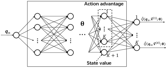
With the above action space discretization, the action-value function contains the continuous state input and the discrete action input . We use the state-of-the-art DQN with the dueling network architecture [16] to approximate , as illustrated in Fig. 3. At each time step , the input of the network corresponds to the state (or the UAV location) , and it has outputs, each corresponding to one action in . Note that the distinguishing feature of dueling DQN is to first separately estimate the state values and the state-dependent action advantages, and then combine them in a smart way via an aggregating layer to give an estimate of the action value function Q [16]. Compared to the standard DQN, dueling DQN is able to learn the state-value function more efficiently, and is also more robust to the approximation errors when the action-value gaps between different actions of the same state are small [16]. The coefficients of the dueling DQN are denoted as , which is trained so that the output gives good approximations to the true action-value function .
To train the dueling DQN, besides the standard techniques of experience replay and target network as discussed in Section III-B, we also apply the multi-step DDQN learning techniques [38]. Specifically, define the truncated -step return from a given state as
| (31) |
Then a multi-step DQN learning is to minimize the loss given by [14]
| (32) |
It is known that multi-step learning with appropriately chosen usually leads to faster learning [14].
Furthermore, double Q learning has been widely used to address the overestimation bias of the maximum operation in (32), via using two separate networks for the action selection and value evaluation of bootstrapping. Specifically, with DDQN, the loss of the multi-step learning in (32) is changed to
| (33) |
where
| (34) |
Note that we have used the target network with coefficients to evaluate the bootstraping action in (33) while using the Q network with coefficients for action selection in (34).
The proposed algorithm for coverage-aware UAV navigation with dueling DDQN multi-step learning is summarized in Algorithm 1. Note that the main steps of Algorithm 1 follow from the classic DQN algorithms in [15], except the following modifications. First, the more advanced dueling DQN architecture is used, instead of DQN. Second, to enable multi-step learning, a sliding window queue with capacity as in steps 6 and 11 is used to store the latest transitions. Therefore, at the current time step , the UAV can calculate the accumulated return from the previous time steps, as in step 12 of Algorithm 1. Third, a double DQN learning is used in step 14.
While theoretically, the convergence of Algorithm 1 is guaranteed [14], in practice, a random initialization of the dueling DQN may require a prohibitively large number of time steps for the UAV to reach the destination . Intuitively, should be initialized in a way such that in the early episodes when the UAV has no or limited knowledge about the radio environment, it should be encouraged to select actions for the shortest path flying. Thus, we propose the distance-based initialization for Algorithm 1, with initialized so that approximates , where is the next state with current state and action . Note that as the distance from any location to the destination is known a priori, the above initialization can be performed by sampling some locations in without requiring any interaction with the environment. With such an initialization, it can be obtained from step 9 of Algorithm 1 that the UAV will choose the shortest-path action in the first episode with probability , and random exploration with probability . As the UAV accumulates more experience after some episodes so that the dueling DQN has been substantially updated, the -greedy policy in step 9 would generate UAV flying path that achieves a balance between minimizing the flying distance and avoiding the weak coverage region, as desired for problem .
IV-C Simultaneous Navigation and Radio Mapping
The dueling DDQN multi-step learning proposed in Algorithm 1 is a model-free Q learning algorithm, where all data used to update the estimation of the action-value function is obtained via the direct interaction of the UAV with the environment, as in step 10 of Algorithm 1. While model-free RL requires no prior knowledge about the environment nor intending to estimate it, it usually leads to slow learning process and requires a large number of agent-environment interactions, which is typically costly or even risky to obtain. For instance, for the coverage-aware UAV navigation problem considered in this paper, each step 10 in Algorithm 1 actually requires to fly the UAV and perform signal measurements at designated locations to get the empirical outage probability so as to obtain the reward value. Extensive UAV flying increases the safety risk due to e.g., mechanical fatigue. To overcome the above issues, in this subsection, we propose a novel SNARM framework for cellular-connected UAVs by utilizing the dueling DDQN multi-step learning algorithm with model learning [14].
For RL with model learning, each real experience obtained by the UAV-environment interaction can actually be used for at least two purposes: for direct RL as in Algorithm 1 and for model learning so as to gain useful information about the environment. A closer look at the MDP corresponding to problem would reveal that the essential information needed for coverage-aware navigation is the reward function , which depends on the outage probability for any location visited by the UAV. Therefore, model learning for corresponds to learning the radio map of the airspace where the UAVs are operating, which specifies the cellular outage probability , . Thus, the actual measurement of the outage probability at location can be simultaneously used for navigation, i.e., determining the UAV flying direction for the next time step, and also for radio mapping, i.e., helping to predict the outage probability for locations that the UAV has not visited yet. This leads to our proposed framework of SNARM.
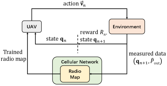
A high-level overview of SNARM is illustrated in Fig. 4. Different from the standard RL setup, with SNARM for cellular-connected UAV, the cellular network (say, a selected macro-cell in the area of interest) maintains a radio map containing an estimation of the cellular outage probability for all locations in . Note that might be highly inaccurate initially, but can be continuously improved as more real experience is accumulated. For any cellular-connected UAV flying in the considered airspace , it may either download the radio map from the network off-line before the mission starts, or continuously receive the latest update of in real time. At each time step as the UAV performs its mission, it observes its current location , together with the radio map , then determines its flying direction for the next step. After executing the action and reaching the new location , it measures the empirical outage probability , and receives the corresponding reward . The obtained empirical outage probability based on signal measurement can be used as the new data input to improve the radio map estimation. In the following, we explain the radio map update and UAV action selection of SNARM, respectively.
With any finite measurements , predicting the outage probability is essentially a supervised learning problem. In this paper, we use a feedforward fully-connected ANN with parameters to represent the radio map, i.e., is trained so that , . Note that compared to the standard supervised learning problem, the radio mapping problem has two distinct characteristics. First, the data measurement only arrives incrementally as the UAV flies to new locations, instead of all made available at the beginning of the training. Second, as the UAV performs signal measurements as it flies, those data obtained at consecutive time steps are typically correlated, which is undesirable for supervised training. To tackle these two issues, similar to Algorithm 1, we use a database (replay memory) to store the measured data , and at each training step, a minibatch is sampled at random from the database to update the network parameter .
On the other hand, the problem for UAV action selection with the assistance of a radio map is known as indirect RL, for which various algorithms have been proposed [14]. Different from that for direct RL in Algorithm 1, with the radio map in SNARM, the UAV is able to predict the estimated return for each trajectory it would take, without having to actually fly along it. As a result, we may generate as much simulated experience as we wish based on , which, together with the real experience, can be used to update the UAV policy based on any RL algorithm, such as Algorithm 1. However, as the radio map might be inaccurate at the initial stages, over-relying on the simulated experience may result in poor performance due to the model error. Therefore, we need to seamlessly integrate the learning with simulated experience based on the radio map and that with the real experience. A simple but effective architecture achieving this goal is known as Dyna [14], where for each RL update based on the real experience, we have several updates based on the simulated experience. The proposed SNARM based on Dyna dueling DDQN with multi-step learning is summarized in Algorithm 2.
Obviously, Algorithm 2 expands Algorithm 1 by inserting the radio map learning operations and the double DQN update based on simulated UAV experience. Note that the simulated trajectory is initialized independently from the real trajectory (see steps 3 and 12 of Algorithm 2), and it is used times more frequently than the real trajectory, i.e., for each actual step the UAV takes in real experience, steps will be taken in the simulated trajectory, as in steps 7 to 13. Note that in general, should be increasing with the number of episodes, since as more real experience is accumulated, the constructed radio map becomes more accurate, which makes the predicted returns of the simulated trajectories more reliable. Regardless of simulated or real experience, the same action-value update based on dueling DDQN multi-step learning is performed. Besides, the radio map is updated in step 6 based on the actual measurement data, and used in step 9 to generate simulated UAV experience.
V Numerical Results
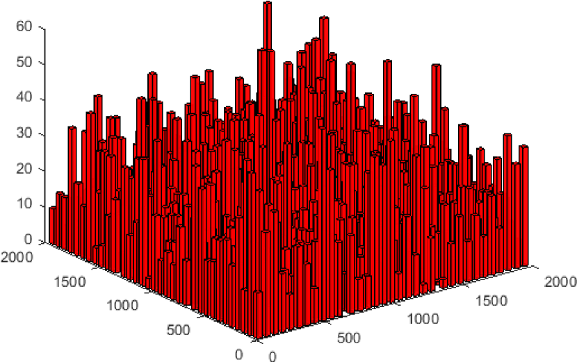
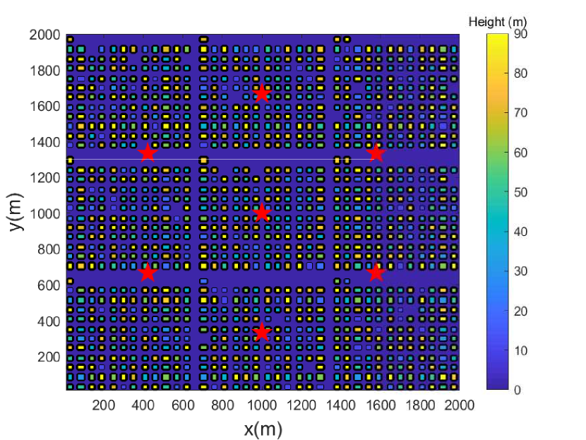
In this section, numerical results are provided to evaluate the performance of the proposed algorithms. As shown in Fig. 5, we consider an urban area of size 2 km 2 km with high-rise buildings, which corresponds to the most challenging environment for coverage-aware UAV navigation, since the LoS/NLoS links and the received signal strength may alter frequently as the UAV flies (see Fig. 1). To accurately simulate the BS-UAV channels in the given environment, we first generate the building locations and heights based on one realization of the statistical model suggested by International Telecommunication Union (ITU) [40], which involves three parameters, namely, : the ratio of land area covered by buildings to the total land area; : the mean number of buildings per unit area; and : a variable determining the building height distribution, which is modelled as Rayleigh distribution with mean value . Note that such statistical building model has been widely used to obtain the LoS probability for aerial-ground links [11], which, however, only reflects the average characteristics over a large number of geographic areas of similar type. While for each local area with given building locations and heights, the presence/absence of LoS links with cellular BSs can be exactly determined by checking whether the line connecting the BS and UAV is blocked or not by any building. Fig. 5 shows the 3D and 2D views of one particular realization of the building locations and heights with , buildings/km2, and m. For convenience, the building height is clipped to not exceed m.
We assume that the considered area has 7 cellular BS sites with locations marked by red stars in Fig. 5, and the BS antenna height is m [7]. With the standard sectorization technique, each BS site contains 3 sectors/cells. Thus, the total number of cells is . The BS antenna model follows the 3GPP specification [5], where an 8-element uniform linear array (ULA) is placed vertically. Each array element itself is directional, with half-power beamwidths along the vertical and horizontal dimensions both equal to . Furthermore, pre-determined phase shifts are applied to the vertical antenna array so that its main lobe is electrically downtilted towards the ground by . This leads to the directional antenna array with fixed 3D radiation pattern, as shown in Fig. 4 of [2]. To simulate the signal strength received by the UAV from each cell, we firstly determine whether there exists an LoS link between the UAV and each BS at the given UAV location based on the building realization, and then generate the BS-UAV path loss using the 3GPP model for urban Macro (UMa) given in Table B-2 of [7]. The small-scale fading coefficient is then added assuming Rayleigh fading for the NLoS case and Rician fading with 15 dB Rician factor for the LoS case. It is worth mentioning that for a given environment, the aforementioned LoS condition, antenna gain, path loss and small-scale fading with each BS are all dependent on the UAV location in a rather sophisticated manner. This makes them only suitable to generate the numerical values with given UAV location, instead of being directly used for UAV path planning with the conventional optimization technique as for solving , even with accurate channel modelling and perfect global information. This thus justifies the use of RL techniques for UAV path design as pursued in this paper.
For both Algorithms 1 and 2, the dueling DQN adopted is a fully connected feedforward ANN consisting of 5 hidden layers. The numbers of neurons of the first 4 hidden layers are 512, 256, 128, and 128, respectively. The last hidden layer is the dueling layer with neurons, with one neuron corresponding to the estimation of the state-value and the other neurons corresponding to the action advantages for the actions, i.e., the difference between the action values and the state value of each state. The outputs of these neurons are then aggregated in the output layer to obtain the estimation of the action values [16], as shown in Fig. 3. For SNARM in Algorithm 2, the ANN for radio mapping also has 5 hidden layers, with the corresponding numbers of neurons given by 512, 256, 128, 64, and 32, respectively. The activation for all hidden layers is by ReLu [37], and the ANN is trained with Adam optimizer to minimize the mean square error (MSE) loss, using Python with TensorFlow and Keras.333https://keras.io/ For ease of illustration, we assume that the UAV’s flying altitude is fixed as m, and the number of actions (or flying directions) at each time step is . All UAV missions have a common destination location m, while their initial locations are randomly generated. The transmit power of each cell is assumed to be dBm and the outage SIR threshold is dB. Other major simulation parameters are summarized in Table I.
| Simulation parameter | Value |
|---|---|
| Maximum number of episodes | 5000 |
| Initial exploration parameter | 0.5 |
| Exploration decaying rate | 0.998 |
| Replay memory capacity | 100000 |
| Steps for multi-step learning | 30 |
| Update frequency for target network | 5 |
| Maximum step per episode | 200 |
| Step displacement | 10 m |
| Reaching-destination reward | 200 |
| Outbound penalty | 10000 |
| Outage penalty weight | 40 |
| Number of signal measurements per time step | 1000 |
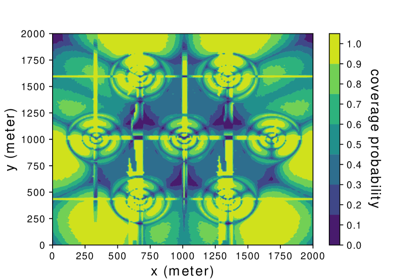
Fig. 6(a) shows the true global coverage map for the considered area, i.e., the coverage (non-outage) probability for each location by the cellular network, where coverage probability is the complementary probability of the outage probability defined in (6). Note that such a global coverage map is numerically obtained based on the aforementioned 3D building and channel realizations via computer simulations, while it is not available for our proposed Algorithm 1 or Algorithm 2. It is observed from Fig. 6(a) that the coverage pattern in the sky is rather irregular due to the joint effects of the 3D BS antenna radiation pattern and building blockage. It is observed that around the center of the area, there are several weak coverage regions with coverage probability less than . Obviously, effective coverage-aware UAV navigation should direct UAVs to avoid entering such weak coverage regions with the best effort.
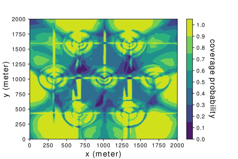
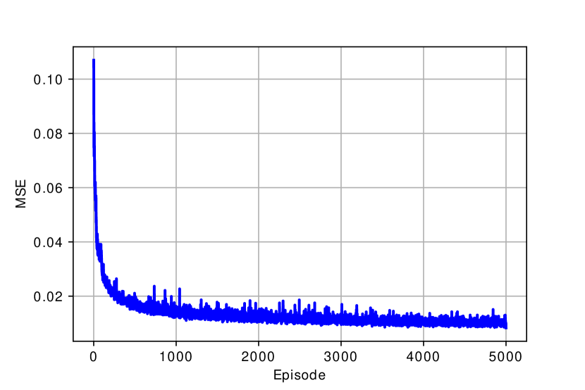
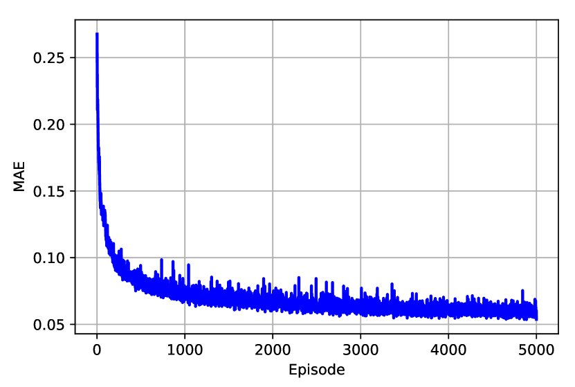
To validate the quality of radio map estimated by the SNARM framework proposed in Algorithm 2, Fig. 6(b) shows the finally learned coverage map by Algorithm 2. By comparing Fig. 6(a) and Fig. 6(b), it is observed that the learned coverage map is almost identical to the true map, with only slight differences. This thus validates the effectiveness of applying SNARM for the radio map estimation and coverage-aware path learning based on it. This is further corroborated by Fig.7, which shows the MSE and mean absolute error (MAE) of the learned radio map versus the episode number. Note that the MSE and MAE are calculated by comparing the predicted outage probabilities using the learned radio map versus their actual values in the true map for a set of randomly selected locations. It is observed that the quality of the learned radio map is rather poor initially, but it improves rather quickly with the episode number as more signal measurements are accumulated. For example, with only 200 episodes, we can already achieve 87.1% of the MSE reduction that is achieved after 5000 episodes.
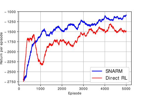
As for the performance of the proposed learning algorithms, Fig. 8 shows the moving average return per episode for the direct RL in Algorithm 1 and SNARM in Algorithm 2, where the moving window has the length of 200 episodes. For the SNARM algorithm, the number of steps based on simulated experience per actual step at episode is set as , so that increases with the episode number and converges to 10. Recall that the return of each episode for RL is the accumulated rewards for all time steps in the episode. It is observed that though experiencing certain fluctuation, as usually the case for RL algorithms, both proposed algorithms demonstrate an overall tendency of increasing average return. Furthermore, recall that the dueling DQNs are initialized to encourage shortest path flying for the early episodes when the UAV has completely no knowledge about the radio environment, which leads to an average return about initially. After training for 5000 episodes, the resulting return has increased to and for SNARM and direct RL, respectively. Another observation from the figure is that the direct RL has faster improvement over the SNARM algorithm at the earlier episodes. This is probably due to the insufficient accuracy of the learned radio map for SNARM, which may generate inefficient simulated experience. However, as the quality of the radio map improves, the SNARM algorithm achieves better performance than direct RL, thanks to its exploitation of the learned radio map for path planning. In practice, such a performance improvement translates to fewer agent-environment interactions, which is highly desirable due to the usually high cost of data acquisition from real experience. For example, to achieve an average return of , Fig. 8 shows that about 3200 actual UAV flight episodes are required for direct RL in Algorithm 1, but this number is significantly reduced to about 1000 with SNARM in Algorithm 2.
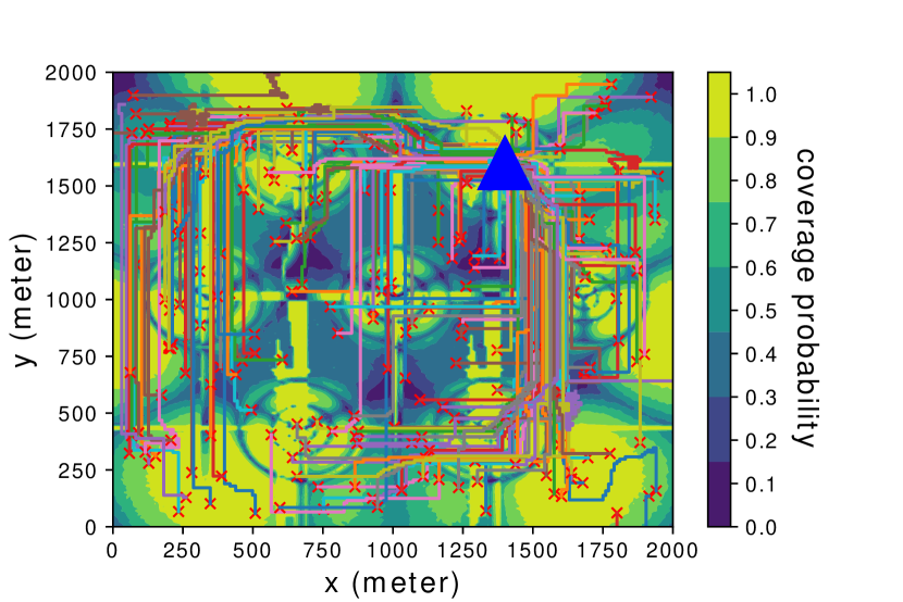
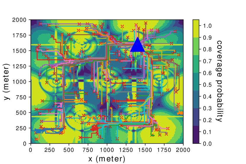
Last, Fig. 9 shows the resulting UAV paths with the proposed algorithms for the last 200 episodes of learning, which correspond to 200 randomly generated initial locations, as denoted by red crosses in the figure. The common destination location is labelled by a big blue triangle. Also shown in the figure is the true global coverage map. It is observed that both direct RL and SNARM algorithms are able to direct the UAVs to avoid the weak cellular coverage regions with the best effort, as evident from the generally detoured UAV paths as well as the much sparser paths in areas with low coverage probabilities. For example, as can be seen from Fig. 9(b), the SNARM algorithm is able to discover and follow the narrow “radio bridge” located at the x axis around 1000 m and the y axis from about 1000 m to 1700 m. This shows the peculiar effectiveness of SNARM for coverage-aware UAV path learning.
VI Conclusions
This paper studies coverage-aware navigation for cellular-connected UAVs. To overcome the practical limitations of the conventional optimization-based path design approaches, we propose DRL-based algorithms, which only require UAV signal measurements as the input. By utilizing the state-of-the-art dueling DDQN with multi-step learning, a direct RL-based algorithm is first proposed, followed by the more advanced SNARM framework to enable radio mapping and reduce the real UAV flights for data acquisition. Numerical results are provided to show the effectiveness of the proposed algorithms for coverage-aware UAV navigation, and the superior performance of SNARM over direct RL based navigation.
References
- [1] Y. Zeng and X. Xu, “Path design for cellular-connected UAV with reinforcement learning,” in Proc. IEEE Global Communications Conference (GLOBECOM), 2019.
- [2] Y. Zeng, Q. Wu, and R. Zhang, “Accessing from the sky: a tutorial on UAV communications for 5G and beyond,” Proc. of the IEEE, vol. 107, no. 12, pp. 2327–2375, Dec. 2019.
- [3] Y. Zeng, R. Zhang, and T. J. Lim, “Wireless communications with unmanned aerial vehicles: opportunities and challenges,” IEEE Commun. Mag., vol. 54, no. 5, pp. 36–42, May 2016.
- [4] Y. Zeng, J. Lyu, and R. Zhang, “Cellular-connected UAV: potentials, challenges and promising technologies,” IEEE Wireless Commun., vol. 26, no. 1, pp. 120–127, Feb. 2019.
- [5] 3GPP TR 36.873: “Study on 3D channel model for LTE”, V12.7.0, Dec., 2017.
- [6] Qualcomm, “LTE unmanned aircraft systems,” trial Report, available online at https://www.qualcomm.com/documents/lte-unmanned-aircraft-systems-trial-report, May, 2017.
- [7] 3GPP TR 36.777: “Technical specification group radio access network: study on enhanced LTE support for aerial vehicles”, V15.0.0, Dec., 2017.
- [8] S. Zhang, Y. Zeng, and R. Zhang, “Cellular-enabled UAV communication: a connectivity-constrained trajectory optimization perspective,” IEEE Trans. Commun., vol. 67, no. 3, pp. 2580–2604, Mar. 2019.
- [9] S. Zhang and R. Zhang, “Trajectory design for cellular-connected UAV under outage duration constraint,” in Proc. IEEE Int. Conf. Commun. (ICC), May, 2019.
- [10] E. Bulut and I. Guvenc, “Trajectory optimization for cellular-connected UAVs with disconnectivity constraint,” in Proc. IEEE International Conference on Communications (ICC), May 2018.
- [11] A. Al-Hourani, S. Kandeepan, and S. Lardner, “Optimal LAP altitude for maximum coverage,” IEEE Wireless Commun. Lett., vol. 3, no. 6, pp. 569–572, Dec. 2014.
- [12] M. M. Azari, F. Rosas, K.-C. Chen, and S. Pollin, “Ultra reliable UAV communication using altitude and cooperation diversity,” IEEE Trans. Commun., vol. 66, no. 1, pp. 330–344, Jan. 2018.
- [13] C. You and R. Zhang, “3D trajectory optimization in Rician fading for UAV-enabled data harvesting,” IEEE Trans. Wireless Commun., vol. 18, no. 6, pp. 3192–3207, Jun. 2019.
- [14] R. S. Sutton and A. G. Barto, Reinforcement learning: An introduction, 2nd ed. MIT Press, Cambridge, MA, 2018.
- [15] V. Mnih, et al., “Human-level control through deep reinforcement learning,” Nature, vol. 518, pp. 529–533, Feb. 2015.
- [16] Z. Wang, et al., “Dueling network architectures for deep reinforcement learning,” in Proc. of the 33rd Int. Conf. Machine Learning, Jun. 2016, pp. 1995–2003.
- [17] J. Chen, U. Yatnalli, and D. Gesbert, “Learning radio maps for UAV-aided wireless networks: a segmented regression approach,” in Proc. IEEE International Conference on Communications (ICC), May 2017.
- [18] S. Bi, J. Lyu, Z. Ding, and R. Zhang, “Engineering radio map for wireless resource management,” IEEE Wireless Commun., vol. 26, no. 2, pp. 133–141, Apr. 2019.
- [19] H. Bayerlein, P. Kerret, and D. Gesbert, “Trajectory optimization for autonomous flying base station via reinforcement learning,” in Proc. IEEE SPAWC, Jun. 2018.
- [20] L. Xiao, X. Lu, D. Xu, Y. Tang, L. Wang, and W. Zhuang, “UAV relay in VANETs against smart jamming with reinforcement learning,” IEEE Trans. Veh. Technol., vol. 67, no. 5, pp. 4087–4097, May 2018.
- [21] J. Cui, Y. Liu, and A. Nallanathan, “Multi-agent reinforcement learning based resource allocation for UAV networks,” IEEE Trans. Wireless Commun., Aug. 2019, early Access.
- [22] B. Khamidehi and E. S. Sousa, “Reinforcement learning-based trajectory design for the aerial base stations,” available online at https://arxiv.org/pdf/1906.09550.pdf.
- [23] J. Hu, H. Zhang, and L. Song, “Reinforcement learning for decentralized trajectory design in cellular UAV networks with sense-and-send protocol,” IEEE Internet of Things Journal, vol. 6, no. 4, pp. 6177–6189, Aug. 2019.
- [24] N. C. Luong, et al., “Applications of deep reinforcement learning in communications and networking: a survey,” IEEE Commun. Surveys Tuts., vol. 21, no. 4, pp. 3133–3174, Fourthquarter 2019.
- [25] Y. Yu, T. Wang, and S. C. Liew, “Deep-reinforcement learning multiple access for heterogeneous wireless networks,” IEEE J. Selected Areas Commun., vol. 37, no. 6, pp. 1277–1290, Jun. 2019.
- [26] Y. S. Nasir and D. Guo, “Multi-agent deep reinforcement learning for dynamic power allocation in wireless networks,” IEEE J. Selected Areas Commun., vol. 37, pp. 2239–2250, 2019.
- [27] L. Zhang, J. Tan, Y.-C. Liang, G. Feng, and D. Niyato, “Deep reinforcement learning based modulation and coding scheme selection in cognitive heterogeneous networks,” IEEE Trans. Wireless Commun., vol. 18, no. 6, pp. 3281–3294, Jun. 2019.
- [28] L. Huang, S. Bi, and Y. J. Zhang, “Deep reinforcement learning for online computation offloading in wireless powered mobile-edge computing networks,” IEEE Trans. Mobile Computing, Jul. 2019, early access.
- [29] J. Qiu, J. Lyu, and L. Fu, “Placement optimization of aerial base stations with deep reinforcement learning,” available online at https://arxiv.org/abs/1911.08111.
- [30] U. Challita, W. Saad, and C. Bettstetter, “Interference management for cellular-connected UAVs: a deep reinforcement learning approach,” IEEE Trans. Wireless Commun., vol. 18, no. 4, pp. 2125–2140, Apr. 2019.
- [31] S. Zhang and R. Zhang, “Radio map based path planning for cellular-connected UAV,” in Proc. IEEE Global Communications Conference (GLOBECOM), Dec. 2019.
- [32] J. Chen and D. Gesbert, “Local map-assisted positioning for flying wireless relays,” arXiv:1801.03595, 2018.
- [33] O. Esrafilian, R. Gangula, and D. Gesbert, “3D-map assisted uav trajectory design under cellular connectivity constraints,” available online at https://arxiv.org/abs/1911.01124.
- [34] C. You and R. Zhang, “Hybrid offline-online design for UAV-enabled data harvesting in probabilistic LoS channel,” available online at https://arxiv.org/abs/1907.06181.
- [35] X. Xu and Y. Zeng, “Cellular-connected UAV: performance analysis with 3D antenna modelling,” in Proc. IEEE International Conference on Communications (ICC) Workshops, May 2019.
- [36] M. Hessel, et al., “Rainbow: Combining improvements in deep reinforcement learning,” in Proc. of AAAI, 2018.
- [37] I. Goodfellow, Y. Bengio, and A. Courville, Deep Learning. MIT Press, 2016, http://www.deeplearningbook.org.
- [38] H. Hasselt, A. Guez, and D. Silver, “Deep reinforcement learning with double Q-learning,” in Proc. of AAAI, 2016, pp. 2094–2100.
- [39] T. Schaul, J. Quan, I. Antonoglou, and D. Silver, “Prioritized experience replay,” in Proc. of ICLR, 2015.
- [40] ITU-R, Rec. P.1410-5 “Propagation data and prediction methods required for the design of terrestrial broadband radio access systems operating in a frequency range from 3 to 60 GHz”, Radiowave propagation, Feb. 2012.