Simultaneous Modeling of Disease Screening and Severity Prediction: A Multi-task and Sparse Regularization Approach
Abstract
The exploration of biomarkers, which are clinically useful biomolecules, and the development of prediction models using them are important problems in biomedical research. Biomarkers are widely used for disease screening, and some are related not only to the presence or absence of a disease but also to its severity. These biomarkers can be useful for prioritization of treatment and clinical decision-making. Considering a model helpful for both disease screening and severity prediction, this paper focuses on regression modeling for an ordinal response equipped with a hierarchical structure. If the response variable is a combination of the presence of disease and severity such as {healthy, mild, intermediate, severe}, for example, the simplest method would be to apply the conventional ordinal regression model. However, the conventional model has flexibility issues and may not be suitable for the problems addressed in this paper, where the levels of the response variable might be heterogeneous. Therefore, this paper proposes a model assuming screening and severity prediction as different tasks, and an estimation method based on structural sparse regularization that leverages any common structure between the tasks when such commonality exists. In numerical experiments, the proposed method demonstrated stable performance across many scenarios compared to existing ordinal regression methods.
1 Introduction
One of the important issues in biomedical research is the exploration of biomarkers and the construction of clinical prediction models. Biomarkers are physiological indicators or biomolecules used for various purposes such as disease screening, prognosis, and estimation of treatment effects, and they are widely used in clinical practice (Biomarkers Definitions Working Group., 2001). This paper focuses specifically on biomarkers used for disease screening, aiming to propose models and estimation methods for the exploration of biomarkers that are not only useful for screening but can also predict the disease severity at screening. First, we will show examples of such muti-purpose biomarkers.
Alpha-fetoprotein (AFP), Des-gamma-carboxyprothrombin, and Lens culinaris agglutinin-reactive fraction of AFP are well-known biomarkers for hepatocellular carcinoma. These biomarkers are measured through blood testing and serve as less invasive diagnostic markers for HCC. Furthermore, it has been reported that these markers are associated with prognosis and cancer stage (Omata et al., 2017; for the Study of the Liver, 2018). Another example is neuroblastoma, which is a type of childhood cancer known to have a wide range of severity (Irwin et al., 2021). It is known that neuroblastoma patients excrete specific metabolites in their urine, and conventionally, molecules such as homovanillic acid (HVA) and vanillylmandelic acid (VMA) have been used for disease screening. However, while these are highly effective in screening neuroblastoma, their association with severity is weak. Recently, a metabolomics study has revealed some markers are useful for screening and related to severity, beyond HVA and VMA (Amano et al., 2024).
How should we take into account disease screening and severity prediction at one time? A simple way would be to stack them into one ordinal variable. In other words, to define the absence of disease as the lowest category and set higher categories for increasing disease severity, treating it as an ordinal categorical variable. In regression analysis, an ordinal categorical variable is one of the most common types of response variables. A well-known regression model for ordinal responses is the cumulative logit model (CLM, a.k.a. the proportional odds model; McCullagh, 1980). CLM assumes a continuous latent variable behind the response variable, and the response variable level increases when the latent variable exceeds certain thresholds. CLM is also widely used in biomedical studies (e.g., Muchie, 2016; Jani et al., 2017). However, this approach may have an issue applying to our problem; CLM assumes an identical relationship between the response and the predictor across all levels of the response variable, which is referred to as parallelism assumption. The parallelism assumption is questionable for the combined response because the two tasks, screening and severity prediction, do not necessarily share the same structure; in other words, the same predictors do not necessarily contribute in the same way to screening and severity prediction. One possible solution to this issue is to relax the parallelism assumption using a varying coefficient version of CLM, which we call non-parallel CLM (NPCLM). However, as discussed in Section 2, the varying coefficient approach could make the estimation and interpretation of the model difficult.
To address the problem of modeling the combined task, we propose a model incorporating the idea of multi-task learning, we aim to effectively construct a prediction model and discover beneficial biomarkers, even in high-dimensional settings. Multi-task learning is a machine learning approach where multiple models are trained simultaneously, leveraging shared information and structures across the tasks to improve predictive performance (Caruana, 1997). Multi-task learning is applied in many fields such as computer vision, natural language processing, and web applications (Zhang and Yang, 2017). Furthermore, multi-task learning is being incorporated in the area of biomarker discovery. For example, Wang et al. (2020) introduced multitask learning to identify genes expressed across multiple types of cancer. While there are not many examples of applying multi-task learning to ordinal regression, Xiao et al. (2023), for instance, deals with multi-task learning for parallel ordinal regression problems.
This paper is organized as follows. In Section 2, we review CLM, NPCLM, and related extensions. In Section 3, we propose a novel prediction model and also discuss its relationships with other categorical models and potential extensions. In Section 4, we introduce an estimation method using sparse regularization and an optimization algorithm. The proposed models employ structural sparse penalties to exploit the common structure between screening and severity prediction. In Section 5, we present the results of simulation experiments, considering various structures between screening and severity prediction, and clarifying under what conditions the proposed method performs well. In Section 6, we report the results of real data analysis. Finally, we make some concluding discussion in Section 7.
2 Cumulative Logit Model
For ordinal responses, CLM is one of the most popular regression models (McCullagh, 1980; Agresti, 2010). Let
the response and the predictors, where is the -dimensional predictor space, and the set is equipped with an ordinal relation of natural numbers. CLM is defined as
where and are the intercepts and regression coefficients, and . CLM has an important interpretation. Suppose that there is a latent continuous variable behind the response and that is associated with the predictors as
where is the regression parameters for , and is the standard logistic distribution. Then, by defining with an increasing sequence with and , we have
where is the cumulative distribution function of . By replacing for all and , we can see that this model is equivalent to CLM. Therefore, we can see as the thresholds determining the class based on the latent variable . The linear functions representing the log-odds of the cumulative probability of each level are all parallel because they share the same slope . The parallelism assumption is necessary to ensure that the model is valid in the sense that the conditional cumulative probability derived from CLM is monotonic at any given (e.g., Okuno and Harada (2024)).
The non-parallel CLM (NPCLM), sometimes called the non-proportional odds model, is the model with different slopes for each response level. This implies the conditional cumulative probability curves of NPCLM can be non-monotone. Such curves violate the appropriate ordering of the response probabilities. So NPCLM is more flexible and expressive than CLM, but it is valid on some restricted subspace of . Peterson et al. (1990) proposed a model that is intermediate between CLM and NPCLM (Peterson and Harrell, 1990). This partial proportional odds model is defined as follows:
| (1) |
where is the variable slope of the th level. This model is designed to capture the homogeneous effect by and the heterogeneous effect by . Still, similarly to NPCLM, this model is generally valid as a probability model only on the restricted subspace of . To control the balance of flexibility and monotonicity, various estimation techniques with regularization have been proposed. Wurm et al. (2021) use L1 and/or L2 norm on coefficient parameters and of the partial proportional odds model (Wurm et al., 2021). If the parallel assumption holds, then should be zero due to L1 penalization, and even when the parallel assumption is violated, the variability of is controlled by the penalties. Wurm et al. (2021) have also proposed an efficient coordinate descent algorithm (Wurm et al., 2021), which is similar to that of the lasso regression (Tibshirani, 1996; Hastie et al., 2015). Tutz et al. (2016) have introduced the penalization on the difference of the adjacent regression coefficient (Tutz and Gertheiss, 2016). For NPCLM, their penalty term is , resulting in smoothed coefficients between the adjacent response levels. They use the L1 penalty for the adjacent coefficients instead of the L2 penalty. With the L1 penalty, unlike the L2 penalty, the adjacent regression coefficients are expected to be estimated as the same if the parallelism assumption holds. Additionally, they have proposed an algorithm based on the Alternating Direction Method of Multipliers (ADMM; Boyd et al. (2011)).
In our setting, the non-parallel models may be helpful, but as previously discussed, they can be non-monotone for given . Furthermore, although these models are linear, they are sometimes not easy to interpret. If the estimated coefficients indicate that and have different coefficients with opposite sign for , it may be difficult to understand, given that the event includes . In the next section, we propose a multi-task learning approach that maintains monotonicity over the entire and possesses a flexibility that allows it to capture the different structures between the tasks of screening and severity prediction.
3 Proposed Model
3.1 Definition and interpretation
Let be an ordinal outcome for which zero indicates the case being healthy, and corresponds to disease severity. Our model, which we call Multi-task Cumulative Linear Model (MtCLM), is defined as
| (2) | ||||
| (3) |
where are model parameters. We refer to model (2) as the screening model and model (3) as the severity model. The screening model is a simple logistic regression model, while the severity model defines CLM for severity within the patient group. Note that the parameters are assumed to be variationally independent, meaning an estimator that maximizes the joint likelihood of (2) and (3) is equivalent to an estimator that maximizes the likelihood of (2) and (3) separately. When estimated using the penalized maximum likelihood method introduced in the next section, the proposed model can exploit the shared structure between screening and severity prediction.
Similarly to CLM, the proposed model has a latent-variable interpretation. Let be the latent random variables, and define as follows:
where is a thresholding parameter, is an increasing sequence in which and , are regression coefficients, and are independent errors drawn from the standard logistic distribution. Then, we obtain
That is, the proposed model supposes that there are latent variables behind screening and severity prediction and that they share the association structure through . As noted above, we leverage the shared structure between screening and severity prediction by penalized likelihood-based estimation.
It should be noted that MtCLM is not restricted to its current form, specifically, the combination of screening and severity prediction. Indeed, it could be reworked into a more comprehensive framework. For instance, we are not limited to binary screening for the first-level model, or we can set a deeper hierarchy. More flexible models, such as a multinomial logit model, can also be incorporated. Despite the potential generalizability, we choose to use the current form of MtCLM for two reasons. Firstly, a more generalized version could potentially increase complexity, making interpretation and practical application more challenging. Secondly, our aim in this paper is to propose a method that captures the shared structural predictors in screening and severity prediction, so more flexible models are beyond our scope.
3.2 Relationships to other categorical and ordinal models
Our model is related to other models with ordinal or non-ordinal categorical regression models. Let and . Then, the conditional cumulative probability for is
where is a sigmoid function: i.e., the inverse of function. We can see if , which means , the MtCLM reduces to CLM for . Also, we can see that MtCLM is non-parallel even if because the gradient with respect to depends on . The relationship between CLM and MtCLM is not straightforward due to the non-linearity of the sigmoid and logit functions.
We can see that the multinomial logit model (MLM) has a more clear relationship with MtCLM than CLM. Let , where is the linear predictor for the th level. Then, we obtain the following expression of the conditional probability of MtCLM:
| (4) | ||||
| (5) |
There are many other regression models for an ordinal response (Agresti, 2010). The continuation ratio logit model assumes that the conditional probability is logit-linear for all s, meaning that MtCLM is locally equivalent to the continuation ratio logit model at . The adjacent category logit model expresses the logarithm of as a linear function. These models are flexible and do not violate the monotonicity of the cumulative probabilities. They are also useful and may be a good choice when there is a need for more flexible models. Specifically, if it is assumed that the variables important for lower and higher levels of severity prediction differ, these models could be quite useful. The partitioned conditional model (PCM; Zhang and Ip, 2012) is a regression model for a broad class of categorical responses with hierarchical structures. It is introduced to model partially ordered response, where some of their categories have ordinal relationships. This model encompasses MLM, CLM, and MtCLM as special cases. If more complex structures need to be modeled, it might be beneficial to refer to more general models like the PCMs. However, it is important to note that as the hierarchical structure becomes more complex, the devices for capturing shared structures among tasks can become more intricate.
As we see in Section 6, there is sometimes an insufficient number of cases at some levels of severity prediction. One reason that MtCLM imposes a monotonicity assumption on the severity prediction model is to conduct stable estimation even in such situations. Besides, the interpretation of the odds ratios varies model by model: the continuation ratio logit model estimates, for example, the odds ratio of intermediate to more than intermediate among the patients with of intermediate or severe. The adjacent category logit model does not take into account the severe patients or healthy individuals when discussing mild vs. intermediate since it estimates the odds ratios of pairwise comparisons for adjacent categories. In contrast, MtCLM can be interpreted in the same way as a conventional logistic regression model for the screening model and as a conventional CLM for the severity prediction model. Although the final choice of model depends on the research purpose, MtCLM’s strength also lies in its small deviation from the popular models.
4 Sparse Estimation and Algorithm
As noted in Section 3, we cannot exploit the shared structure of the two tasks, screening and severity prediction, through simple maximum likelihood estimation. Therefore, we employ a penalized maximum likelihood approach.
4.1 Penalized Likelihood for MtCLM
The log-likelihood of MtCLM is given by
| (6) |
Here,
| (7) | ||||
| (8) |
where , , and . Since we let and , and for all . The log-likelihood for MtCLM is a sum of the log-likelihoods of the logistic regression model for screening and the CLM for severity prediction.
If the two probablilities, and have the similar associations with the feature , the corresponding regression coefficients and are supposed to be similar. We implement this intuition using two types of structural sparse penalty terms, namely, the fused lasso-type penalty (Tibshirani et al., 2005) and the group lasso-type penalty (Yuan and Lin, 2006). These two types of penalty terms are defined as follows:
| (9) | |||
| (10) |
where are tuning parameters determining the intensity of regularization.
The estimator of MtCLM is defined as the minimizer of the penalized log-likelihoods:
| (11) | |||
| (12) |
where are tuning parameters for L1 penalties of and . We can enhance sparsity of and by setting to be nonzero. It would be possible to incorporate both and simultaneously, but we discuss them separately because they exploit the shared structure of the screening and severity prediction models in different ways.
In general, sparse regularization problems can be viewed as optimization problems under inequality constraints (Hastie et al., 2015). Figure 1 illustrates the optimization problems with inequality constraints for both the fused lasso type and the group lasso type, and it intuitively explains how the solutions to these problems would be obtained. The group lasso-type regularization uniformly selects when it is related to , regardless of the positions of the true point , and a uniform bias toward the origin is introduced. On the other hand, the fused lasso type has a small bias when is true, and in other cases, a bias enters according to the position of . For illustrations of cases that , see Appendix A.

Since the log-likelihood of the screening and severity prediction models and the penalty terms are convex (Burridge, 1981; Pratt, 1981; Agresti, 2015), these penalized likelihood functions are also convex. The penalized log-likelihood functions have tuning parameters, and they can be selected by standard prediction-based techniques such as cross-validation. In Section 5, we demonstrate parameter tuning of the proposed method by cross-validation based on the log-likelihood.
4.2 Alternating Direction Method of Multipliers for MtCLM
The Alternating Direction Method of Multipliers (ADMM) is a popular algorithm used for convex optimization problems where the objective function is the sum of two convex functions. ADMM introduces redundant optimization parameters and breaks down the problem into smaller, more tractable components. It is widely applicable to sparse estimation methods, including the fused lasso and the group lasso (Boyd et al., 2011).
To derive the ADMM algorithm for MtCLM, we prepare another expression for the penalties. Let , and the penalty terms are re-expressed as
where , and are row vectors of . The fused-lasso penalty can be expressed as a special case of the generalized lasso Tibshirani and Taylor (2011), but we write it as above for convenience.
Now we derive the ADMM algorithm for the problem (11). The optimization problem (11) is equivalent to the following one, which introduces redundant parameters and :
| (15) |
The augmented Lagrangian of this problem is defined as
| (16) |
where and are Lagrange multiliers and are tuning parameters for optimization. In ADMM, the parameters are updated in sequence to minimize (16). The Lagrange multipliers are updated by the gradient descent. Given the parameters of the previous step, the updating formulae are given below:
| (17) | ||||
| (18) | ||||
| (19) | ||||
| (20) | ||||
| (21) |
where is a step size for each ADMM iteration. The small problem of (17) does not have an explicit solution, so it must be solved using an iterative algorithm. Since the target function of (17) is convex, it can be solved using an off-the-shelf solver. In our implementation, we used the optim package in R. The problems (18) and (19) have explicit solutions:
| (22) | ||||
| (23) | ||||
| (24) |
where the function is the soft-thresholding operator, which is applied elementwise to a vector. Repeat steps (17) through (21) until an appropriate convergence criterion is met to obtain the final estimate. The algorithm for (12) is derived in a similar way, which can be found in Appendix B.
5 Numerical Experiments
In this section, we perform numerical experiments to compare the proposed and existing methods in prediction and variable selection performance in several scenarios. In all scenarios, the sample size is set to 300. Response has four levels , generated by thresholding the latent variable and . Predictors are generated from standard normal distributions that are independent of each other. The dimensions of the predictors are set to four values for each scenario: 75, 150, 300, and 450. As described in Table 1, five scenarios with different true structures, in which 10 to 20 predictors are truly relevant to the response, are set up to account for various situations.
| No. | Name | Description |
|---|---|---|
| 1 | Parallel | The all levels of follows the parallel CLM. |
| 2 | Identical | MtCLM. All relevant predictors have regression coefficients with the same signs in screening and severity prediction. |
| 3 | Almost Inverse | MtCLM. The relevant predictors are common in both screening and severity prediction, but the signs of the regression coefficients are almost inverse for each task. |
| 4 | Similar | MtCLM. Many of the relevant predictors are common between the screening and severity models, but some are different. |
| 5 | Almost Independent | MtCLM. Only two predictors are shared between both tasks. |
Details on the simulation models are found in Appendix C. Note that Scenario 2 appears to satisfy the parallelism assumption, but not as mentioned in Section 3.2. Scenarios 2 to 5 do not meet the parallelism assumption, and in particular, Scenarios 3 and 5 are in serious violation.
The proposed and existing methods include the MtCLM with three types of penalties (L1, L1 + Group lasso, and L1 + Fused lasso), the L1-penalized logistic regression (glmnet package; only for screening), and the L1-penalized parallel and non-parallel CLM (ordinalNet package (Wurm et al., 2021)). All these methods have tuning parameters. For the proposed methods, is chosen from , is chosen from , and are chosen from using 5-fold CV. Similarly, the tuning parameters of the existing methods are chosen from based on a 5-fold CV. The screening performance is evaluated using the Area Under the Curve of Receiver Operating Characteristic (ROC-AUC) based on the prediction probabilities and the F1 score when classified with a threshold of 0.5 for the prediction probabilities. The performance in severity prediction, including screening, is considered as the performance in the classification of four categories (0, 1, 2, 3), and is evaluated using Accuracy, Mean Absolute Error (MAE), and Kendall’s , which is a measure of concordance for ordinal categories. The performance in variable selection is evaluated in terms of the power and false discovery rate (FDR) based on the ground truth. These metrics are calculated for the three types of MtCLM based on the number of regression coefficients estimated as non-zero and the number of truly non-zero regression coefficients, for scenarios where the true structure has a hierarchical structure of MtCLM. These measures are calculated over 30 simulations for each scenario. Details about the simulation settings and the evaluation measures are found in Appendix C.
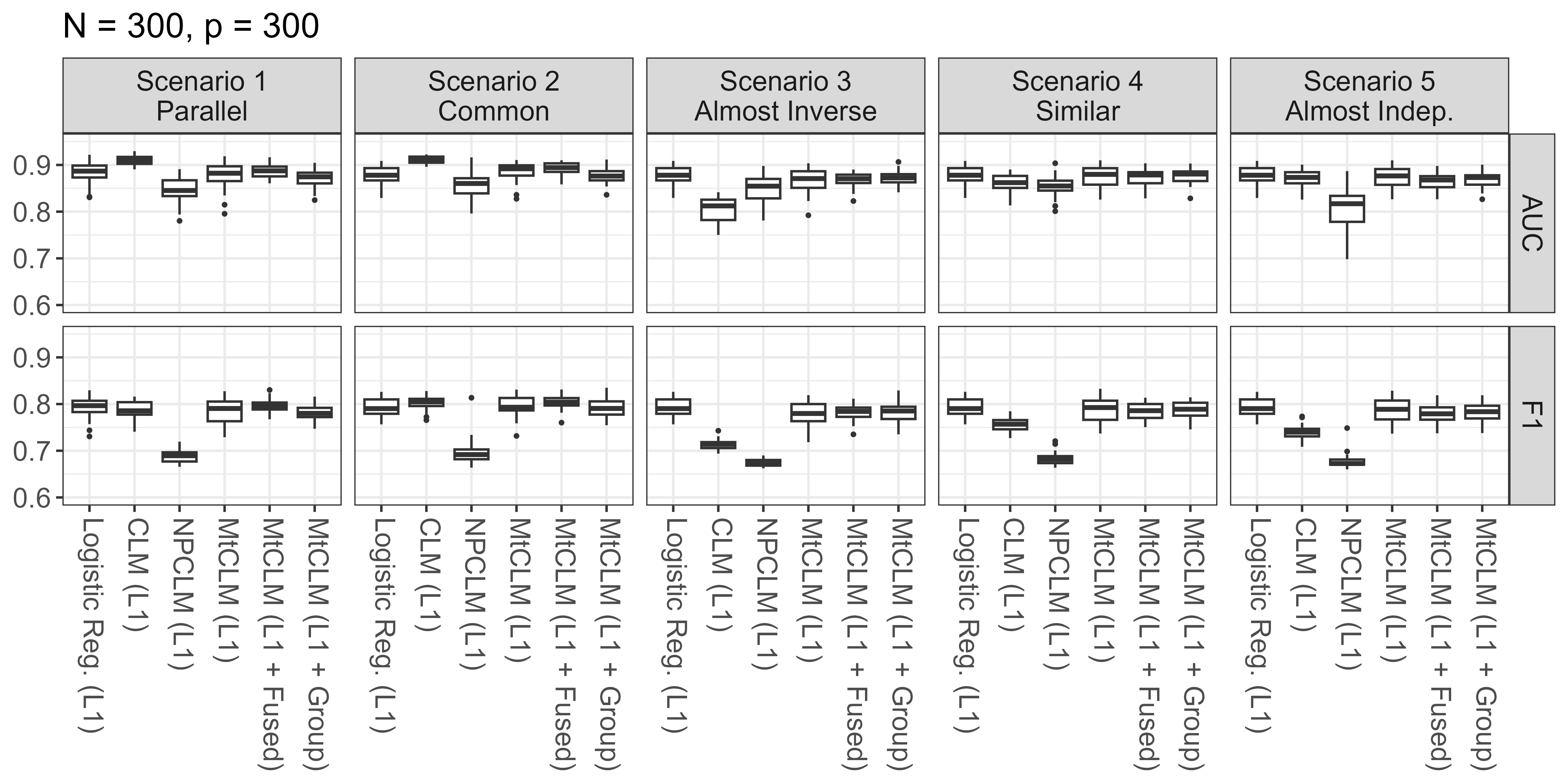
Figure 2 shows the screening performance under the situation with high-dimensional predictors (). The penalized logistic regression, which did not model the severity, showed similar performance across all scenarios and metrics. The penalized CLM exhibited superior performance, particularly in AUC, in Scenario 1, where the parallelism assumption holds, and Scenario 2, where the situation is close to Scenario 1. This result implies that, under appropriate conditions, considering severity can improve screening performance even when tackling a screening task. On the other hand, the NPCLM performed worse than the other methods in all scenarios. This performance degradation can also be attributed to the defect in non-parallel models described in Section 2. Comparing the three MtCLMs, there was no significant difference in screening performance regardless of the penalty used, but the MtCLM (L1) showed slightly larger variability in performance compared to the others. The MtCLM consistently demonstrated performance comparable to or slightly lower than the penalized logistic regression across all scenarios. By making the model more flexible compared to CLM, the performance remained stable even in scenarios where the two tasks had almost no similar structure. Furthermore, in the scenarios with high commonality between tasks (Scenarios 1, 2, and 4), it showed performance comparable to the penalized logistic regression, suggesting that it effectively leveraged the shared structure in appropriate situations despite increased variance due to increased parameters. In the settings with lower dimensional predictors, we obtained similar results; however, it is worth mentioning that the MtCLM slightly outperformed the penalized logistic regression in some scenarios when (See Figure A2 in Appendix Appendix D).

Predictive Performance for the the ordinal responses, namely, the joint task of screening and severity prediction is presented in Figure 3.
As with screening, in Scenarios 1 and 2, where the structure of both tasks is highly similar, the penalized CLM demonstrated high performance. Particularly in terms of Accuracy, the CLM exceeded the others; however, in terms of concordance and MAE, MtCLM (L1 + Fused) was comparable. The penalized NPCLM failed to perform well in all scenarios, and the MtCLM consistently showed high performance across all scenarios, especially in Scenarios 1 and 2 the Fused Lasso penalty worked effectively. The large variance of MtCLM (L1) was also similar to the screening performance results. Besides, MtCLM (L1 + Group) slightly outperformed others in terms of Accuracy in scenarios 3, 4, and 5. When the predictors are of lower dimensions (), MtCLM (particularly L1 + Fused) demonstrated performance equal to or better than CLM in Scenarios 1 and 2. Additionally, in cases where the same variables are related to the response, though in different directions, as in Scenario 3, MtCLM (L1 + Group) performed relatively well.

In variable selection, the results were compared among the variants of MtCLM (Figure 4). Overall, as the dimensionality of the predictors increased, the number of false discoveries also increased. In our settings, all methods were able to select most variables that are truly associated with the response. The FDR varied depending on the choice of penalty term. When using the fused lasso penalty, especially in scenarios 3, 4, and 5, the FDR was very high, and many variables unrelated to the response were selected. When using the L1 penalty alone, the FDR was lower in many scenarios on average, but the variability of the FDR was the highest. When using the group lasso penalty, in scenarios 2 and 3, it showed detection power similar to that of using the L1 penalty alone, and the FDR was relatively lower and more stable than with the fused lasso penalty.

In summary, when there is a hierarchical structure in ordinal responses, if the structures between hierarchies are highly similar, or if the parallelism assumption is believed to hold, CLM is highly effective. Moreover, even when the primary goal is the classification of the first hierarchy, namely screening, modeling the response as an ordinal response including severity may improve screning performance. However, considering the possibility of structural differences between hierarchies, a model that accounts for these differences, such as MtCLM, should be used. As seen across the five scenarios, MtCLM effectively works even in cases where the structures between hierarchies largely differ, even with penalties like the fused lasso that emphasize shared structures. Furthermore, when the structures are well-shared between hierarchies, the fused lasso penalty is particularly effective, performing comparably to CLM. The proposed methods are said to be adaptive to the data and robust to structural differences, as they improve performance by leveraging commonalities between hierarchies when structures are highly shared and fit each task as a different model when commonalities are poor.
6 Real Data Analysis
6.1 Pancreatic Ductal Adenocarcinoma Dataset
In this section, we report the results of applying the proposed methods and some existing methods.
Debernardi et al. (2020) provide an open and cleaned dataset on the concentration of certain proteins in the urine of healthy individuals and patients with pancreatic ductal adenocarcinoma (PDAC) or benign hepatobiliary diseases Debernardi et al. (2020). The dataset was downloaded from Kaggle datasets on July 3rd, 2023 111https://www.kaggle.com/datasets/johnjdavisiv/urinary-biomarkers-for-pancreatic-cancer?resource=download. The Debernardi dataset consists of 590 individuals and includes the concentration of five molecules (creatinine, LYVE1, REG1B, TFF1, REG1A), cancer diagnosis, cancer stage, and certain demographic factors. They reported that a combination of the three molecules, LYVE1, REG1B, and TFF1, showed good predictive performance in detecting PDAC. To combine the tasks of screening and severity prediction, we defined the response variable as summarized in Table 2. For further descriptive information on the dataset, refer to Appendix E.1.
| Levels | Hierarchy | Definition | # of Cases |
|---|---|---|---|
| 0 | 1st | No PDAC, including benign hepatobiliary diseases | 391 |
| 1 | 2nd | PDAC at stages I, IA, and IB | 16 |
| 2 | 2nd | PDAC at stages II, IIA, and IIB | 86 |
| 3 | 2nd | PDAC at stage III | 76 |
| 4 | 2nd | PDAC at stage IV | 21 |
We applied the methods CLM (polr), CLM (L1), MtCLM (L1), MtCLM (L1 + Fused), and MtCLM (L1 + Group) to this composite response, using age and the concentrations of molecules as predictors. Note that REG1A was excluded from the analysis due to the presence of missing values in about half of the cases. For the methods with tuning parameters, we selected them using 5-fold cross-validation.
Table 3 shows the estimated regression coefficients of these methods.
| Model | Regularization | Task | age | creatinine | LYVE1 | REG1B | TFF1 |
|---|---|---|---|---|---|---|---|
| CLM | None | Overall | 0.634 | 2.381 | 0.474 | 0.023 | |
| L1 | Overall | 0.594 | 1.847 | 0.471 | - | ||
| MtCLM | L1 | Screening | 0.711 | 2.001 | 0.594 | 0.113 | |
| Sev. Pred. | - | 0.259 | - | - | - | ||
| L1 + Fused | Screening | 0.677 | 1.761 | 0.582 | 0.066 | ||
| Sev. Pred. | - | 0.241 | - | - | - | ||
| L1 + Group | Screening | 0.680 | 1.666 | 0.592 | 0.089 | ||
| Sev. Pred. | - | 0.249 | - | - | - |
The coefficients of CLM (polr) and CLM (L1) indicated that age, LYVE1, and REG1B were positively associated with the composite response, and that creatinine was negatively associated. On the other hand, the coefficients of the MtCLMs suggested that creatinine was negatively associated with the presence of cancer but positively associated with cancer severity. These inverse relationships can also be observed by the descriptive analysis (see Figure A12). More importantly, while the three molecules were associated with the outcome in the screening model, they showed no association with the cancer severity. Additionally, creatinine has been reported to have a negative association with the presence of pancreatic cancer Boursi et al. (2017); Dong et al. (2018). Our results by MtCLM are consistent with these findings, although it should be noted that these results were about serum creatinine. The association of REG1B with cancer severity disappeared when using the fused and group lasso regularizations. These results suggest that the two tasks, screening and severity prediction, had significantly different structures in Debernardi’s dataset, making MtCLM a more suitable choice.
In interpreting these results, it is important to note that our defined category includes not only healthy individuals but also cases of non-cancer diseases. As shown in Appendix E, there are differences in the distribution of markers between healthy individuals and those with non-cancer diseases.
6.2 METABRIC Cohort Dataset
Breast cancer is a common cancer among women, and its causes and treatments are widely investigated. The Molecular Taxonomy of Breast Cancer International Consortium (METABRIC) provides a database of genetic mutations and transcriptome profiles from over 2,000 breast cancer specimens collected from tumor banks in the UK and Canada. Using the METABRIC dataset, efforts are made to explore distinct subgroups related to clinical characteristics and prognosis of breast cancer (e.g., Curtis et al., 2012; Mukherjee et al., 2018; Rueda et al., 2019).
At the time the METABRIC cohort was conducted, the progression of breast cancer was roughly classified into five stages, from 0 to 4, based on tumor size and lymph node metastasis. Among these, Stages 0 and 1 indicate no lymph node metastasis, while Stages 2 and above include metastasis to lymph nodes and other organs. Lymph node metastasis is used as a key indicator of cancer progression in many types of cancer, as its presence is known to increase the risk of recurrence and metastasis (ACS, 2019).
In this section, as a demonstration of methodology, data analysis was conducted to predicting the presence or absence of lymph node metastasis and the stage, based on genetic mutations and transcriptome profiles. The original dataset is publicly available on cBioPortal (Cerami et al., 2012; Gao et al., 2013; de Bruijn et al., 2023), but for this analysis, a preprocessed version available on Kaggle datasets (Alharbi, 2020) was used. The dataset includes 1,403 cases with non-missing stage information, including 479 cases without lymph node metastasis, 800 cases with lymph node metastasis (Stage 2), 115 cases with lymph node metastasis (Stage 3), and 9 cases with lymph node metastasis (Stage 4). For constructing the prediction model, 701 cases were randomly assigned to the training set, and 702 cases to the validation set. The predictors included 489 types of mRNA levels and 92 gene mutations out of 173, which had at least 10 cases with mutations in the training data. The tuning parameters were selected from based on 5-fold CV.
Table 4 shows the results of evaluating predictions using each model on the validation set. The L1-penalized logistic regression, a benchmark for screening, showed a low F1 Score based on a probability threshold of 0.5 probably due to the high prevalence of cases with lymph node metastasis. CLM and NPCLM underperformed logistic regression in terms of AUC for screening and all measures for overall evaluation including severity prediction. As discussed later, the weak association between the predictors and severity differences in cases with lymph node metastasis in this data led to overfitting. Although NPCLM was flexible, its performance did not significantly improve. MtCLM outperformed both CLM and NPCLM and showed competitive performance with logistic regression for screening. However, for severity prediction, the predicted values were almost independent of the actual values. In fact, for the severity prediction model, no variables were selected except for MtCLM (L1 + Fused), which non-specifically selected many predictors.
| Screening | Overall | ||||
|---|---|---|---|---|---|
| method | AUC | F1 | Accuracy | MAE | Kendall’s tau |
| Logistic Reg. (L1) | 0.627 | 0.054 | - | - | - |
| CLM (L1) | 0.522 | 0.339 | 0.406 | 0.691 | 0.023 |
| NPCLM (L1) | 0.548 | 0.378 | 0.479 | 0.571 | 0.063 |
| MtCLM (L1) | 0.619 | 0.047 | 0.551 | 0.457 | 0.043 |
| MtCLM (L1 + Fused) | 0.635 | 0.083 | 0.556 | 0.453 | 0.080 |
| MtCLM (L1 + Group) | 0.619 | 0.039 | 0.551 | 0.457 | 0.038 |
Figure 5 shows the association of 498 mRNAs with response variables in univariate analysis and the variables selected in the MtCLM (L1 + Group) screening model. Overall, variables strongly associated with the response variable in univariate analysis tended to be selected. For variables selected by other methods, refer to Appendix E.2. For gene mutations, FANCD2 was selected by the L1-penalized logistic regression, MtCLM (L1), and MtCLM (L1 + Group). While a detailed discussion on this gene mutation is beyond the scope of this study, several reports suggest its association with breast cancer (Barroso et al., 2006; Zhang et al., 2010).

7 Discussion
In this study, we have discussed the combined problem of screening and severity prediction, considering that some biomarkers are associated not only with the presence of disease but also with disease severity. To address this problem, we have proposed a multi-task approach with structured sparse regularization, MtCLM, leveraging the shared structure between the two tasks. MtCLM is an ordinal regression model, which is more flexible than CLM, but unlike NPCLM, it is valid across the entire predictor space and interpretable. The performance of MtCLM on prediction and variable selection was verified by simulation, and an example of real data analysis was provided.
This study suggests the usefulness of a multi-task learning approach for tasks that are expected to have shared structures in medicine, such as screening and severity prediction of the same disease. The idea of multi-task learning is not considered to be prevalent in the field of biomedical research. However, many diseases share risk factors and genetic abnormalities (e.g., hyperlipemia is a risk factor for cardiovascular and cerebrovascular diseases (e.g., Kopin and Lowenstein (2017)), and the HER2 gene is amplified in ovarian and gastric cancers in addition to breast cancer (e.g., Gravalos and Jimeno (2008))). Therefore, the idea of multi-task learning that takes advantage of commonalities among tasks may be useful in building prediction models or investigating prognostic factors using limited data.
Acknowledgements
Kazuharu Harada is partially supported by JSPS KAKENHI Grant Number 22K21286. Shuichi Kawano is partially supported by JSPS KAKENHI Grant Numbers JP23K11008, JP23H03352, and JP23H00809. Masataka Taguri is partially supported by JSPS KAKENHI Grant Number 24K14862.
Declaration of Generative AI and AI-assisted technologies in the writing process
During the preparation of this work, the authors used ChatGPT 4/4o (OpenAI Inc.) in order to improve English writing. After using this tool/service, the authors reviewed and edited the content as needed and take full responsibility for the content of the publication.
References
- ACS [2019] American cancer society: Treatment of breast cancer by stage. https://www.cancer.org/cancer/types/breast-cancer/treatment/treatment-of-breast-cancer-by-stage.html, 2019. Accessed: 2024-6-18.
- Agresti [2010] A. Agresti. Analysis of Ordinal Categorical Data. John Wiley & Sons, Apr. 2010.
- Agresti [2015] A. Agresti. Foundations of Linear and Generalized Linear Models. John Wiley & Sons, Jan. 2015.
- Alharbi [2020] R. Alharbi. Kaggle datasets: Breast cancer gene expression profiles (metabric). https://www.kaggle.com/datasets/raghadalharbi/breast-cancer-gene-expression-profiles-metabric, May 2020. Accessed: 2024-6-18.
- Amano et al. [2024] H. Amano, H. Uchida, K. Harada, A. Narita, S. Fumino, Y. Yamada, S. Kumano, M. Abe, T. Ishigaki, M. Sakairi, C. Shirota, T. Tainaka, W. Sumida, K. Yokota, S. Makita, S. Karakawa, Y. Mitani, S. Matsumoto, Y. Tomioka, H. Muramatsu, N. Nishio, T. Osawa, M. Taguri, K. Koh, T. Tajiri, M. Kato, K. Matsumoto, Y. Takahashi, and A. Hinoki. Scoring system for diagnosis and pretreatment risk assessment of neuroblastoma using urinary biomarker combinations. Cancer Sci., Feb. 2024.
- Barroso et al. [2006] E. Barroso, R. L. Milne, L. P. Fernández, P. Zamora, J. I. Arias, J. Benítez, and G. Ribas. FANCD2 associated with sporadic breast cancer risk. Carcinogenesis, 27(9):1930–1937, Sept. 2006.
- Biomarkers Definitions Working Group. [2001] Biomarkers Definitions Working Group. Biomarkers and surrogate endpoints: preferred definitions and conceptual framework. Clin. Pharmacol. Ther., 69(3):89–95, Mar. 2001.
- Boursi et al. [2017] B. Boursi, B. Finkelman, B. J. Giantonio, K. Haynes, A. K. Rustgi, A. D. Rhim, R. Mamtani, and Y.-X. Yang. A clinical prediction model to assess risk for pancreatic cancer among patients with New-Onset diabetes. Gastroenterology, 152(4):840–850.e3, Mar. 2017.
- Boyd et al. [2011] S. Boyd, N. Parikh, E. Chu, B. Peleato, and J. Eckstein. Distributed optimization and statistical learning via the alternating direction method of multipliers. Foundations and Trends® in Machine Learning, 3(1):1–122, 2011.
- Burridge [1981] J. Burridge. A note on maximum likelihood estimation for regression models using grouped data. J. R. Stat. Soc. Series B Stat. Methodol., 43(1):41–45, Sept. 1981.
- Caruana [1997] R. Caruana. Multitask learning. Mach. Learn., 28(1):41–75, July 1997.
- Cerami et al. [2012] E. Cerami, J. Gao, U. Dogrusoz, B. E. Gross, S. O. Sumer, B. A. Aksoy, A. Jacobsen, C. J. Byrne, M. L. Heuer, E. Larsson, Y. Antipin, B. Reva, A. P. Goldberg, C. Sander, and N. Schultz. The cbio cancer genomics portal: an open platform for exploring multidimensional cancer genomics data. Cancer Discov., 2(5):401–404, May 2012.
- Curtis et al. [2012] C. Curtis, S. P. Shah, S.-F. Chin, G. Turashvili, O. M. Rueda, M. J. Dunning, D. Speed, A. G. Lynch, S. Samarajiwa, Y. Yuan, S. Gräf, G. Ha, G. Haffari, A. Bashashati, R. Russell, S. McKinney, METABRIC Group, A. Langerød, A. Green, E. Provenzano, G. Wishart, S. Pinder, P. Watson, F. Markowetz, L. Murphy, I. Ellis, A. Purushotham, A.-L. Børresen-Dale, J. D. Brenton, S. Tavaré, C. Caldas, and S. Aparicio. The genomic and transcriptomic architecture of 2,000 breast tumours reveals novel subgroups. Nature, 486(7403):346–352, Apr. 2012.
- de Bruijn et al. [2023] I. de Bruijn, R. Kundra, B. Mastrogiacomo, T. N. Tran, L. Sikina, T. Mazor, X. Li, A. Ochoa, G. Zhao, B. Lai, A. Abeshouse, D. Baiceanu, E. Ciftci, U. Dogrusoz, A. Dufilie, Z. Erkoc, E. Garcia Lara, Z. Fu, B. Gross, C. Haynes, A. Heath, D. Higgins, P. Jagannathan, K. Kalletla, P. Kumari, J. Lindsay, A. Lisman, B. Leenknegt, P. Lukasse, D. Madela, R. Madupuri, P. van Nierop, O. Plantalech, J. Quach, A. C. Resnick, S. Y. A. Rodenburg, B. A. Satravada, F. Schaeffer, R. Sheridan, J. Singh, R. Sirohi, S. O. Sumer, S. van Hagen, A. Wang, M. Wilson, H. Zhang, K. Zhu, N. Rusk, S. Brown, J. A. Lavery, K. S. Panageas, J. E. Rudolph, M. L. LeNoue-Newton, J. L. Warner, X. Guo, H. Hunter-Zinck, T. V. Yu, S. Pilai, C. Nichols, S. M. Gardos, J. Philip, AACR Project GENIE BPC Core Team, AACR Project GENIE Consortium, K. L. Kehl, G. J. Riely, D. Schrag, J. Lee, M. V. Fiandalo, S. M. Sweeney, T. J. Pugh, C. Sander, E. Cerami, J. Gao, and N. Schultz. Analysis and visualization of longitudinal genomic and clinical data from the AACR project GENIE biopharma collaborative in cBioPortal. Cancer Res., 83(23):3861–3867, Dec. 2023.
- Debernardi et al. [2020] S. Debernardi, H. O’Brien, A. S. Algahmdi, N. Malats, G. D. Stewart, M. Plješa-Ercegovac, E. Costello, W. Greenhalf, A. Saad, R. Roberts, A. Ney, S. P. Pereira, H. M. Kocher, S. Duffy, O. Blyuss, and T. Crnogorac-Jurcevic. A combination of urinary biomarker panel and PancRISK score for earlier detection of pancreatic cancer: A case-control study. PLoS Med., 17(12):e1003489, Dec. 2020.
- Dong et al. [2018] X. Dong, Y. B. Lou, Y. C. Mu, M. X. Kang, and Y. L. Wu. Predictive factors for differentiating pancreatic cancer-associated diabetes mellitus from common type 2 diabetes mellitus for the early detection of pancreatic cancer. Digestion, 98(4):209–216, July 2018.
- for the Study of the Liver [2018] E. A. for the Study of the Liver. Easl clinical practice guidelines: Management of hepatocellular carcinoma. J. Hepatol., 69(1):182–236, July 2018.
- Gao et al. [2013] J. Gao, B. A. Aksoy, U. Dogrusoz, G. Dresdner, B. Gross, S. O. Sumer, Y. Sun, A. Jacobsen, R. Sinha, E. Larsson, E. Cerami, C. Sander, and N. Schultz. Integrative analysis of complex cancer genomics and clinical profiles using the cBioPortal. Sci. Signal., 6(269):l1, Apr. 2013.
- Gravalos and Jimeno [2008] C. Gravalos and A. Jimeno. HER2 in gastric cancer: a new prognostic factor and a novel therapeutic target. Ann. Oncol., 19(9):1523–1529, Sept. 2008.
- Hastie et al. [2015] T. Hastie, R. Tibshirani, and M. Wainwright. Statistical Learning with Sparsity. Chapman and Hall/CRC, 2015.
- Irwin et al. [2021] M. S. Irwin, A. Naranjo, F. F. Zhang, S. L. Cohn, W. B. London, J. M. Gastier-Foster, N. C. Ramirez, R. Pfau, S. Reshmi, E. Wagner, J. Nuchtern, S. Asgharzadeh, H. Shimada, J. M. Maris, R. Bagatell, J. R. Park, and M. D. Hogarty. Revised neuroblastoma risk classification system: A report from the children’s oncology group. J. Clin. Oncol., 39(29):3229, Oct. 2021.
- Jani et al. [2017] P. D. Jani, L. Forbes, A. Choudhury, J. S. Preisser, A. J. Viera, and S. Garg. Evaluation of diabetic retinal screening and factors for ophthalmology referral in a telemedicine network. JAMA Ophthalmol., 135(7):706–714, July 2017.
- Kopin and Lowenstein [2017] L. Kopin and C. Lowenstein. Dyslipidemia. Ann. Intern. Med., 167(11):ITC81–ITC96, Dec. 2017.
- McCullagh [1980] P. McCullagh. Regression models for ordinal data. J. R. Stat. Soc. Series B Stat. Methodol., 42(2):109–142, 1980.
- Muchie [2016] K. F. Muchie. Determinants of severity levels of anemia among children aged 6–59 months in ethiopia: further analysis of the 2011 ethiopian demographic and health survey. BMC Nutrition, 2(1):1–8, Aug. 2016.
- Mukherjee et al. [2018] A. Mukherjee, R. Russell, S.-F. Chin, B. Liu, O. M. Rueda, H. R. Ali, G. Turashvili, B. Mahler-Araujo, I. O. Ellis, S. Aparicio, C. Caldas, and E. Provenzano. Associations between genomic stratification of breast cancer and centrally reviewed tumour pathology in the METABRIC cohort. NPJ Breast Cancer, 4:5, Mar. 2018.
- Okuno and Harada [2024] A. Okuno and K. Harada. An interpretable neural network-based non-proportional odds model for ordinal regression. J. Comput. Graph. Stat., pages 1–23, Feb. 2024.
- Omata et al. [2017] M. Omata, A.-L. Cheng, N. Kokudo, M. Kudo, J. M. Lee, J. Jia, R. Tateishi, K.-H. Han, Y. K. Chawla, S. Shiina, W. Jafri, D. A. Payawal, T. Ohki, S. Ogasawara, P.-J. Chen, C. R. A. Lesmana, L. A. Lesmana, R. A. Gani, S. Obi, A. K. Dokmeci, and S. K. Sarin. Asia-Pacific clinical practice guidelines on the management of hepatocellular carcinoma: a 2017 update. Hepatol. Int., 11(4):317–370, July 2017.
- Peterson and Harrell [1990] B. Peterson and F. E. Harrell. Partial proportional odds models for ordinal response variables. J. R. Stat. Soc. Series C Appl. Stat., 39(2):205–217, 1990.
- Pratt [1981] J. W. Pratt. Concavity of the log likelihood. J. Am. Stat. Assoc., 76(373):103–106, Mar. 1981.
- Rueda et al. [2019] O. M. Rueda, S.-J. Sammut, J. A. Seoane, S.-F. Chin, J. L. Caswell-Jin, M. Callari, R. Batra, B. Pereira, A. Bruna, H. R. Ali, E. Provenzano, B. Liu, M. Parisien, C. Gillett, S. McKinney, A. R. Green, L. Murphy, A. Purushotham, I. O. Ellis, P. D. Pharoah, C. Rueda, S. Aparicio, C. Caldas, and C. Curtis. Dynamics of breast-cancer relapse reveal late-recurring ER-positive genomic subgroups. Nature, 567(7748):399–404, Mar. 2019.
- Simon et al. [2013] N. Simon, J. Friedman, T. Hastie, and R. Tibshirani. A Sparse-Group lasso. J. Comput. Graph. Stat., 22(2):231–245, Apr. 2013.
- Tibshirani [1996] R. Tibshirani. Regression shrinkage and selection via the lasso. J. R. Stat. Soc. Series B Stat. Methodol., 58(1):267–288, Jan. 1996.
- Tibshirani et al. [2005] R. Tibshirani, M. Saunders, S. Rosset, J. Zhu, and K. Knight. Sparsity and smoothness via the fused lasso. J. R. Stat. Soc. Series B Stat. Methodol., 67(1):91–108, Feb. 2005.
- Tibshirani and Taylor [2011] R. J. Tibshirani and J. Taylor. The solution path of the generalized lasso. Ann. Stat., 39(3):1335–1371, June 2011.
- Tugnait [2021] J. K. Tugnait. Sparse-Group lasso for graph learning from Multi-Attribute data. IEEE Trans. Signal Process., 69:1771–1786, 2021.
- Tutz and Gertheiss [2016] G. Tutz and J. Gertheiss. Regularized regression for categorical data. Stat. Modelling, 16(3):161–200, June 2016.
- Wang et al. [2020] Z. Wang, Z. He, M. Shah, T. Zhang, D. Fan, and W. Zhang. Network-based multi-task learning models for biomarker selection and cancer outcome prediction. Bioinformatics, 36(6):1814–1822, Mar. 2020.
- Wurm et al. [2021] M. J. Wurm, P. J. Rathouz, and B. M. Hanlon. Regularized ordinal regression and the ordinalnet R package. J. Stat. Softw., 99(6), Sept. 2021.
- Xiao et al. [2023] Y. Xiao, L. Zhang, B. Liu, R. Cai, and Z. Hao. Multi-task ordinal regression with labeled and unlabeled data. Inf. Sci., 649:119669, Nov. 2023.
- Yuan and Lin [2006] M. Yuan and Y. Lin. Model selection and estimation in regression with grouped variables. J. R. Stat. Soc. Series B Stat. Methodol., 68(1):49–67, 2006.
- Zhang et al. [2010] B. Zhang, R. Chen, J. Lu, Q. Shi, X. Zhang, and J. Chen. Expression of FANCD2 in sporadic breast cancer and clinicopathological analysis. J. Huazhong Univ. Sci. Technolog. Med. Sci., 30(3):322–325, June 2010.
- Zhang and Ip [2012] Q. Zhang and E. H. Ip. Generalized linear model for partially ordered data. Stat. Med., 31(1):56–68, Jan. 2012.
- Zhang and Yang [2017] Y. Zhang and Q. Yang. An overview of multi-task learning. Natl Sci Rev, 5(1):30–43, Sept. 2017.
Appendix Appendix A Further Illustrations for the Learning with Structural Sparse Regularization

Appendix Appendix B Details of ADMM Algorithm
Appendix B.1 ADMM for Group lasso-type Estimation
In this subsection, we derive the ADMM algorithm for the problem (12). The optimization problem (12) is equivalent to the following problem, which introduces a redundant parameter .
| (A3) |
where are row vectors of . The augmented Lagrangian of this problem is defined as
| (A4) |
where is a Lagrange multilier and is a tuning parameter for optimization. In ADMM, the parameters are updated in sequence to minimize (A4). The Lagrange multipliers are updated by the gradient descent. Given the parameters of the previous step, the updating formulae are given below:
| (A5) | ||||
| (A6) | ||||
| (A7) |
The small problem (A5) does not have an explicit solution, so it has to be solved by an iterative algorithm. Since the target function of (A5) is convex, it can be solved using an off-the-shelf solver. The problems (A6) can be solved in the following 2-step procedure Simon et al. [2013], Tugnait [2021]:
and
where is the soft-thresholding operator for a group lasso-type penalty, and is the th row vector of . Repeat steps (A5) through (A7) until an appropriate convergence criterion is met to obtain the final estimate.
Appendix B.2 Gradient of the Augmented Langrangian
We derive the gradient of the augmented Lagrangian for the fused lasso-type problem. Note that the derivative of is , which is also the density function of the logistic distribution. Each gradient is given as follows:
Since and , we have .
For the group lasso-type augmented Lagrangian, some modifications are needed. Let and be the column vectors of , and then the gradients are
Appendix Appendix C Details on the Numerical Experiments
Appendix C.1 Simulation Models
The datasets for the numerical experiments are generated from the CLM and MtCLM models. Specifically, the ordinal response is generated by discretizing continuous variables and into four categories (for the scenario of CLM, we only generate ). and are generated by adding error terms that follow a standard logistic distribution to the linear combinations of the predictors. The discretization thresholds are set so that the four categories comprise 50%, 16.7%, 16.7%, and 16.7% of the data, respectively. All predictors are generated from a -dimensional multivariate normal distribution, where they are mutually independent. The dimension is in . In the case of CLM, 10 out of the regression coefficients were set to non-zero, while in the case of MtCLM, 10 out of the total regression coefficients for each task are set to non-zero. The absolute values of the non-zero regression coefficients were drawn from a uniform distribution over . The selection and sign of the non-zero regression coefficients depend on the following scenarios.
Scenario 1: Parallel
The simulation model is a parallel CLM, where among the 10 non-zero coefficients, the first 5 are positively associated with , and the remaining 5 are negatively associated with .
Scenario 2: Identical
The simulation model is a MtCLM. All relevant predictors have regression coefficients with the same signs in screening and severity prediction. Among the non-zero coefficients for each task, the first 5 are positively associated with , and the remaining 5 are negatively associated with .
Scenario 3: Almost Inverse
The simulation model is an MtCLM. The relevant predictors are common in both screening and severity prediction, but the signs of the regression coefficients are almost inverse for each task. Specifically, among the 10 non-zero coefficients for the screening model, the first 5 coefficients are positive, and the remaining 5 are negative. In contrast, the signs are inverse in the severity model, except for the 1st and 6th coefficients.
Scenario 4: Similar
The simulation model is an MtCLM. Many of the relevant predictors are common between the screening and severity models, but some are different. Specifically, among the 10 non-zero coefficients for the screening model, the first 5 coefficients are positive, and the remaining 5 are negative. For the severity model, the same predictors are associated with the response in the same direction, except for the 4th and 9th. Instead of the 4th and 9th predictors, the 11th and 12th predictors are associated with the response.
Scenario 5: Almost Independent
The simulation model is an MtCLM. Only two predictors are shared between both tasks. Specifically, among the 10 non-zero coefficients for the screening model, the first 5 coefficients are positive, and the remaining 5 are negative. For the severity model, only the 1st and 6th predictors are associated with the response in the same direction, whereas the 11th to 14th predictors are positively associated with severity, and the 15th to 18th predictors are negatively associated with severity.
Appendix C.2 Evaluation Measures
We use the following evaluation measures to evaluate the predictive performance. The ROC-AUC and the F1 score are used to evaluate performance in screening, and the accuracy, MAR, and Kendall’s tau are used to evaluate performance in the combined task of screening and severity prediction.
-
•
ROC-AUC: the area under the curve for the receiver operating characteristic. We simply refer to it as AUC. This takes values in and it measures the overall performance for the binary classification of a continuous indicator, taking into account sensitivity and specificity on various cutoff values.
-
•
F1 Score: the harmonic mean of the positive predictive value (PPV, or Precision) and the sensitivity (or Recall), which measures the overall performance for the binary classification of a specific rule.
-
•
Accuracy: the proportion of the accurate prediction across all levels of the ordinal response.
-
•
MAE: the mean absolute error for the ordinal response.
-
•
Kendall’s tau: a statistic that measures the ordinal association between two quantities and is one measure of concordance. A value of indicates complete disagreement, 0 indicates no association, and 1 indicates complete agreement.
To evaluate the variable selection performance, we use the following measures.
-
•
F1 Score
-
•
False Discovery Rate (FDR): False Positive / Predicted Positive.
-
•
Sensitivity: True Positive / Positive.
-
•
Specificity: True Negative / Negative.
Appendix Appendix D Additional Results for Numerical Experiments
In addition to the setting with presented in the main text, comparisons were also conducted for .


Appendix Appendix E Further Information of Real Data Analysis
Appendix E.1 Pancreatic Ductal Adenocarcinoma Dataset


Appendix E.2 METABRIC Cohort Dataset


