Simultaneous Mode, Input and State Set-Valued Observers with Applications to Resilient Estimation against Sparse Attacks

Mohammad Khajenejad Sze Zheng Yong
^a Mohammad Khajenejad and Sze Zheng Yong are with the School for Engineering of Matter, Transport and Energy, Arizona State University, Tempe, AZ, USA (e-mail: [email protected], [email protected]).

Abstract

A simultaneous mode, input and state set-valued observer is proposed for hidden mode switched linear systems with bounded-norm noise and unknown input signals. The observer consists of two constituents: (i) a bank of mode-matched observers and (ii) a mode estimator. Each mode-matched observer recursively outputs the mode-matched sets of compatible states and unknown inputs, while the mode estimator eliminates incompatible modes, using a residual-based criterion. Then, the estimated sets of states and unknown inputs are the union of the mode-matched estimates over all compatible modes. Moreover, sufficient conditions to guarantee the elimination of all false modes are provided and the effectiveness of our approach is exhibited using an illustrative example.

I Introduction

Potential vulnerability of Cyber-Physical Systems (CPS) to adversarial attacks and henceforth their security, are emerging as an important and critical issue. Given that attackers are often strategic, there are many potential avenues through which they can cause harm, steal information/power, etc. Recent incidents of attacks on CPS, e.g., the Maroochy water system and Ukrainian power grid, [1, 2], highlight a need for new resilient estimation and control designs.

In particular, an adversary’s ability to inject counterfeit data into sensor and actuator signals (false data injection) or to compromise an unknown subset of vulnerable sensors and actuators (e.g., [3, 4, 5, 6, 7, 8, 9]) in order to mislead the system operator has been a subject of considerable interest in recent years. This problem can be considered in a more general framework of hidden mode switched linear systems with unknown inputs and also has applications in urban transportation systems [6], aircraft tracking and fault detection [10], etc.

Literature review. The filtering problem of hidden mode systems without unknown inputs have been extensively studied (see, e.g., [11, 12] and references therein). More recently, an extension to consider unknown inputs has been proposed in [6] for stochastic systems. However, these methods mainly focus on obtaining point estimates, i.e., the most likely or best single estimates, and do not directly apply to bounded-error models, i.e., uncertain dynamic systems with set-valued uncertainties (e.g., bounded-norm noise), where the sets of all modes, states and unknown inputs that are compatible with sensor observations are desired.

On the other hand, set-membership or set-valued state observers (e.g., [13, 14, 15]) are capable of estimating the set of compatible states and are preferable to stochastic estimation when hard accuracy bounds are important, e.g., to guarantee safety. Moreover, a recent extension to also compute the set of unknown input signals in addition to the states has been introduced in [16]. However, these approaches do not apply to hidden mode systems that we consider in this paper.

In the context of resilient estimation against sparse false data injection attacks, numerous approaches were proposed (e.g., [3, 4, 5, 6, 7, 8, 9]), but they all only obtain point estimates, as opposed to set-valued estimate s. Moreover, only sensor attacks have been considered, although actuator attacks are also a source of concern in CPS security. On the other hand, our prior work in [16, 17] design a fixed-order set-valued observer that simultaneously outputs sets of compatible state and input estimates despite data injection attacks for linear time-invariant and linear parameter-varying systems, without considering the hidden modes, i.e., with the assumption that the subset of attacked sensors and actuators is known.

To consider hidden modes, a common approach is to construct residual signals, especially for fault detection [18], where a threshold based on the residual signal is used to distinguish between consistent and inconsistent modes. Using this idea, [19] presents a robust control inspired resilient state estimator for models with bounded-norm noise that consists of local estimators, residual detectors and a global fusion detector. However, in their setting, only sensors are attacked, while the existence of the observers are assumed with no observer design approach nor performance guarantees.

Contributions. The goal of this paper is to simultaneously consider state and unknown input estimation as well as mode detection for hidden mode switched linear systems with bounded-norm noise and unknown inputs. To address this, we propose a multiple-model approach that leverages the optimally designed set-valued state and input $\mathcal{H}_{\infty}$ observers in our previous work [16] to obtain a bank of mode-matched set-valued observers in combination with a novel mode observer based on elimination. Our mode elimination approach uses the upper bound of the norm of to-be-designed residual signals to remove inconsistent modes from the bank of observers. In particular, we provide a tractable method to calculate an upper bound signal for the residual’s norm and prove that the upper bound signal is a convergent sequence. Moreover, we provide sufficient conditions to guarantee that all false modes will be eventually eliminated.

Notation. $\mathbb{R}^{n}$ denotes the $n$ -dimensional Euclidean space and $\mathbb{N}$ nonnegative integers. For a vector $v\in\mathbb{R}^{n}$ and a matrix $M\in\mathbb{R}^{p\times q}$ , $\|v\|_{2}\triangleq\sqrt{v^{\top}v}$ , $\|v\|_{\infty}\triangleq\max\limits_{1\leq i\leq n}v_{i}$ and $\|M\|_{2}$ and $\sigma_{\min}(M)$ denote their induced $2$ -norm and non-trivial least singular value, respectively.

II Problem Statement

Consider a hidden mode switched linear system with bounded-norm noise and unknown inputs (i.e., a hybrid system with linear and noisy system dynamics in each mode, and the mode and some inputs are not known/measured):

\displaystyle\begin{array}[]{ll}x_{k+1}&=Ax_{k}+Bu^{q}_{k}+G^{q}d^{q}_{k}+w_{k},\\ y_{k}&=Cx_{k}+Du^{q}_{k}+H^{q}d^{q}_{k}+v_{k},\end{array}

(3)

where $x_{k}\in\mathbb{R}^{n}$ is the continuous system state and $q\in\mathbb{Q}=\{1,2,\dots,Q\}$ is the hidden discrete state or mode. For each (fixed) mode $q$ , $u^{q}_{k}\in U^{q}_{k}\subset\mathbb{R}^{m}$ is the known input, $d^{q}_{k}\in\mathbb{R}^{p}$ the unknown but sparse input or attack signal, i.e., every vector $d^{q}_{k}$ has precisely $\rho\in\mathbb{N}$ nonzero elements where $\rho$ is a known parameter, $y_{k}\in\mathbb{R}^{l}$ is the output, whereas $w_{k}\in\mathbb{R}^{n}$ and $v_{k}\in\mathbb{R}^{l}$ are process and measurement 2-norm bounded disturbances with known parameters $\eta_{w}$ and $\eta_{v}$ as their 2-norm bounds respectively. The matrices $A\in\mathbb{R}^{n\times n}$ , $B\in\mathbb{R}^{n\times m}$ , $G^{q}\in\mathbb{R}^{n\times p}$ , $C\in\mathbb{R}^{l\times n}$ , $D\in\mathbb{R}^{l\times m}$ and $H^{q}\in\mathbb{R}^{l\times p}$ are known and no prior ‘useful’ knowledge or assumption of the dynamics of $d^{q}_{k}$ , except sparsity is assumed.

More precisely, $G^{q}$ and $H^{q}$ represent the different hypothesis for each mode $q\in\mathbb{Q}$ , about the sparsity pattern of the unknown inputs, which in the context of sparse attacks corresponds to which actuators and sensors are attacked or not attacked. In other words, we assume that $G^{q}=G\mathbb{I}^{q}_{G}$ and $H^{q}=H\mathbb{I}^{q}_{H}$ for some input matrices $G\in\mathbb{R}^{n\times t_{a}}$ and $H\in\mathbb{R}^{l\times t_{s}}$ , where $t_{a}$ and $t_{s}$ are the number of vulnerable actuator and sensor signals respectively. Note that $\rho^{q}_{a}\leq t_{a}\leq m$ and $\rho^{q}_{s}\leq t_{s}\leq l$ , where $\rho^{q}_{a}$ ( $\rho^{q}_{s}$ ) is the number of attacked actuator (sensor) signals and clearly cannot exceed the number of vulnerable actuator (sensor) signals, which in turn cannot exceed the total number of actuators (sensors). Furthermore, we assume that the total number of unknown inputs/attacks in each mode is known and equals $\rho=\rho_{a}+\rho_{s}$ (sparsity assumption). Moreover, the index matrix $\mathbb{I}^{q}_{G}\in\mathbb{R}^{t_{a}\times\rho}$ ( $\mathbb{I}^{q}_{H}\in\mathbb{R}^{t_{s}\times\rho}$ ) represents the sub-vector of $d_{k}\in\mathbb{R}^{\rho}$ that indicates signal magnitude attacks on the actuators (sensors).

Note that the approach in our paper can be easily extended to handle mode-dependent $A$ , $B$ , $C$ , $D$ , $w_{k}$ , $v_{k}$ , $\eta_{w}$ and $\eta_{v}$ but is omitted to simplify the notation. Moreover, throughout the paper, we assume, without loss of generality, that for each possible mode $q$ , the system $(A,G^{q},C,H^{q})$ is strongly detectable [16, Definition 1], since this is a necessary and sufficient condition for obtaining meaningful set-valued state and input estimates when the mode is known.

Using the modeling framework above, the simultaneous state, unknown input and hidden mode estimation problem is threefold and can be stated as follows:

Problem 1.

Given a switched linear hidden mode discrete-time bounded-error system with unknown inputs (3),

1.

Design a bank of mode-matched observers that for each mode optimally finds the set estimates of compatible states and unknown inputs in the minimum $\mathcal{H}_{\infty}$ -norm sense, i.e., with minimum average power amplification, conditional on the mode being true.
2.

Develop a mode observer via elimination and the corresponding criterion to eliminate false modes.
3.

Find sufficient conditions for eliminating all false modes.

III Proposed Observer Design

In this section, we propose a multiple-model approach for simultaneous mode, state and unknown input estimation for (3), where the goal of the observer is to find compatible set estimates $\hat{D}_{k}$ , $\hat{X}_{k}$ and $\hat{\mathbb{Q}}_{k}$ for unknown inputs, states and modes at time step $k$ , respectively.

III-A Overview of Multiple-Model Approach

The multiple-model design approach consists of three components: (i) designing a bank of mode-matched set-valued observers, (ii) designing a mode observer for eliminating incompatible modes using residual detectors, and (iii) a global fusion observer that outputs the desired set-valued mode, input and state estimates.

III-A1 Mode-Matched Set-Valued Observer

First, we design a bank of mode-matched observers, which consists of $Q$ simultaneous state and input $\mathcal{H}_{\infty}$ set-valued observers based on the optimal fixed-order observer design in [16], which we briefly summarize here. For each mode-matched observer corresponding to mode $q$ , following the approach in [16, Section 3.1], we consider set-valued fixed-order estimates of the form:

	$\displaystyle\hat{D}^{q}_{k-1}$	$\displaystyle=\{d_{k-1}\in\mathbb{R}^{p}:\\|d_{k-1}-\hat{d}^{q}_{k-1}\\|\leq\delta^{d,q}_{k-1}\},$		(4)
	$\displaystyle\hat{X}^{q}_{k}$	$\displaystyle=\{x_{k}\in\mathbb{R}^{n}:\\|x_{k}-\hat{x}^{q}_{k\|k}\\|\leq\delta^{x,q}_{k}\},$		(5)

where their centroids are obtained with the following three-step recursive observer that is optimal in $\mathcal{H}_{\infty}$ -norm sense:

Unknown Input Estimation:

\displaystyle\begin{array}[]{rl}\hat{d}^{q}_{1,k}&=M^{q}_{1}(z^{q}_{1,k}-C^{q}_{1}\hat{x}^{q}_{k|k}-D^{q}_{1}u^{q}_{k})\\ \hat{d}^{q}_{2,k-1}&=M^{q}_{2}(z^{q}_{2,k}-C^{q}_{2}\hat{x}^{q}_{k|k-1}-D^{q}_{2}u^{q}_{k})\\ \hat{d}^{q}_{k-1}&=V^{q}_{1}\hat{d}^{q}_{1,k-1}+V^{q}_{2}\hat{d}^{q}_{2,k-1}\end{array}

(9)

Time Update:

\displaystyle\begin{array}[]{rl}\hat{x}^{q}_{k|k-1}&=A\hat{x}^{q}_{k-1|k-1}+Bu^{q}_{k-1}+G^{q}_{1}\hat{d}^{q}_{1,k-1}\\ \hat{x}^{\star,q}_{k|k}&=\hat{x}^{q}_{k|k-1}+G^{q}_{2}\hat{d}^{q}_{2,k-1}\end{array}

(12)

Measurement Update:

\displaystyle\hat{x}^{q}_{k|k}

\displaystyle=\hat{x}^{\star,q}_{k|k}+\tilde{L}^{q}(z^{q}_{2,k}-C^{q}_{2}\hat{x}^{\star,q}_{k|k}-D^{q}_{2}u^{q}_{k})\quad

(13)

where $\tilde{L}^{q}\in\mathbb{R}^{n\times(l-p_{H^{q}})}$ , $M^{q}_{1}\in\mathbb{R}^{p_{H^{q}}\times p_{H^{q}}}$ and $M^{q}_{2}\in\mathbb{R}^{(p-p_{H^{q}})\times(l-p_{H^{q}})}$ are observer gain matrices that are chosen in the following theorem from [16] to minimize the “volume” of the set of compatible states and unknown inputs, quantified by the radii $\delta^{d,q}_{k-1}$ and $\delta_{k}^{x,q}$ .

Theorem 1.

[16, Lemma 2 & Theorem 4] Suppose the system $(A,G^{q},C,H^{q})$ is strongly detectable, $M^{q}_{1}\Sigma^{q}=I$ and $M^{q}_{2}C^{q}_{2}G^{q}_{2}=I$ . Then, for each mode $q$ , there exists a stable and optimal (in $\mathcal{H}_{\infty}$ -norm sense) observer with gain $\tilde{L}^{q}$ , where the input and state estimation errors, $\tilde{d}^{q}_{k-1}\triangleq d^{q}_{k-1}-\hat{d}^{q}_{k-1}$ and $\tilde{x}^{q}_{k|k}\triangleq x_{k}-\hat{x}^{q}_{k|k}$ , are bounded for all $k$ (i.e., the set-valued estimates are bounded with radii $\delta^{d,q}_{k-1},\delta_{k}^{x,q}<\infty$ ), and the observer gains and the set estimates are given in [16, Theorem 2 & Algorithm 1].

III-A2 Mode Estimation Observer

To estimate the set of compatible modes, we consider an elimination approach that compares residual signals against some thresholds. Specifically, we will eliminate a specific mode $q$ , if $\|r^{q}_{k}\|_{2}>\hat{\delta}^{q}_{r,k}$ , where the residual signal $r^{q}_{k}$ is defined as follows and the thresholds $\hat{\delta}^{q}_{r,k}$ will be derived in Section III-B.

Definition 1 (Residuals).

For each mode $q$ at time step $k$ , the residual signal is defined as:

\displaystyle r^{q}_{k}\triangleq z^{q}_{2,k}-C^{q}_{2}\hat{x}^{\star,q}_{k|k}-D^{q}_{2}u^{q}_{k}.

III-A3 Global Fusion Observer

Then, combining the outputs of both components above, our proposed global fusion observer will provide mode, unknown input and state set-valued estimates at each time step $k$ as:

\displaystyle\begin{array}[]{c}\hat{\mathbb{Q}}_{k}=\{q\in\mathbb{Q}\ \vline\ \|r^{q}_{k}\|_{2}\leq\hat{\delta}^{q}_{r,k}\},\\ \hat{D}_{k-1}=\cup_{q\in\hat{\mathbb{Q}}_{k}}D^{q}_{k-1},\ \hat{X}_{k}=\cup_{q\in\hat{\mathbb{Q}}_{k}}X^{q}_{k}.\end{array}

The multiple-model approach is summarized in Algorithm 1.

Algorithm 1 Simultaneous Mode, State and Input Estimation

\hat{\mathbb{Q}}_{0}=\mathbb{Q}

;

2:for

k=1

N

3: for

q\in\hat{\mathbb{Q}}_{k-1}

\triangleright

Mode-Matched State and Input Set-Valued Estimates

5: Compute

T^{q}_{2},M^{q}_{1},M^{q}_{2},\tilde{L}^{q},\hat{x}^{\star,q}_{k|k},\hat{X}^{q}_{k},\hat{D}^{q}_{k-1}

via Theorem 1;

z^{q}_{2,k}=T^{q}_{2}y_{k}

;

\triangleright

Mode Observer via Elimination

\hat{\mathbb{Q}}_{k}=\hat{\mathbb{Q}}_{k-1}

;

9: Compute

r^{q}_{k}

via Definition 1 and

\hat{\delta}^{q}_{r,k}

via Theorem 3;

10: if

\|r^{q}_{k}\|_{2}>\hat{\delta}^{q}_{r,k}

then

\hat{\mathbb{Q}}_{k}=\hat{\mathbb{Q}}_{k}\backslash\{q\}

;

11: end if

12: end for

13:

\triangleright

State and Input Estimates

14:

\hat{X}_{k}=\cup_{q\in\hat{\mathbb{Q}}_{k}}\hat{X}^{q}_{k}

;

\hat{D}_{k}=\cup_{q\in\hat{\mathbb{Q}}_{k}}\hat{D}^{q}_{k}

;

15:end for

III-B Mode Elimination Approach

The idea is simple. If the residual signal of a particular mode exceeds its upper bound conditioned on this mode being true, we can conclusively rule it out as incompatible. To do so, for each mode $q$ , we first compute an upper bound ( $\hat{\delta}^{q}_{r,k}$ ) for the 2-norm of its corresponding residual at time $k$ , conditioned on $q$ being the true mode. Then, comparing the 2-norm of residual signal in Definition 1 with $\hat{\delta}^{q}_{r,k}$ , we can eliminate mode $q$ if the residual’s 2-norm is strictly greater than the upper bound. This can be formalized using the following proposition and theorem.

Proposition 1.

Consider mode $q$ at time step $k$ , its residual signal $r^{q}_{k}$ (as defined in Definition 1) and the unknown true mode $q^{*}$ . Then,

	$\displaystyle r^{q}_{k}=r^{q\|}_{k}+\Delta r^{q\|q}_{k},\textstyle{where}$
	$\displaystyle r^{q\|}_{k}\triangleq z^{q}_{2,k}-C^{q}_{2}\hat{x}^{\star,q}_{k\|k}-D^{q}_{2}u^{q}_{k}=T^{q*}_{2}y_{k}-C^{q}_{2}\hat{x}^{\star,q}_{k\|k}-D^{q}_{2}u^{q}_{k},$
	$\displaystyle\Delta r^{q\|q}_{k}\triangleq(T^{q}_{2}-T^{q}_{2})y_{k},$

where $r^{q|*}_{k}$ is the true mode’s residual signal (i.e., $q=q^{*}$ ), and $\Delta r^{q|q^{*}}_{k}$ is the residual error.

Proof.

This follows directly from plugging the above expressions into the right hand side term of Definition 1. ∎

Theorem 2.

Consider mode $q$ and its residual signal $r^{q}_{k}$ at time step $k$ . Assume that $\delta^{q,*}_{r,k}$ is any signal that satisfies $\|r^{q|*}_{k}\|_{2}\leq\delta^{q,*}_{r,k}$ , where $r^{q|*}_{k}$ is defined in Proposition 1. Then, mode $q$ is not the true mode, i.e., can be eliminated at time $k$ , if $\|r^{q}_{k}\|_{2}>\delta^{q,*}_{r,k}.$

Proof.

To use contradiction, suppose $q$ is the true mode. By uniqueness of the true mode $q=q^{*}$ , so $T^{q}_{2}=T^{q*}_{2}$ and by Proposition 1, $\Delta r^{q|q*}_{k}=0$ and hence $\|r^{q}_{k}\|_{2}=\|r^{q|*}_{k}\|_{2}\leq\delta^{q,*}_{r,k}$ , which contradicts with the assumption. ∎

III-C Tractable Computation of Thresholds

Theorem 2 provides a sufficient condition for mode elimination at each time step. To apply this sufficient condition, we need to compute an upper bound for $\|r^{q|*}_{k}\|_{2}$ , i.e., our $\delta^{q,*}_{r,k}$ signal ( cf. Theorem 3) and show that it is bounded in the following lemmas.

Lemma 1.

Consider any mode $q$ with the unknown true mode being $q^{*}$ . Then, at time step $k$ , we have

\displaystyle r^{q|*}_{k}

\displaystyle=C^{q}_{2}\tilde{x}^{\star,q}_{k|k}+v^{q}_{2,k}=\mathbb{A}^{q}_{k}{t}_{k},

(14)

where ${t}_{k}\triangleq\begin{bmatrix}\tilde{x}^{\top}_{0|0}&w^{\top}_{0}&\dots&w^{\top}_{k-1}&v^{\top}_{0}&\dots&v^{\top}_{k}\end{bmatrix}^{\top}\in\mathbb{R}^{{\color[rgb]{0,0,0}(n+l)(k+1)}}$ ,

	$\displaystyle\quad\quad\mathbb{A}^{q}_{k}\triangleq$	$\displaystyle[C^{q}_{2}\overline{A}^{q}{A^{q}_{e}}^{k-1}\vline C^{q}_{2}\overline{A}^{q}{A^{q}_{e}}^{k-2}B^{q}_{e,w}\vline C^{q}_{2}\overline{A}^{q}{A^{q}_{e}}^{k-2}B^{q}_{e,w}\dots$
		$\displaystyle C^{q}_{2}\overline{A}^{q}{A^{q}_{e}}^{k-1-i}B^{q}_{e,w}\vline\dots\vline C^{q}_{2}\overline{A}^{q}{A^{q}_{e}}B^{q}_{e,w}\vline C^{q}_{2}B^{\star,q}_{e,w}\vline$
		$\displaystyle C^{q}_{2}\overline{A}^{q}{A^{q}_{e}}^{k-2}B^{q}_{e,v_{1}}\vline C^{q}_{2}\overline{A}^{q}{A^{q}_{e}}^{k-2}(B^{q}_{e,v_{1}}+{A^{q}_{e}}B^{q}_{e,v_{2}})\dots$
		$\displaystyle C^{q}_{2}\overline{A}^{q}{A^{q}_{e}}^{k-1-i}(B^{q}_{e,v_{1}}+{A^{q}_{e}}B^{q}_{e,v_{2}})\vline\dots\vline$
		$\displaystyle C^{q}_{2}\overline{A}^{q}{A^{q}_{e}}(B^{q}_{e,v_{1}}+{A^{q}_{e}}B^{q}_{e,v_{2}})\vline C^{q}_{2}(B^{q,\star}_{e,v_{1}}+\overline{A}^{q}B^{q}_{e,v_{2}})\vline$
		$\displaystyle C^{q}_{2}B^{q,\star}_{e,v_{2}}+T^{q}_{2}]\in\mathbb{R}^{(l-p_{H^{q}})\times{\color[rgb]{0,0,0}(n+l)(k+1)}},$

with $\overline{A}^{q}\triangleq(I-G^{q}_{2}M^{q}_{2}C^{q}_{2})(A-G^{q}_{1}M^{q}_{1}C^{q}_{1})$ , $A^{q}_{e}\triangleq(I-\tilde{L}^{q}C^{q}_{2})\overline{A}^{q},B^{\star,q}_{e,w}\triangleq(I-G^{q}_{2}M^{q}_{2}C^{q}_{2})$ , $B^{\star,q}_{e,v1}\triangleq-(I-G^{q}_{2}M^{q}_{2}C^{q}_{2})(G^{q}_{1}M^{q}_{1}T^{q}_{1})$ , $B^{q}_{e,w}\triangleq(I-\tilde{L}^{q}C^{q}_{2})B^{\star,q}_{e,w},B^{q}_{e,v1}\triangleq(I-\tilde{L}^{q}C^{q}_{2})B^{\star,q}_{e,v1}$ and $B^{q}_{e,v2}\triangleq(I-\tilde{L}^{q}C^{q}_{2})B^{\star,q}_{e,v2}-\tilde{L}^{q}T^{q}_{2},B^{\star,q}_{e,v2}\triangleq-G^{q}_{2}M^{q}_{2}T^{q}_{2}$ .

Proof.

Considering (14), the first equality comes from Definition 1 and $z^{q}_{2,k}=C^{q}_{2}x_{k}+D^{q}_{2,k}u^{q}_{k}+v^{q}_{2,k}$ from [16], assuming that $q$ is the true mode, and the second equality is implied by the first equality and the fact in [16, Appendix C] that

	$\displaystyle\begin{array}[]{rl}\tilde{x}^{\star,q}_{k\|k}&=\overline{A}^{q}{A^{q}_{e}}^{k-1}\tilde{x}_{0\|0}+\overline{A}^{q}{A^{q}_{e}}^{k-2}\begin{bmatrix}B^{q}_{e,w}B^{q}_{e,v1}\end{bmatrix}\vec{w}_{0}\\ &+B_{e,w}^{\star,q}w_{k-1}+(B_{e,v1}^{\star,q}+\overline{A}^{q}B^{q}_{e,v2})v_{k-1}+B_{e,v2}^{\star,q}v_{k}\\ &+\textstyle\sum_{i=1}^{k-2}\overline{A}^{q}{A^{q}_{e}}^{k-1-i}\begin{bmatrix}B^{q}_{e,w}&B^{q}_{e,v1}+A^{q}_{e}B^{q}_{e,v2}\end{bmatrix}\vec{w}_{i},\end{array}$
	$\displaystyle\vec{w}_{k}\triangleq\begin{bmatrix}w_{k}^{\top}&v_{k}^{\top}\end{bmatrix}^{\top}.\qed$

Lemma 2.

For each mode $q$ at time step $k$ , there exists a generic finite valued upper bound $\delta^{q}_{r,k}<\infty$ for $\|r^{q|*}_{k}\|_{2}$ .

Proof.

Consider the following optimization problem for $\|r^{q|*}_{k}\|_{2}$ by leveraging Lemma 1:

		$\displaystyle\delta^{q}_{r,k}\triangleq\max\limits_{t_{k}}\\|\mathbb{A}^{q}_{k}{t}_{k}\\|_{2}$		(16)
		$\displaystyle s.t.\ t_{k}=\begin{bmatrix}\tilde{x}^{\top}_{0\|0}&w^{\top}_{0}&\dots&w^{\top}_{k-1}&v^{\top}_{0}&\dots&v^{\top}_{k}\end{bmatrix}^{\top},$
		$\displaystyle\\|\tilde{x}_{0\|0}\\|_{2}\leq\delta^{x}_{0},\ \\|w_{i}\\|_{2}\leq\eta_{w},\ \\|v_{j}\\|_{2}\leq\eta_{v},$
		$\displaystyle i\in\{0,...,k-1\},\ j\in\{0,...,k\}.$

The objective 2-norm function is continuous and the constraint set is an intersection of level sets of lower dimensional norm functions, which is closed and bounded , so is compact. Hence, by Weierstrass Theorem [20, Proposition 2.1.1], the objective function attains its maxima on the constraint set and so a finite-valued upper bound exists. ∎

Clearly $\delta^{q}_{r,k}$ in Lemma 2 is the tightest possible residual norm’s upper bound and potentially can eliminate the most possible number of modes, so is the best choice if we can calculate it. But, notice that although it was straight forward to show that a finite-valued $\delta^{q}_{r,k}$ exists, but since the optimization problem in Lemma 2 is a norm maximization (not minimization) over the intersection of level sets of lower dimensional norm functions, i.e., a non-concave maximization over intersection of quadratic constraints, it is an NP-hard problem [21]. To tackle with this complexity, we provide an over-approximation for $\delta^{q}_{r,k}$ in the following Theorem 3, which we call $\hat{\delta}^{q}_{r,k}$ .

Theorem 3.

Consider mode $q$ . At time step $k$ , let

	$\displaystyle\hat{\delta}^{q}_{r,k}\triangleq\min\{\delta^{q,inf}_{r,k},{\delta}^{q,tri}_{r,k}\},$
	$\displaystyle\delta^{q,inf}_{r,k}\triangleq\\|\mathbb{A}^{q}_{k}{t}^{\star}_{k}\\|_{2},$
	$\displaystyle\delta^{q,tri}_{r,k}\triangleq\delta^{x,q}_{0}\\|C^{q}_{2}\overline{A}^{q}{A^{q}_{e}}^{k-1}\\|_{2}+\eta_{w}\\|C^{q}_{2}\overline{A}^{q}{A^{q}_{e}}^{k-2}\\|_{2}+$
	$\displaystyle\ \ \textstyle\sum_{i=1}^{k-2}[\eta_{w}\\|C^{q}_{2}\overline{A}^{q}{A^{q}_{e}}^{i}B^{q}_{e,w}\\|_{2}+\eta_{v}\\|C^{q}_{2}\overline{A}^{q}{A^{q}_{e}}^{i}(B^{q}_{e,v_{1}}+{A^{q}_{e}}B^{q}_{e,v_{2}})\\|_{2}]$
	$\displaystyle\quad+\eta_{v}(\\|C^{q}_{2}\overline{A}^{q}{A^{q}_{e}}^{k-2}B^{q}_{e,v_{1}}\\|_{2}+\\|C^{q}_{2}(B^{q,\star}_{e,v_{1}}+\overline{A}^{q}B^{q}_{e,v_{2}})\\|_{2})$
	$\displaystyle\quad+\\|C^{q}_{2}B^{q,\star}_{e,v_{2}}+T^{q}_{2}\\|_{2})+\eta_{w}\\|C^{q}_{2}B^{\star,q}_{e,w}\\|_{2},$

where ${t}^{\star}_{k}$ is a vertex of the following hypercube:

\displaystyle\begin{array}[]{l}\mathcal{X}^{q}_{k}\triangleq\big{\{}x\in\mathbb{R}^{{\color[rgb]{0,0,0}(n+l)(k+1)}}\ \vline\\ |x(i)|\leq\begin{cases}\delta^{x}_{0},1\leq i\leq n\\ \eta_{w},n+1\leq i\leq{\color[rgb]{0,0,0}n(k+1)}\\ \eta_{v},{\color[rgb]{0,0,0}n(k+1)}+1\leq i\leq{\color[rgb]{0,0,0}(n+l)(k+1)}\end{cases}\big{\}},\end{array}

i.e.,
${t}^{\star}_{k}(i)\in\begin{cases}\{-\delta^{x}_{0},\delta^{x}_{0}\},1\leq i\leq n,\\ \{-\eta_{w},\eta_{w}\},n+1\leq i\leq{\color[rgb]{0,0,0}n(k+1)},\\ \{-\eta_{v},\eta_{v}\},{\color[rgb]{0,0,0}n(k+1)}+1\leq i\leq{\color[rgb]{0,0,0}(n+l)(k+1)}.\end{cases}$
Then, $\hat{\delta}^{q}_{r,k}$ is an over-approximation for $\delta^{q}_{r,k}$ in Lemma 2.

Proof.

Consider the optimization problem

	$\displaystyle\delta^{q,inf}_{r,k}\triangleq\max\limits_{t_{k}}\\|\mathbb{A}^{q}_{k}{t}_{k}\\|_{2}$		(17)
	$\displaystyle s.t.\ t_{k}=\begin{bmatrix}\tilde{x}^{\top}_{0\|0}&w^{\top}_{0}&\dots&w^{\top}_{k-1}&v^{\top}_{0}&\dots&v^{\top}_{k}\end{bmatrix},$
	$\displaystyle\ \ \ \ \ \\|\tilde{x}_{0\|0}\\|_{\infty}\leq\delta^{x}_{0},\ \\|w_{i}\\|_{\infty}\leq\eta_{w},\ \\|v_{j}\\|_{\infty}\leq\eta_{v},$
	$\displaystyle\ \ \ \ \ \forall i\in\{0,...,k-1\},\ \forall j\in\{0,...,k\}.$

Comparing (16) and (17), the two problems have the same objective functions, while since $\|.\|_{\infty}\leq\|.\|_{2}$ , the constraint set for (16) is a subset of the one for (17). Hence $\delta^{q}_{r,k}\leq\delta^{q,inf}_{r,k}$ . Also, it is easy to see that $\hat{\delta}^{q}_{r,k}\leq\delta^{q,tri}_{r,k}$ , using triangle and sub-multiplicative inequalities. Moreover, (17) is a maximization of a convex objective function over a convex constraint (hypercube $\mathcal{X}^{q}_{k}$ ). By a famous result [22, Corollary 32.2.1], in such a problem, the objective function attains its maxima on some of the extreme points of the constraint set, which in this case are the vertices of the hypercube $\mathcal{X}^{q}_{k}$ . ∎

It can be easily seen as a corollary of Theorem 3 that:

Corollary 1.

$\eta^{t}_{k}\triangleq\|{t}^{\star}_{k}\|_{2}=\sqrt{n{\delta^{x}_{o}}^{2}+kn\eta^{2}_{w}+(k+1)l\eta^{2}_{v}}$ .

Theorem 3 enables us to obtain an upper bound for $\|r^{q|*}_{k}\|_{2}$ , by enumerating the objective function in (17) at vertices of the hypercube $\mathcal{X}^{q}_{k}$ and choosing the largest value as $\delta^{q,inf}_{r,k}$ . Moreover, we can easily calculate $\delta^{q,tri}_{r,k}$ ; then, the upper bound is chosen as the minimum of the two as $\hat{\delta}^{q}_{r,k}$ .

Remark 1.

Although simulation results indicate that especially in earlier time steps, $\delta^{q,inf}_{r,k}$ may have smaller values than $\delta^{q,tri}_{r,k}$ , but if we only consider $\delta^{q,inf}_{r,k}$ as the over-approximation and do not use $\delta^{q,tri}_{r,k}$ , then we will face two difficulties. First, as time increases, the number of required enumerations (i.e., the number of hypercube’s vertices which is $2^{{\color[rgb]{0,0,0}(n+l)(k+1)}}$ ) increases with an exponential rate. Second and more importantly, as Lemma 3 will indicate later, $\delta^{q,inf}_{r,k}$ goes to infinity as time increases, so it will be unlikely to eliminate any mode when the time step is large, i.e., asymptotically speaking, $\delta^{q,inf}_{r,k}$ will be useless. In contrast, again by Lemma 3, $\delta^{q,tri}_{r,k}$ converges to some steady-state value, so it can be always used as an over-approximation for $\delta^{q}_{r,k}$ in the mode elimination process.

IV Mode Detectability

In addition to the nice properties regarding the stability and boundedness of the mode-matched set estimates of state and input obtained from [16], we now provide some sufficient conditions for the system dynamics, which guarantee that regardless of the observations, after some large enough time steps, all the false (i.e., not true) modes can be eliminated, when applying Algorithm 1. To do so, first, we define the concept of mode detectability as well as some assumptions for deriving our sufficient conditions for mode detectability.

Definition 2 (Mode Detectability).

System (3) is called mode detectable if there exists a natural number $K>0$ , such that for all time steps $k\geq K$ , all false modes are eliminated.

Assumption 1.

There exist known $R_{y},R_{x}\in\mathbb{R}$ such that $\forall k,y_{k}\in Y\triangleq\{y\in\mathbb{R}^{l}\vline\ \|y\|_{2}\leq R_{y}\}$ and $x_{k}\in X\triangleq\{x\in\mathbb{R}^{n}\vline\ \|x\|_{2}\leq R_{x}\}$ , i.e., there exist known bounds for the whole observation/measurement and state spaces, respectively.

Assumption 2.

The unknown input/attack signal has an unlimited energy, i.e., $\lim_{k\to\infty}\|d^{q*}_{0:k}\|_{2}=\infty$ , where $d^{q*}_{0:k}\triangleq\begin{bmatrix}d^{q*\top}_{k}&d^{q*\top}_{k-1}&\dots d^{q*\top}_{0}\end{bmatrix}^{\top}$ .

Note that Assumption 2 is not restrictive because otherwise, the unknown input/attack signal must vanish asymptotically, which means that the true mode (with no unknown inputs) can be inferred asymptotically.

In order to derive the desired sufficient conditions for mode detectability in Theorem 4, we first present the following Lemmas 3–5. For the sake of clarity, the proofs of these results are given in the Appendix.

Lemma 3.

For each mode $q$ ,

	$\displaystyle\lim_{k\to\infty}\delta^{q,inf}_{r,k}=\infty.$		(18)
	$\displaystyle\lim_{k\to\infty}\hat{\delta}^{q}_{r,k}=\lim_{k\to\infty}\delta^{q,tri}_{r,k}\leq\lim_{k\to\infty}\overline{\delta}^{q,tri}_{r,k}=\overline{\delta}^{q,tri}_{r}<\infty,$		(19)

where $\overline{\delta}^{q,tri}_{r,k}\triangleq\delta^{x,q}_{0}\|C^{q}_{2}\overline{A}^{q}{A^{q}_{e}}^{k-1}\|_{2}+\eta_{w}\|C^{q}_{2}\overline{A}^{q}{A^{q}_{e}}^{k-2}\|_{2}+\eta_{w}[\|C^{q}_{2}\overline{A}^{q}{A^{q}_{e}}\|_{2}\|B^{q}_{e,w}\|_{2}\sum_{i=0}^{k-3}(\|{A^{q}_{e}}\|^{i}_{2})+\|C^{q}_{2}B^{\star,q}_{e,w}\|_{2}]+\eta_{v}[\|C^{q}_{2}\overline{A}^{q}{A^{q}_{e}}\|_{2}\|B^{q}_{e,v_{1}}+{A^{q}_{e}}B^{q}_{e,v_{2}}\|_{2}\sum_{i=0}^{k-3}\|{A^{q}_{e}}\|^{i}_{2}]+\eta_{v}[\|C^{q}_{2}B^{q,\star}_{e,v_{2}}+T^{q}_{2}\|_{2}+\|C^{q}_{2}(B^{q,\star}_{e,v_{1}}+\overline{A}^{q}B^{q}_{e,v_{2}})\|_{2}]+\eta_{v}\|C^{q}_{2}\overline{A}^{q}{A^{q}_{e}}^{k-2}B^{q}_{e,v_{1}}\|_{2}$ , $\overline{\delta}^{q,tri}_{r}\triangleq\eta_{w}[\|C^{q}_{2}B^{q,\star}_{e,w}\|_{2}+\|C^{q}_{2}\overline{A}^{q}A^{q}_{e}\|_{2}/(1-\theta^{q})+\|B^{q}_{e,w}\|_{2}]+\eta_{v}[\|B^{q}_{e,v_{1}}+A^{q}_{e}B^{q}_{e,v_{2}}\|_{2}+\|C^{q}_{2}B^{q,\star}_{e,v_{2}}+T^{q}_{2}\|_{2}+\|C^{q}_{2}(B^{q,\star}_{e,v_{1}}+\overline{A}^{q}B^{q}_{e,v_{2}})\|_{2}]$ and $\theta^{q}\triangleq\|A^{q}_{e}\|_{2}$ , with $\overline{A}^{q}$ , $A^{q}_{e}$ , $B^{q}_{e,w}$ , $B^{q,\star}_{e,w}$ , $B^{q}_{e,v_{1}}$ , $B^{q,\star}_{e,v_{1}}$ , $B^{q}_{e,v_{2}}$ and $B^{q,\star}_{e,v_{2}}$ given in Lemma 1.

Lemma 4.

Suppose that Assumption 1 holds. Consider two different modes $q\neq q^{\prime}\in Q$ and their corresponding upper bounds for their residuals’ norms, $\delta^{q}_{r,k}$ and $\delta^{q^{\prime}}_{r,k}$ , at time step $k$ . At least one of the two modes $q\neq q^{\prime}$ will be eliminated if

\displaystyle\|C^{q}_{2}\hat{x}^{\star,q}_{k|k}-C^{q^{\prime}}_{2}\hat{x}^{\star,q^{\prime}}_{k|k}+D^{q}_{2}u^{q}_{k}-D^{q^{\prime}}_{2}u^{q^{\prime}}_{k}\|_{2}>\delta^{q}_{r,k}+\delta^{q^{\prime}}_{r,k}+R^{q,q^{\prime}}_{z}

(20)

where $R^{q,q^{\prime}}_{z}\triangleq R_{y}\|T^{q}_{2}-T^{q^{\prime}}_{2}\|_{2}$ .

Lemma 5.

Consider any mode $q$ with the unknown true mode being $q^{*}$ . Then, at time step $k$ , we have

\displaystyle r^{q}_{k}

\displaystyle=\begin{bmatrix}\mathbb{T}^{q,q^{*}}_{k}&\mathbb{B}^{q,q^{*}}_{k}&\mathbb{D}^{q,q^{*}}_{k}\end{bmatrix}\begin{bmatrix}t^{\top}_{k}&u^{q^{*}\top}_{0:k}&d^{q*\top}_{0:k}\end{bmatrix}^{\top},

where $u^{q^{*}}_{0:k}\triangleq\begin{bmatrix}u^{q*\top}_{k}&u^{q*\top}_{k-1}&\dots u^{q*\top}_{0}\end{bmatrix}^{\top}$ ,

	$\displaystyle\ \mathbb{T}^{q,q^{*}}_{k}$	$\displaystyle\triangleq(T^{q^{*}}_{2}-T^{q}_{2})\begin{bmatrix}CA^{k}&CA^{k-1}&\dots&C&I\end{bmatrix}+\mathbb{A}^{q}_{k},$
	$\displaystyle\ \mathbb{B}^{q,q^{*}}_{k}$	$\displaystyle\triangleq(T^{q^{*}}_{2}-T^{q}_{2})\begin{bmatrix}D&CB&CAB&\dots&CA^{k-1}B\end{bmatrix},$
	$\displaystyle\ \mathbb{D}^{q,q^{*}}_{k}$	$\displaystyle\triangleq(T^{q^{*}}_{2}-T^{q}_{2})\begin{bmatrix}H&CG&CAG\dots&CA^{k-1}G\end{bmatrix},$

with $t_{k}$ given in Lemma 1 and $d^{q*}_{0:k}$ in Assumption 2.

Theorem 4 (Sufficient Conditions for Mode Detectability).

System (3) is mode detectable, i.e., all false modes will be eliminated after some large enough time step $K$ , using Algorithm 1, if the assumptions in Theorem 1 and either of the following hold:

Assumption 1 and $\forall q,q^{\prime}\in Q$ , $q\neq q^{\prime}$ ,

\displaystyle\sigma_{min}(W^{q,q^{\prime}})>\frac{\overline{\delta}^{q,tri}_{r}+\overline{\delta}^{q^{\prime},tri}_{r}+R^{{}^{\prime}q,q^{\prime}}_{y}}{\sqrt{R^{2}_{x}+\eta^{2}_{v}}};\,

ii.

Assumption 2 and $T^{q}_{2}\neq T^{q^{\prime}}_{2}$ holds $\forall q,q^{\prime}\in Q,q\neq q^{\prime}$ ,

where $W^{q,q^{\prime}}\triangleq\begin{bmatrix}(C^{q}_{2}-C^{q^{\prime}}_{2})&(T^{q}_{2}-T^{q^{\prime}}_{2})&-I&I&D^{q}_{2}&-D^{q^{\prime}}_{2}\end{bmatrix}$ .

V Simulation Example

We consider a system that has been used as a benchmark for many state and input filters/observers (e.g.,[6]):

	$\displaystyle A$	$\displaystyle=\begin{bmatrix}0.5&2&0&0&0\\ 0&0.2&1&0&1\\ 0&0&0.3&0&1\\ 0&0&0&0.7&1\\ 0&0&0&0&0.1\end{bmatrix};G=\begin{bmatrix}1\\ 0.1\\ 0.1\\ 1\\ 0\end{bmatrix};H=\begin{bmatrix}1&0&0&0\\ 0&1&0&0\\ 0&0&1&0\\ 0&0&0&1\\ 0&0&0&0\end{bmatrix};$
	$\displaystyle B$	$\displaystyle=0_{5\times 1};C=I_{5};D=0_{5\times 1}.$

The unknown inputs used in this example are as given in Figure 2, while the initial state estimate and noise signals have bounds $\delta_{x}=0.5$ , $\eta_{w}=0.02$ and $\eta_{v}=10^{-4}$ . We assume possible attacks on the actuator and four of five sensors, i.e., $t_{a}=1$ and $t_{s}=4$ . Moreover, we assume that there are $\rho=4$ attacks, so we should consider $Q={5\choose 4}{\color[rgb]{0,0,0}=5}$ modes. Table I indicates different modes, their attack location(s) and the matrix $T^{q}_{2}$ for each mode $q$ , where, as can be observed, the second set of sufficient conditions in Theorem 4 holds, i.e., $T^{q}_{2}\neq T^{q^{\prime}}_{2}$ for all $q\neq q^{\prime}$ , so we expect that after some large enough time, all the false modes be eliminated, i.e., at most one (true) mode remains at each time step, which can be seen in Figure 2, where the number of eliminated modes at each time step is exhibited.

TABLE I: Different modes and their

T^{q}_{2}

Mode	Attack location(s)	$T_{2}^{q}$
$q=1$	Actuator & Sensors 1,2,3	[0.2518 -0.1068 -0.2409 -0.5862 0.7236]^⊤
$q=2$	Actuator & Sensors 1,2,4	[0.0080 0.7604 -0.1522 -0.5862 -0.6313]^⊤
$q=3$	Actuator & Sensors 1,3,4	[-0.5357 0.7289 0.1984 -0.3774 0.0009]^⊤
$q=4$	Actuator & Sensors 2,3,4	[0.7092 -0.5570 -0.1797 -0.3295 0.2143]^⊤
$q=5$	Sensors 1,2,3,4	[0.1679 -0.5682 0.5198 -0.4883 0.3747]^⊤

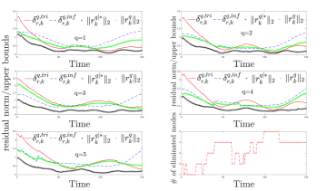
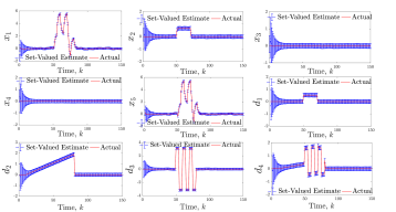
Refer to caption — Figure 1: $\|r^{q}_{r,k}\|_{2}$ , $\|r^{q|*}_{r,k}\|_{2}$ and their upper bounds for different modes, as well as the number of eliminated modes in time

Moreover, for each specific mode $q$ , the signals $\|r^{q}_{k}\|_{2},\|r^{q|*}_{k}\|_{2},\delta^{q,tri}_{r,k}$ and $\delta^{q,inf}_{r,k}$ are depicted in Figure 2. As can be seen, up to some large enough time, at different time intervals for different modes, one of the upper bounds may be tighter than the other, or vice-versa, so it is reasonable that we consider a minimum of them as the computed upper bound in our mode elimination algorithm. Furthermore, for all modes, $\delta^{q,tri}_{r,k}$ is eventually convergent while $\delta^{q,inf}_{r,k}$ diverges, as we proved in Lemma 3. So, after some large enough time, $\delta^{q,tri}_{r,k}$ can be used as our upper-bound, while $\delta^{q,inf}_{r,k}$ becomes useless. The corresponding set-valued estimates are provided in Figure 2.

VI Conclusion

We proposed a residual-based approach for hidden mode switched linear systems with bounded-norm noise and unknown attack signals . The proposed approach at each time step, removes the inconsistent modes and their corresponding observers from a bank of estimators, which includes mode-matched observers . Each mode-matched observer, conditioned on its corresponding mode being true, simultaneously finds bounded sets of states and unknown inputs that include the true state and inputs. Our mode elimination criterion required a bounded upper bound for the residual’s norm, for which we proved its existence and computed it by over-approximating the value function of a non-concave NP-hard norm-maximization problem by expanding its constraint set and converting it into a convex maximization over a convex set with finite number of extreme points. Such a problem can be solved by enumerating the objective function on the extreme points of the constraint set and comparing the corresponding values. Moreover, we proved the convergence of the upper bound signal and derived sufficient conditions for eventually eliminating all false modes using our mode elimination algorithm. Finally, we demonstrated the effectiveness of our observer using an illustrative example.

References

[1] A.A. Cárdenas, S. Amin, and S. Sastry. Research challenges for the security of control systems. In Proceedings of the 3rd Conference on Hot Topics in Security, HOTSEC’08, pages 6:1–6:6, 2008.
[2] K. Zetter. Inside the cunning, unprecedented hack of Ukraine’s power grid. Wired Magazine, 2016.
[3] H. Fawzi, P. Tabuada, and S. Diggavi. Secure estimation and control for cyber-physical systems under adversarial attacks. IEEE Transactions on Automatic control, 59(6):1454–1467, 2014.
[4] F. Pasqualetti, F. Dörfler, and F. Bullo. Attack detection and identification in cyber-physical systems. IEEE Transactions on Automatic Control, 58(11):2715–2729, November 2013.
[5] M. Pajic, J. Weimer, N. Bezzo, O. Sokolsky, G.J Pappas, and I. Lee. Design and implementation of attack-resilient cyberphysical systems: With a focus on attack-resilient state estimators. IEEE Control Systems Magazine, 37(2):66–81, 2017.
[6] S.Z. Yong, M. Zhu, and E. Frazzoli. Switching and data injection attacks on stochastic cyber-physical systems: Modeling, resilient estimation, and attack mitigation. ACM Transactions on Cyber-Physical Systems, 2(2):9, 2018.
[7] M.S Chong, M. Wakaiki, and J.P Hespanha. Observability of linear systems under adversarial attacks. In 2015 American Control Conference (ACC), pages 2439–2444. IEEE, 2015.
[8] Y. Shoukry and P. Tabuada. Event-triggered state observers for sparse sensor noise/attacks. IEEE Transactions on Automatic Control, 61(8):2079–2091, 2016.
[9] Y. Mo and E. Garone. Secure dynamic state estimation via local estimators. In 2016 IEEE 55th Conference on Decision and Control (CDC), pages 5073–5078. IEEE, 2016.
[10] W. Liu and I. Hwang. Robust estimation and fault detection and isolation algorithms for stochastic linear hybrid systems with unknown fault input. IET Control Theory Applications, 5(12):1353–1368, 2011.
[11] Y. Bar-Shalom, T. Kirubarajan, and X.R. Li. Estimation with Applications to Tracking and Navigation. John Wiley & Sons, Inc., New York, NY, USA, 2002.
[12] E. Mazor, A. Averbuch, Y. Bar-Shalom, and J. Dayan. Interacting multiple model methods in target tracking: a survey. IEEE Transactions on Aerospace and Electronic Systems, 34(1):103–123, Jan 1998.
[13] M.A Dahleh and I.J Diaz-Bobillo. Control of uncertain systems: a linear programming approach. Prentice-Hall, Inc., 1994.
[14] J.S. Shamma and K. Tu. Set-valued observers and optimal disturbance rejection. IEEE Trans. on Automatic Control, 44(2):253–264, 1999.
[15] F. Blanchini and M. Sznaier. A convex optimization approach to synthesizing bounded complexity $\ell^{\infty}$ filters. IEEE Transactions on Automatic Control, 57(1):216–221, 2012.
[16] S.Z. Yong. Simultaneous input and state set-valued observers with applications to attack-resilient estimation. In 2018 Annual American Control Conference (ACC), pages 5167–5174. IEEE, 2018.
[17] M. Khajenejad and S.Z. Yong. Simultaneous input and state set-valued $\mathcal{H}_{\infty}$ -observers for linear parameter-varying systems. In American Control Conference, pages 4521–4526, July 2019.
[18] R.J. Patton, P.M. Frank, and R.N. Clark. Issues of fault diagnosis for dynamic systems. Springer Science & Business Media, 2013.
[19] Y. Nakahira and Y. Mo. Attack-resilient $\mathcal{H}_{2}$ , $\mathcal{H}_{\infty}$ , and $\ell_{1}$ state estimator. arXiv preprint arXiv:1803.07053, 2018.
[20] D.P. Bertsekas, A. Nedich, A.E Ozdaglar, et al. Convex analysis and optimization. 2003.
[21] H.L. Bodlaender, P. Gritzmann, V. Klee, and J. Van Leeuwen. Computational complexity of norm-maximization. Combinatorica, 10(2):203–225, 1990.
[22] R.T. Rockafellar. Convex analysis. Princeton university press, 2015.
[23] J.F. Grcar. A matrix lower bound. Linear Algebra and its Applications, 433(1):203–220, 2010.

Appendix: Proofs

Proof of Lemma 3.

To show (18), we first find a lower bound for $\delta^{q,inf}_{r,k}$ . Then, we show that the lower bound diverges and so does $\delta^{q,inf}_{r,k}$ . Define $\tilde{t}^{\star}_{k}\triangleq{t^{\star}_{k}}/{\eta^{t}_{k}}$ , where $\eta^{t}_{k}$ is defined in Corollary 1. Now consider

	$\displaystyle\eta^{t}_{k}\sigma_{min}(\mathbb{A}^{q}_{k})$	$\displaystyle=\sigma_{min}(\eta^{t}_{k}\mathbb{A}^{q}_{k})=\min\limits_{\\|t\\|_{2}\leq 1}\\|\eta^{t}_{k}\mathbb{A}^{q}_{k}t\\|_{2}$
		$\displaystyle\leq\\|\eta^{t}_{k}\mathbb{A}^{q}_{k}\tilde{t}^{\star}_{k}\\|_{2}=\\|\mathbb{A}^{q}_{k}t^{\star}_{k}\\|_{2}=\delta^{q,inf}_{r,k},$

where $\sigma_{min}(A)$ is the least non-trivial singular value of matrix $A$ , the first equality holds since $\sigma_{min}(.)$ is a linear operator, the second equality is a special case of a matrix lower bound [23] when 2-norms are considered, the inequality holds since $\|\tilde{t}^{\star}_{k}\|_{2}=1$ by Corollary 1, so $\tilde{t}^{\star}_{k}$ is a feasible point for the minimization in the third statement and the last equality holds by Theorem 3. So far we have shown that $\eta^{t}_{k}\sigma_{min}(\mathbb{A}^{q}_{k})$ is a lower bound for $\delta^{q,inf}_{r,k}$ . Next, we will prove that $\eta^{t}_{k}\sigma_{min}(\mathbb{A}^{q}_{k})$ is unbounded. First, it is trivial that $\eta^{t}_{k}$ is unbounded by its definition in Corollary 1. Second, consider the block matrix $\mathbb{A}^{q}_{k}$ in Lemma 1. By the strong detectability assumption, matrix $A^{q}_{e}$ is stable [16, Theorem 3 and Appendix C], so all the block matrices of $\mathbb{A}^{q}_{k}$ , except three of them which are constant matrices with respect to time, converge to zero matrices when time goes to infinity. Hence $\mathbb{A}^{q}_{k}$ converges to an infinite dimensional sparse matrix, with only three non-zero finite dimensional constant blocks and so the limit matrix has a finite rank and clearly has a bounded minimum non-trivial singular value. Henceforth, $\eta^{t}_{k}\sigma_{min}(\mathbb{A}^{q}_{k})$ is unbounded, since the product of the bounded and non-zero $\sigma_{min}(\mathbb{A}^{q}_{k})$ and unbounded $\eta^{t}_{k}$ is unbounded. As for (19), the first equality holds by definition of $\hat{\delta}^{q}_{r,k}$ ( cf. Theorem 3) and (18), the first inequality holds since $\delta^{q,tri}_{r,k}\leq\overline{\delta}^{q,r}_{r,k}$ by triangle and sub-multiplicative inequalities and the last equality, i.e., convergence of $\delta^{q,tri}_{r,k}$ , follows from strong detectability assumption which implies the stability of ${A^{q}_{e}}$ [16, Theorem 3].∎

Proof of Lemma 4.

Suppose, for contradiction, that none of $q$ and $q^{\prime}$ are eliminated. Then

	$\displaystyle\\|C^{q}_{2}\hat{x}^{\star,q}_{k\|k}+D^{q}_{2}u^{q}_{k}-C^{q^{\prime}}_{2}\hat{x}^{\star,q^{\prime}}_{k\|k}-D^{q^{\prime}}_{2}u^{q^{\prime}}_{k}\\|_{2}=$
	$\displaystyle\\|r^{q^{\prime}}_{k}-r^{q}_{k}+z^{q}_{2,k}-z^{q^{\prime}}_{2,k})\\|_{2}\leq\\|r^{q^{\prime}}_{k}\\|_{2}+\\|r^{q}_{k}\\|_{2}+\\|z^{q}_{2,k}-z^{q^{\prime}}_{2,k}\\|_{2}$
	$\displaystyle\leq\delta^{q}_{r,k}+\delta^{q^{\prime}}_{r,k}+R_{y}\\|T^{q}_{2}-T^{q^{\prime}}_{2}\\|_{2},$

where the equality holds by Definition 1, the first inequality holds by triangle inequality and the last inequality holds by the assumption that none of $q$ and $q^{\prime}$ can be eliminated, as well as the boundedness assumption for the measurement space. This last inequality contradicts with the inequality in the lemma, thus the result holds. ∎

Proof of Lemma 5.

The result can be obtained by applying Proposition 1, (14) and the closed-form output signal:

\displaystyle y_{k}

\displaystyle=\begin{bmatrix}\begin{bmatrix}(CA^{k})^{\top}\\ (CA^{k-1})^{\top}\\ \vdots\\ C^{\top}\\ I\end{bmatrix}^{\top}&\begin{bmatrix}H^{\top}\\ (CG)^{\top}\\ (CAG)^{\top}\\ \vdots\\ (CA^{k-1}G)^{\top}\end{bmatrix}^{\top}&\begin{bmatrix}D^{\top}\\ (CB)^{\top}\\ (CAB)^{\top}\\ \vdots\\ (CA^{k-1}B)^{\top}\end{bmatrix}^{\top}\end{bmatrix}\begin{bmatrix}t_{k}\\[-5.69046pt] \\ d^{q*}_{0:k}\\[-5.69046pt] \\ u^{q*}_{0:k}\end{bmatrix},

which can be derived by using (3) and simple induction. ∎

Proof of Theorem 4.

To show that (i) is sufficient for asymptotic mode detectability, consider Lemma 4 with $\delta^{q,tri}_{r,k}$ as the upper bound. It suffices to show $\exists K\in\mathbb{N}$ , such that (20) holds for $k\geq K,\forall q\neq q^{\prime}\in\mathbb{Q}.$ Notice that by Definition 1, $C^{q}_{2}\hat{x}^{\star,q}_{k|k}=C^{q}_{2}x_{k}+T^{q}_{2}v_{k}-r^{q|*}_{k}$ . Plugging this into (20), we need to show $\exists K\in\mathbb{N}$ such that:

	$\displaystyle\\|W^{q,q^{\prime}}s^{q,q^{\prime}}_{k}\\|_{2}>\delta^{q,tri}_{r,k}+\delta^{q^{\prime},tri}_{r,k}+R^{q,q^{\prime}}_{z},\forall k\geq K,$		(21)
	$\displaystyle s^{q,q^{\prime}}_{k}\triangleq\begin{bmatrix}x^{\top}_{k}&v^{\top}_{k}&r^{q\|\top}_{k}&r^{q^{\prime}\|\top}_{k}&u^{q\top}_{k}&u^{q^{\prime}\top}_{k}\end{bmatrix}^{\top},\forall q\neq q^{\prime}\in\mathbb{Q}.$

A sufficient condition to satisfy (21) is that $\exists K\in\mathbb{N}$ such that $\forall k\geq K$ , (21) holds for all $s^{q,q^{\prime}}_{k}$ . Equivalently, it suffices

	$\displaystyle\min\limits_{x_{k},v_{k},r^{q}_{k},r^{q^{\prime}}_{k}}\\|W^{q,q^{\prime}}s^{q,q^{\prime}}_{k}\\|_{2}>\delta^{q,tri}_{r,k}+\delta^{q^{\prime},tri}_{r,k}+R^{q,q^{\prime}}_{z}$
	$\displaystyle s.t.\ \\|x_{k}\\|_{2}\leq R_{x},\\|v_{k}\\|_{2}\leq\eta_{v},\\|r^{q\|*}_{k}\\|_{2}\leq\delta^{q,tri}_{r,k},$
	$\displaystyle\ \ \ \ \ \\|r^{q^{\prime}\|*}_{k}\\|_{2}\leq\delta^{q^{\prime},tri}_{r,k},\ \forall k\geq K,\forall q\neq q^{\prime}\in\mathbb{Q}.$

By expanding the constraint set, it is sufficient to require that $\exists K\in\mathbb{N}$ such that:

		$\displaystyle\min\limits_{s^{q,q^{\prime}}_{k}}\\|W^{q,q^{\prime}}s^{q,q^{\prime}}_{k}\\|_{2}>\delta^{q,tri}_{r,k}+\delta^{q^{\prime},tri}_{r,k}+R^{q,q^{\prime}}_{z}$
	$\displaystyle s.t.\$	$\displaystyle\\|s^{q,q^{\prime}}_{k}\\|^{2}_{2}\leq R^{2}_{x}+\eta^{2}_{v}+(\delta^{q,tri}_{r,k})^{2}+(\delta^{q^{\prime},tri}_{r,k})^{2}+(u^{q}_{k})^{2}+(u^{q^{\prime}}_{k})^{2}$
		$\displaystyle\forall k\geq K,\forall q\neq q^{\prime}\in\mathbb{Q}.$

Now, by matrix lower bound theorem [23] and similar argument as in the proof of Lemma 3, it is sufficient to be satisfied that $\exists K\in\mathbb{N}\ s.t.\ \forall k\geq K,\forall q\neq q^{\prime}\in\mathbb{Q}:$

\displaystyle\sigma^{2}_{min}(W^{q,q^{\prime}})>\frac{(\delta^{q,tri}_{r,k}+\delta^{q^{\prime},tri}_{r,k}+R^{q,q^{\prime}}_{z})^{2}}{R^{2}_{x}+\eta^{2}_{v}+(\delta^{q,tri}_{r,k})^{2}+(\delta^{q^{\prime},tri}_{r,k})^{2}+(u^{q}_{k})^{2}+(u^{q^{\prime}}_{k})^{2}}.

(22)

(22) provides us a time-dependent sufficient condition for mode detectability. In order to find a time-independent sufficient condition, notice that $\frac{(\overline{\delta}^{q,tri}_{r,k}+\overline{\delta}^{q^{\prime},tri}_{r,k}+R^{q,q^{\prime}}_{z})^{2}}{R^{2}_{x}+\eta^{2}_{v}}$ is an upper bound for the right hand side of (22), since the latter’s denominator is smaller than the former’s and the numerator of the latter is an upper bound signal for the former’s by triangle and sub-multiplicative inequalities. So a sufficient condition for (22) is $\exists K\in\mathbb{N}\ s.t.\ \forall k\geq K,\forall q\neq q^{\prime}\in\mathbb{Q}:$

\displaystyle\sigma^{2}_{min}(W^{q,q^{\prime}})>\frac{(\overline{\delta}^{q,tri}_{r,k}+\overline{\delta}^{q^{\prime},tri}_{r,k}+R^{q,q^{\prime}}_{z})^{2}}{R^{2}_{x}+\eta^{2}_{v}}.

(23)

Then, for the above to hold, it suffices that

\sigma^{2}_{min}(W^{q,q^{\prime}})>\lim_{k\to\infty}\frac{(\overline{\delta}^{q,tri}_{r,k}+\overline{\delta}^{q^{\prime},tri}_{r,k}+R^{q,q^{\prime}}_{z})^{2}}{R^{2}_{x}+\eta^{2}_{v}},

which is equivalent to (i) by (19). As for the sufficiency of (ii), notice that by Theorems 2 and 3, Lemma 1 and Definition 2, for mode detectability, it suffices that for any specific mode $q$ , the true mode $q^{*}$ and large enough $k$ ,

\displaystyle\|r^{q}_{k}\|_{2}=\|\begin{bmatrix}\mathbb{T}^{q,q^{*}}_{k}&\mathbb{B}^{q,q^{*}}_{k}&\mathbb{D}^{q,q^{*}}_{k}\end{bmatrix}\begin{bmatrix}t^{\top}_{k}&u^{q^{*}\top}_{0:k}&d^{q*\top}_{0:k}\end{bmatrix}^{\top}\|_{2}>\delta^{q,tri}_{r,k},

with $t_{k}$ given in (17). Since $q^{*}$ is unknown, a sufficient condition to satisfy the above equality is $\forall q^{\prime}\neq q\in Q:$

\displaystyle\|r^{q}_{k}\|_{2}=\|\begin{bmatrix}\mathbb{T}^{q,q^{\prime}}_{k}&\mathbb{B}^{q,q^{\prime}}_{k}&\mathbb{D}^{q,q^{\prime}}_{k}\end{bmatrix}\begin{bmatrix}t^{\top}_{k}&u^{q^{\prime}\top}_{0:k}&d^{q*\top}_{0:k}\end{bmatrix}^{\top}\|_{2}>\delta^{q,tri}_{r,k}.

So it suffices that $\forall q^{\prime}\neq q\in Q,\exists\overline{d}\in\mathbb{R}$ , such that:

	$\displaystyle\min\limits_{t^{\prime}_{k}}\\|\begin{bmatrix}\mathbb{T}^{q,q^{\prime}}_{k}&\mathbb{B}^{q,q^{\prime}}_{k}&\mathbb{D}^{q,q^{\prime}}_{k}\end{bmatrix}{\color[rgb]{0,0,0}t^{\prime}_{k}}\\|_{2}>\delta^{q,tri}_{r,k}$
	$\displaystyle s.t.\ t^{\prime}_{k}=\begin{bmatrix}t^{\top}_{k}&u^{q^{\prime}\top}_{0:k}&d^{q\top}_{0:k}\end{bmatrix}^{\top},\\|d^{q}_{0:k}\\|_{2}\geq\overline{d},$
	$\displaystyle\ \ \ \ \ t_{k}=\begin{bmatrix}\tilde{x}^{\top}_{0\|0}&w^{\top}_{0}&\dots&w^{\top}_{k-1}&v^{\top}_{0}&\dots&v^{\top}_{k}\end{bmatrix},$
	$\displaystyle\ \ \ \ \ \\|\tilde{x}_{0\|0}\\|_{\infty}\leq\delta^{x}_{0},\ \\|w_{i}\\|_{\infty}\leq\eta_{w},\ \\|v_{j}\\|_{\infty}\leq\eta_{v},$
	$\displaystyle\ \ \ \ \ \forall i\in\{0,...,k-1\},\ \forall j\in\{0,...,k\}{\color[rgb]{0,0,0}.}$

Again by matrix lower bound theorem, a sufficient condition for the above inequality to hold is that $\exists\overline{d}\in\mathbb{R}$ , such that:

		$\displaystyle\min\limits_{t_{k},d_{0:k}}\\|t^{\prime}_{k}\\|_{2}>\frac{{\delta}^{q,tri}_{r,k}}{\sigma_{min}\begin{bmatrix}\mathbb{T}^{q,q^{\prime}}_{k}&\mathbb{B}^{q,q^{\prime}}_{k}&\mathbb{D}^{q,q^{\prime}}_{k}\end{bmatrix}}$		(24)
		$\displaystyle s.t.\ t^{\prime}_{k}=\begin{bmatrix}t^{\top}_{k}&u^{q^{\prime}\top}_{0:k}&d^{q\top}_{0:k}\end{bmatrix}^{\top},\\|d^{q}_{0:k}\\|_{2}\geq\overline{d},$
		$\displaystyle\ \ \ \ \ t_{k}=\begin{bmatrix}\tilde{x}^{\top}_{0\|0}&w^{\top}_{0}&\dots&w^{\top}_{k-1}&v^{\top}_{0}&\dots&v^{\top}_{k}\end{bmatrix},$
		$\displaystyle\ \ \ \ \ \\|\tilde{x}_{0\|0}\\|_{\infty}\leq\delta^{x}_{0},\ \\|w_{i}\\|_{\infty}\leq\eta_{w},\ \\|v_{j}\\|_{\infty}\leq\eta_{v},$
		$\displaystyle\ \ \ \ \ \forall i\in\{0,...,k-1\},\ \forall j\in\{0,...,k\}.$

Finally, since ${\delta}^{q,tri}_{r,k}\leq\overline{\delta}^{q,tri}_{r,k}$ and

\displaystyle\|t^{\prime}_{k}\|_{2}=\|\begin{bmatrix}t^{\top}_{k}&u^{q^{\prime}\top}_{0:k}&d^{q*\top}_{0:k}\end{bmatrix}\|_{2}\geq\sqrt{0^{2}+0^{2}+\|d^{q*\top}_{0:k}\|^{2}_{2}}=\|d^{q*\top}_{0:k}\|_{2},

then a sufficient condition for (24) is that

\displaystyle\|d^{q*\top}_{0:k}\|_{2}>\frac{\overline{\delta}^{q,tri}_{r,k}}{\sigma_{min}{\color[rgb]{0,0,0}(}\begin{bmatrix}\mathbb{T}^{q,q^{\prime}}_{k}&\mathbb{B}^{q,q^{\prime}}_{k}&\mathbb{D}^{q,q^{\prime}}_{k}\end{bmatrix}{\color[rgb]{0,0,0})}}.

(25)

Now suppose that $T^{q}_{2}\neq T^{q^{\prime}}_{2}$ (otherwise the matrix in the denominator of (25) is zero and it never holds). Asymptotically speaking, the right hand side of (25) converges to $\tilde{\delta}\triangleq\max\{0,(\overline{\delta}^{q,tri}_{r}/\overline{\sigma}^{q,q^{\prime}})\}$ , since $\overline{\delta}^{q,tri}_{r,k}$ converges to $\overline{\delta}^{q,tri}_{r}$ and the least singular value in the denominator either diverges or converges to some steady value $\overline{\sigma}^{q,q^{\prime}}$ . So we set $\overline{d}$ equal to any real number strictly grater than $\tilde{\delta}$ . By unlimited energy assumption for attack signal, after some large enough time step $K$ , the monotone increasing function $\|d^{q*}_{0:k}\|_{2}$ , exceeds $\overline{d}$ and so the system will be mode detectable. ∎

		$\displaystyle\delta^{q}_{r,k}\triangleq\max\limits_{t_{k}}\\|\mathbb{A}^{q}_{k}{t}_{k}\\|_{2}$		(16)
		$\displaystyle s.t.\ t_{k}=\begin{bmatrix}\tilde{x}^{\top}_{0\|0}&w^{\top}_{0}&\dots&w^{\top}_{k-1}&v^{\top}_{0}&\dots&v^{\top}_{k}\end{bmatrix}^{\top},$
		$\displaystyle\\|\tilde{x}_{0\|0}\\|_{2}\leq\delta^{x}_{0},\ \\|w_{i}\\|_{2}\leq\eta_{w},\ \\|v_{j}\\|_{2}\leq\eta_{v},$
		$\displaystyle i\in\{0,...,k-1\},\ j\in\{0,...,k\}.$

	$\displaystyle\hat{\delta}^{q}_{r,k}\triangleq\min\{\delta^{q,inf}_{r,k},{\delta}^{q,tri}_{r,k}\},$
	$\displaystyle\delta^{q,inf}_{r,k}\triangleq\\|\mathbb{A}^{q}_{k}{t}^{\star}_{k}\\|_{2},$
	$\displaystyle\delta^{q,tri}_{r,k}\triangleq\delta^{x,q}_{0}\\|C^{q}_{2}\overline{A}^{q}{A^{q}_{e}}^{k-1}\\|_{2}+\eta_{w}\\|C^{q}_{2}\overline{A}^{q}{A^{q}_{e}}^{k-2}\\|_{2}+$
	$\displaystyle\ \ \textstyle\sum_{i=1}^{k-2}[\eta_{w}\\|C^{q}_{2}\overline{A}^{q}{A^{q}_{e}}^{i}B^{q}_{e,w}\\|_{2}+\eta_{v}\\|C^{q}_{2}\overline{A}^{q}{A^{q}_{e}}^{i}(B^{q}_{e,v_{1}}+{A^{q}_{e}}B^{q}_{e,v_{2}})\\|_{2}]$
	$\displaystyle\quad+\eta_{v}(\\|C^{q}_{2}\overline{A}^{q}{A^{q}_{e}}^{k-2}B^{q}_{e,v_{1}}\\|_{2}+\\|C^{q}_{2}(B^{q,\star}_{e,v_{1}}+\overline{A}^{q}B^{q}_{e,v_{2}})\\|_{2})$
	$\displaystyle\quad+\\|C^{q}_{2}B^{q,\star}_{e,v_{2}}+T^{q}_{2}\\|_{2})+\eta_{w}\\|C^{q}_{2}B^{\star,q}_{e,w}\\|_{2},$

	$\displaystyle\delta^{q,inf}_{r,k}\triangleq\max\limits_{t_{k}}\\|\mathbb{A}^{q}_{k}{t}_{k}\\|_{2}$		(17)
	$\displaystyle s.t.\ t_{k}=\begin{bmatrix}\tilde{x}^{\top}_{0\|0}&w^{\top}_{0}&\dots&w^{\top}_{k-1}&v^{\top}_{0}&\dots&v^{\top}_{k}\end{bmatrix},$
	$\displaystyle\ \ \ \ \ \\|\tilde{x}_{0\|0}\\|_{\infty}\leq\delta^{x}_{0},\ \\|w_{i}\\|_{\infty}\leq\eta_{w},\ \\|v_{j}\\|_{\infty}\leq\eta_{v},$
	$\displaystyle\ \ \ \ \ \forall i\in\{0,...,k-1\},\ \forall j\in\{0,...,k\}.$

	$\displaystyle\min\limits_{t^{\prime}_{k}}\\|\begin{bmatrix}\mathbb{T}^{q,q^{\prime}}_{k}&\mathbb{B}^{q,q^{\prime}}_{k}&\mathbb{D}^{q,q^{\prime}}_{k}\end{bmatrix}{\color[rgb]{0,0,0}t^{\prime}_{k}}\\|_{2}>\delta^{q,tri}_{r,k}$
	$\displaystyle s.t.\ t^{\prime}_{k}=\begin{bmatrix}t^{\top}_{k}&u^{q^{\prime}\top}_{0:k}&d^{q\top}_{0:k}\end{bmatrix}^{\top},\\|d^{q}_{0:k}\\|_{2}\geq\overline{d},$
	$\displaystyle\ \ \ \ \ t_{k}=\begin{bmatrix}\tilde{x}^{\top}_{0\|0}&w^{\top}_{0}&\dots&w^{\top}_{k-1}&v^{\top}_{0}&\dots&v^{\top}_{k}\end{bmatrix},$
	$\displaystyle\ \ \ \ \ \\|\tilde{x}_{0\|0}\\|_{\infty}\leq\delta^{x}_{0},\ \\|w_{i}\\|_{\infty}\leq\eta_{w},\ \\|v_{j}\\|_{\infty}\leq\eta_{v},$
	$\displaystyle\ \ \ \ \ \forall i\in\{0,...,k-1\},\ \forall j\in\{0,...,k\}{\color[rgb]{0,0,0}.}$

		$\displaystyle\min\limits_{t_{k},d_{0:k}}\\|t^{\prime}_{k}\\|_{2}>\frac{{\delta}^{q,tri}_{r,k}}{\sigma_{min}\begin{bmatrix}\mathbb{T}^{q,q^{\prime}}_{k}&\mathbb{B}^{q,q^{\prime}}_{k}&\mathbb{D}^{q,q^{\prime}}_{k}\end{bmatrix}}$		(24)
		$\displaystyle s.t.\ t^{\prime}_{k}=\begin{bmatrix}t^{\top}_{k}&u^{q^{\prime}\top}_{0:k}&d^{q\top}_{0:k}\end{bmatrix}^{\top},\\|d^{q}_{0:k}\\|_{2}\geq\overline{d},$
		$\displaystyle\ \ \ \ \ t_{k}=\begin{bmatrix}\tilde{x}^{\top}_{0\|0}&w^{\top}_{0}&\dots&w^{\top}_{k-1}&v^{\top}_{0}&\dots&v^{\top}_{k}\end{bmatrix},$
		$\displaystyle\ \ \ \ \ \\|\tilde{x}_{0\|0}\\|_{\infty}\leq\delta^{x}_{0},\ \\|w_{i}\\|_{\infty}\leq\eta_{w},\ \\|v_{j}\\|_{\infty}\leq\eta_{v},$
		$\displaystyle\ \ \ \ \ \forall i\in\{0,...,k-1\},\ \forall j\in\{0,...,k\}.$