Simultaneous Distributed Estimation and Attack Detection/Isolation in Social Networks: Structural Observability, Kronecker-Product Network, and Chi-Square Detector

The unprecedented large size of social networks mandates distributed sensing, inference, and detection [1, 2, 3, 4, 5, 6, 7], where the information is collected and processed locally while meeting certain security concerns. Recent distributed estimation protocols [6, 7, 8, 9, 10, 11] are prone to faults/attacks that may result in inaccurate state estimates. Different attack detection and FDI (fault detection and isolation) strategies are thus proposed in the literature, ranging in applications from biological modeling [12] to smart-grid monitoring [13, 14], and from centralized approaches [15, 16, 17, 18, 19, 20] to more recent distributed methods [21, 22, 23]. Among the centralized solutions, deterministic FDI and attack detection methods design decision thresholds based on the upper-bound on the noise support [17, 18], while, in contrast, probabilistic $\chi^{2}$-test with no such assumption on the noise is proposed in [15] and further developed in [19, 20]. Among the distributed strategies, [23] requires injecting a watermarking input signal conceding to a loss in the control/estimation performance, which is not applicable to autonomous systems (such as the social network model in this paper). In order to close this gap, this paper aims at developing a technique for distributed inference of autonomous (social) systems while simultaneously detecting and isolating adversarial attacks locally with no central coordinator.

The main contributions of this paper are as follows. (i) This work considers a windowed $\chi^{2}$ benchmark to locally design probabilistic decision thresholds based on certain false alarm rates (FARs). This is in contrast to existing deterministic thresholds assuming certain upper-bound on the noise support [17, 18], which results in faulty outcome when the noise upper-bound is considerably larger than the attack/fault magnitude. (ii) This work extends the recent centralized $\chi^{2}$ detectors [19, 20] to distributed ones, where the sensors are widespread over a large social network and, thus, the centralized solutions are infeasible/undesirable due to heavy communication loads or inability for parallel processing. In this direction, the notion of Kronecker-product network [24] is used to perceive (structural) observability of the composite social/sensor network, which allows to find minimal connectivity requirement on the sensor network for distributed estimation/detection. (iii) Our distributed technique, as in [21, 22], does not require local-observability at every sensor. However, unlike fixed biasing faults/attacks on sensor outputs in [21, 22], this work extends the results to general anomalies in the form of a random variable. In particular, we adopt the notion of distance measure [19], a scalar variable to compare the residual variance in presence and absence of attacks.

We consider the interaction of individuals in a social network as a linear-structure-invariant (LSI) autonomous model [4, 5, 7, 6],

where $k$ is the time-step, $A$ is the social system matrix associated with social digraph $\mathcal{G}$, $\nu_{k}\sim\mathcal{N}(0,Q)$ is additive i.i.d noise vector, and vector ${\mathbf{x}_{k}=\left[{x}_{k}^{1},\dots,{x}_{k}^{n}\right]^{\top}\in\mathbb{R}^{n}}$ represents the global social state. Note that $n$ is the size of social network and $\mathbf{x}_{k}^{i}$ represents the $i$’th individual’s social state, e.g., opinion, rumor, or attitude [1, 2, 3, 4, 6, 7, 5]. The state $\mathbf{x}_{k}^{i}$ of individual $i$ at time $k$ is a weighted average of the states $\mathbf{x}_{k-1}^{j}$ of its in-neighbors in $\mathcal{G}$ and its own previous state $\mathbf{x}_{k-1}^{i}$. This is well-justified for opinion-dynamics in social systems, and particularly implies that matrix $A$ is (structurally) full-rank [7]. Consider $N$ social sensors (agents or information-gatherers [5]) sensing the state of some individuals as,

with $H_{i}$ as the measurement matrix, $\tau_{k}^{i}$ as possible attack and $\eta_{k}^{i}\sim\mathcal{N}(0,R_{i})$ as Gaussian noise at sensor $i$ at time $k$. Define $R=\text{diag}[R_{i}]$ as the covariance matrix of the i.i.d noise vector $\eta_{k}$. Throughout this paper, without loss of generality, we assume every sensor observes one state variable, i.e., ${y}_{k}^{i}\in\mathbb{R}$. Further, as in similar works [15, 19, 20], we assume the system and measurement noise covariance ($Q$ and $R$) are known. Then, sensors share their information over a sensor network $\mathcal{G}_{N}$. Clearly, system $A$ is not locally observable to any sensor, but globally observable to all sensors. The condition on $(A,H)$-observability is given in the following lemma.

Given (social) system (1) and state observations (2) satisfying Lemma 1, we aim to design a distributed iterative procedure to simultaneously estimate the (social) state $\mathbf{x}_{k}^{i}$ while detecting adversary attacks at (social) sensors. The attack by the adversary is modeled as an additive random term $\tau_{k}^{i}$ at sensor $i$ in (2). The proposed distributed estimation makes the entire system observable to every sensor, and the attack-detection technique enables each sensor to locally detect anomalies in its observation with a certain FAR (false-alarm rate).

We consider a modified version of the single time-scale distributed estimator in [7] with one step of averaging on a-priori estimates (similar to DeGroot consensus model [8]) and one step of measurement update (also known as innovation [8]),

with stochastic matrix $W=\{w_{ij}\}$ as the adjacency matrix of the sensor network $\mathcal{G}_{N}$ representing the fusion weights among the sensors, $K_{i}$ as the local gain matrix at agent $i$, and $\widehat{\mathbf{x}}^{i}_{k|k-1}$ and $\widehat{\mathbf{x}}^{i}_{k|k}$ as the state estimate at time $k$ given all the information of agent $i$ and its in-neighbors $\mathcal{N}(i)$, respectively, at time $k-1$ and $k$. In contrast to double time-scale estimators/observers [11] with many consensus iterations between every two consecutive time-steps $k-1$ and $k$ of social dynamics (1), the estimator (3)-(4) performs one iteration of information fusion between steps $k-1$ and $k$, which is more efficient in terms of computation/communication loads.

Define the estimation error at agent $i$ as $\mathbf{e}_{k}^{i}=\mathbf{x}_{k}-\widehat{\mathbf{x}}^{i}_{k|k}$ and the error vector $\mathbf{e}_{k}=\left[(\mathbf{e}_{k}^{1})^{\top},\dots,(\mathbf{e}_{k}^{n})^{\top}\right]^{\top}$. Following similar procedure as in [6], the error dynamics is as follows,

with $D_{H}=\text{diag}[H_{i}^{\top}H_{i}]$, $K=\text{diag}[K_{i}]$ as the feedback gain matrix, and $\mathbf{q}_{k}$ as the collective vector of noise-related terms $\mathbf{q}_{k}=\left[(\mathbf{q}_{k}^{1})^{\top},\dots,(\mathbf{q}_{k}^{n})^{\top}\right]^{\top}$ as,

with $\mathbf{1}_{N}$ as the vector of $1$’s of size $N$ and $\overline{D}_{H}=\mbox{diag}[H_{i}^{\top}]$. Following Kalman theory, for bounded steady-state estimation error, $(W\otimes A,D_{H})$ needs to be observable, characterizing the distributed observability condition for network of estimators/observers [25]. Using structured system theory, this condition can be investigated via graph theoretic notions. In this direction, the associated network to $W\otimes A$ is a Kronecker-product network, whose observability condition relies on the structure of both $\mathcal{G}$ and $\mathcal{G}_{N}$. Given the social network $\mathcal{G}$, the conditions on the sensor network $\mathcal{G}_{N}$ to satisfy distributed observability follows the recent results on composite-network theory and network observability discussed in [24], which is summarized in the following lemma.

For an observable pair $(W\otimes A,D_{H})$, the feedback gain matrix $K$ can be designed to stabilize the error dynamics (5). Mathematically, for $\overline{A}=W\otimes A-KD_{H}(W\otimes A)$, we need to design $K$ such that $\rho(\overline{A})<1$ (Schur stability of error dynamics (5)) for general social systems with $\rho(A)>1$ with $\rho(\cdot)$ as the spectral radius. As mentioned before, for distributed case, $K$ needs to be further block-diagonal such that each sensor only uses local information in its own neighborhood. The iterative LMI-based algorithm to design such block-diagonal gain $K$ is given in [26]. In attack-free scenario, the distributed estimator/observer (3)-(4) with proper gain $K$ ensures tracking the global social state with bounded steady-state error as discussed in [6, 7]. Next, in this section, we further study the performance of the proposed protocol in the presence of non-zero random attack signals. Define $\widehat{y}_{k}^{i}=H_{i}\widehat{\mathbf{x}}_{k|k}^{i}$ as the estimated output at sensor $i$ at time $k$. To detect possible attacks, each sensor calculates its residual as the difference of its original output and the estimated one,

Having $\rho(\overline{A})<1$, the steady-state error in (5) only relies on the term $\mathbf{q}_{k}^{i}$ defined in (6) as,

From (8) and (9), it is clear that for $\mathbf{\tau}^{i}_{k}\neq 0$, only the residual $r_{k}^{i}$ at sensor $i$ is biased with no effect on the residual of other sensors $j\neq i$. This allows to isolate the attacked sensor as $r_{k}^{i}$ only depends on $\mathbf{\tau}^{i}_{k}$ and not on $\mathbf{\tau}^{j}_{k}$’s. To detect a possible attack at agent $i$ via residual $r_{k}^{i}$, the non-zero term $\mathbf{\tau}^{i}_{k}-H_{i}K_{i}H_{i}^{\top}\mathbf{\tau}_{k}^{i}$ needs to be sufficiently larger than other noise terms. This ensures that the residual in attacked case is large enough to be distinguished from the noise terms in attack-free case. This is done by adding the constraint $|1-H_{i}K_{i}H_{i}^{\top}|>C$ (with $C$ as a pre-selected lower-bound) to the proposed LMI in [26]. To the best of our knowledge, no other analytical solution for such constrained design is given in the literature. Clearly, the detecting probability of an attack depends on the magnitude of $\mathbf{\tau}^{i}_{k}$, which justifies the probabilistic threshold design. In this direction, we consider a distributed probability-based $\chi^{2}$-test which outperforms the deterministic fault/attack detection methods as it considers noise of unbounded support. In this case, instead of a deterministic threshold with $0$ (no attack) or $1$ (attack detected) outcome, different probabilistic thresholds (with different sensitivities) are defined each assigned with an FAR. In fact, higher residual-to-noise ratio (RNR) stimulates the threshold with lower FAR. In this direction, first the covariance of error $\mathbf{e}_{k}$ and (attack-free) residuals need to be calculated, which are tied with the noise covariance $Q$ and $R$. Let $\Xi_{k}=\mathbb{E}(\mathbf{e}_{k}\mathbf{e}_{k}^{\top})$ and $\Sigma=\mathbb{E}(\mathbf{q}_{k}\mathbf{q}^{\top}_{k})$. Then, from (5),

Knowing that $\rho(\overline{A})<1$, the first term in (10) goes to zero. Therefore, it can be proved from [4] that for $\Xi_{\infty}=\lim_{k\rightarrow\infty}\Xi_{k}$,

with $b=\|\overline{A}\|_{2}<1$. For attack-free case ($\mathbf{\tau}_{k}=\mathbf{0}_{N}$ in (6)),

where $\mathbf{1}_{NN}$ is the $1$’s matrix of size $N$. Applying the $\mathbb{E}(\cdot)$ and $2$-norm operators,

Then, the upper-bound on $\|\Sigma\|_{2}$ is,

with $\overline{R}=\mbox{diag}[H_{i}^{\top}R_{i}H_{i}]$. Then, using (11),

where $\|I_{Nn}-KD_{H}\|_{2}^{2}=a_{1}$, $\|K\|_{2}^{2}=a_{2}$, and $\|\overline{R}\|_{2}=a_{3}\|R\|_{2}$. Note that in (14) the error covariance is scaled by the number of sensors $N$. From (14), assuming no attack is present ($\mathbf{\tau}_{k}^{i}=0$), a conservative approximation for error variance at sensor $i$ is $\mathbb{E}((\mathbf{e}^{i}_{k})(\mathbf{e}_{k}^{i})^{\top})=\Phi$. Then, following the discussion in [19], the residual $r^{i}_{k}$ in (8) can be assumed as a zero-mean Gaussian variable with maximum variance ${\Lambda_{i}=\mathbb{E}((r^{i}_{k})(r_{k}^{i})^{\top})=H_{i}^{\top}\Phi H_{i}+R_{i}}$, i.e., $r_{k}^{i}\sim\mathcal{N}(0,\Lambda_{i})$. Define,

with $T$ as the length of the sliding window¹¹1In general, each agent can consider a different length for the horizon T.. It is known that, for a Gaussian variable $r_{k}^{i}$, scalars $z_{k}^{i}$ and $v_{k}^{i}$ follow $\chi_{1}^{2}$-distribution with degree $1$ and $T$ respectively ($\mathbb{E}[z_{k}^{i}]=1$ and $\mathbb{E}[v_{k}^{i}]=T$) [27]. In fact, these so-called distance measures $z_{k}^{i}$ and $v_{k}^{i}$ give an estimate of variance of $r_{k}^{i}$ relative to the attack-free variance $\Lambda_{i}$ [19], and are known to outperform simple detectors comparing absolute residual to a threshold as in [21, 22]. Next, we determine the decision threshold $\theta$ on $v_{k}^{i}$ based on a pre-specified FAR $p$. It can be shown that $p=1-F(\theta)$ where $F(\cdot)$ is the cumulative distribution function (CDF) of $\chi_{1}^{2}$-distribution. Then,

with $\Gamma^{-1}(\cdot,\cdot)$ as the inverse regularized lower incomplete gamma function [27]. Using (16), our attack detection logic at each sensor $i$ is as follows,

It should be noted that the existing $\chi^{2}$-based attack detection scenarios in literature are all centralized [15, 19, 20] and in this work, using distributed estimation, we enable detection of attacks locally at every sensor with no need of a central unit. We summarize our proposed simultaneous distributed estimation and attack detection technique in Algorithm 1.

Note that after detecting a malicious attack with low FAR, the strategy in [28] can be adopted to remove unreliable data and replace the compromised sensor with its observationally equivalent counterpart to regain distributed observability.

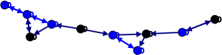
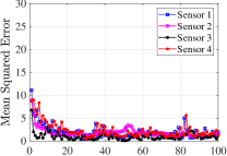
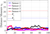
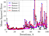
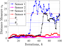
We evaluate our theoretical results on an example social network $\mathcal{G}$ of $10$ state nodes with $4$ sensor observations shown in Fig. 1. The network $\mathcal{G}_{N}$ of $4$ sensors is considered as a cycle (satisfying Lemma 2). The fixed non-zero entries of $A$ and $W$ are chosen randomly in $(0,1.1]$. Further, $\rho(A)=1.1$ implying a potentially unstable system, $\eta_{k}^{i},\nu_{k}^{i}\sim\mathcal{N}(0,0.06)$, and non-zero entries of $H$ are set as $1$. Using MATLAB’s CVX, the stabilizing block-diagonal gain $K$ is designed via the iterative LMI in [26] subject to $|1-H_{i}K_{i}H_{i}^{\top}|>0.2$, which results in $\rho(\overline{A})=0.97$, $b=1.42$, $\Phi=4.82$, and $\Lambda_{i}=4.88$. In attack-free case, each sensor is able to track the global social state $\mathbf{x}_{k}$ over time via protocol (3)-(4). The time-evolution of mean squared errors $\frac{\|\mathbf{e}_{k}^{i}\|^{2}}{n}$ and distance measures at all sensors are shown in Fig. 2(top). Next, considering two non-zero attack sequences as $\tau_{k}^{3}\sim\mathcal{N}(0.2,0.3)$ for $k\geq 60$ and $\tau_{k}^{1}\sim\mathcal{N}(0,0.8)$ for $k\geq 40$, the distance measures $v_{k}^{i}$’s over a sliding window of $T=12$-step length are shown in Fig. 2(bottom). The figure clearly shows that the attacks affect the estimation error at all sensors. Setting two FARs $p_{1}=5\%$, $p_{2}=35\%$, the associated decision thresholds are $\theta_{1}=21$, $\theta_{2}=13.3$ via (16). From the figure, the less conservative threshold $\theta_{2}$ reveals both attacks, while $\theta_{1}$ only detects one and the other one remains stealthy most of the times.

We proposed an algorithm for simultaneous estimation of states and attack detection over a distributed sensor network. Using a windowed chi-square detector, every sensor is able to locally detect possible measurement anomalies causing the residuals to exceed an FAR-based threshold. As future research directions, the results in [5, 29] can be adopted to optimally locate the sensing nodes and design the network among the social sensors to reduce cost. Additionally, adopting the pruning strategies in [1, 2], one can change the social network structure and, in turn, tune its observability and information flow to improve estimation/detection properties.

References

- [1] M. Doostmohammadian, H. R. Rabiee, and U. A. Khan, “Centrality-based epidemic control in complex social networks,” Social Network Analysis and Mining, vol. 10, pp. 1–11, 2020.
- [2] P. Block, M. Hoffman, I. J. Raabe, J. B. Dowd, C. Rahal, R. Kashyap, and M. C. Mills, “Social network-based distancing strategies to flatten the COVID-19 curve in a post-lockdown world,” Nature Human Behaviour, vol. 4, no. 6, pp. 588–596, 2020.
- [3] H. Wai, A. Scaglione, and A. Leshem, “Active sensing of social networks,” IEEE Transactions on Signal and Information Processing over Networks, vol. 2, no. 3, pp. 406–419, 2016.
- [4] U. A. Khan and A. Jadbabaie, “Collaborative scalar-gain estimators for potentially unstable social dynamics with limited communication,” Automatica, vol. 50, no. 7, pp. 1909–1914, 2014.
- [5] S. Pequito, S. Kar, and A. P. Aguiar, “Minimum number of information gatherers to ensure full observability of a dynamic social network: A structural systems approach,” in IEEE Global Conference on Signal and Information Processing. IEEE, 2014, pp. 750–753.
- [6] M. Doostmohammadian, H. R. Rabiee, and U. A. Khan, “Cyber-social systems: modeling, inference, and optimal design,” IEEE Systems Journal, vol. 14, no. 1, pp. 73–83, 2019.
- [7] M. Doostmohammadian and U. Khan, “Graph-theoretic distributed inference in social networks,” IEEE Journal of Selected Topics in Signal Processing, vol. 8, no. 4, pp. 613–623, Aug. 2014.
- [8] S. Kar and J. M. F. Moura, “Consensus + innovations distributed inference over networks: cooperation and sensing in networked systems,” IEEE Signal Processing Magazine, vol. 30, no. 3, pp. 99–109, 2013.
- [9] A. Mitra and S. Sundaram, “Distributed observers for LTI systems,” IEEE Transactions on Automatic Control, vol. 63, no. 11, pp. 3689–3704, 2018.
- [10] P. Duan, Z. Duan, G. Chen, and L. Shi, “Distributed state estimation for uncertain linear systems: A regularized least-squares approach,” Automatica, vol. 117, pp. 109007, 2020.
- [11] X. He, X. Ren, H. Sandberg, and K. H. Johansson, “Secure distributed filtering for unstable dynamics under compromised observations,” in IEEE 58th Conference on Decision and Control (CDC), 2019, pp. 5344–5349.
- [12] M. Mansouri, M. N. Nounou, and H. N. Nounou, “Improved statistical fault detection technique and application to biological phenomena modeled by s-systems,” IEEE Transactions on Nanobioscience, vol. 16, no. 6, pp. 504–512, 2017.
- [13] H. Karimipour, A. Dehghantanha, R. M. Parizi, K. R. Choo, and H. Leung, “A deep and scalable unsupervised machine learning system for cyber-attack detection in large-scale smart grids,” IEEE Access, vol. 7, pp. 80778–80788, 2019.
- [14] M. Ozay, I. Esnaola, F. T. Y. Vural, S. R. Kulkarni, and H V. Poor, “Machine learning methods for attack detection in the smart grid,” IEEE Transactions on Neural Networks and Learning Systems, vol. 27, no. 8, pp. 1773–1786, 2015.
- [15] B. Brumback and M. Srinath, “A chi-square test for fault-detection in Kalman filters,” IEEE Transactions on Automatic Control, vol. 32, no. 6, pp. 552–554, 1987.
- [16] H. Fawzi, P. Tabuada, and S. Diggavi, “Secure estimation and control for cyber-physical systems under adversarial attacks,” IEEE Transactions on Automatic control, vol. 59, no. 6, pp. 1454–1467, 2014.
- [17] J. Kim, C. Lee, H. Shim, Y. Eun, and J. H. Seo, “Detection of sensor attack and resilient state estimation for uniformly observable nonlinear systems having redundant sensors,” IEEE Transactions on Automatic Control, vol. 64, no. 3, pp. 1162–1169, 2018.
- [18] M. S. Chong, M. Wakaiki, and J. P. Hespanha, “Observability of linear systems under adversarial attacks,” in American Control Conference (ACC). IEEE, 2015, pp. 2439–2444.
- [19] R. Tunga, C. Murguia, and J. Ruths, “Tuning windowed chi-squared detectors for sensor attacks,” in American Control Conference (ACC). IEEE, 2018, pp. 1752–1757.
- [20] Z. Guo, D. Shi, K. H. Johansson, and L. Shi, “Optimal linear cyber-attack on remote state estimation,” IEEE Transactions on Control of Network Systems, vol. 4, no. 1, pp. 4–13, 2017.
- [21] M. Doostmohammadian and N. Meskin, “Sensor fault detection and isolation via networked estimation: Full-rank dynamical systems,” IEEE Transactions on Control of Network Systems, 2020.
- [22] M. Deghat, V. Ugrinovskii, I. Shames, and C. Langbort, “Detection and mitigation of biasing attacks on distributed estimation networks,” Automatica, vol. 99, pp. 369–381, 2019.
- [23] B. Satchidanandan and P. R. Kumar, “Dynamic watermarking: Active defense of networked cyber–physical systems,” Proceedings of the IEEE, vol. 105, no. 2, pp. 219–240, 2016.
- [24] M. Doostmohammadian and U. A. Khan, “Minimal sufficient conditions for structural observability/controllability of composite networks via kronecker product,” IEEE Transactions on Signal and Information Processing over Networks, vol. 6, pp. 78–87, 2019.
- [25] M. Doostmohammadian and U. A. Khan, “On the characterization of distributed observability from first principles,” in 2nd IEEE Global Conference on Signal and Information Processing, 2014, pp. 914–917.
- [26] U. A. Khan and A. Jadbabaie, “Coordinated networked estimation strategies using structured systems theory,” in 49th IEEE Conference on Decision and Control, 2011, pp. 2112–2117.
- [27] P. E. Greenwood and M. S. Nikulin, A guide to chi-squared testing, John Wiley & Sons, 1996.
- [28] M. Doostmohammadian, H. R. Rabiee, H. Zarrabi, and U. A. Khan, “Distributed estimation recovery under sensor failure,” IEEE Signal Processing Letters, vol. 24, no. 10, pp. 1532–1536, 2017.
- [29] M. Doostmohammadian, H. R. Rabiee, and U. A. Khan, “Structural cost-optimal design of sensor networks for distributed estimation,” IEEE Signal Processing Letters, vol. 25, no. 6, pp. 793–797, 2018.