Simultaneous description of decay and low-lying structure of neutron-rich even- and odd-mass Rh and Pd nuclei
Abstract
The low-energy structure and decay properties of neutron-rich even- and odd-mass Pd and Rh nuclei are studied using a mapping framework based on the nuclear density functional theory and the particle-boson coupling scheme. Constrained Hartree-Fock-Bogoliubov calculations using the Gogny-D1M energy density functional are performed to obtain microscopic inputs to determine the interacting-boson Hamiltonian employed to describe the even-even core Pd nuclei. The mean-field calculations also provide single-particle energies for the odd systems, which are used to determine essential ingredients of the particle-boson interactions for the odd-nucleon systems, and of the Gamow-Teller and Fermi transition operators. The potential energy surfaces obtained for even-even Pd isotopes as well as the spectroscopic properties for the even- and odd-mass systems suggest a transition from prolate deformed to -unstable and to nearly-spherical shapes. The predicted decay values are shown to be sensitive to the details of the wave functions for the parent and daughter nuclei, and therefore serve as a stringent test of the employed theoretical approach.
I Introduction
Precise measurements and theoretical descriptions associated with the low-energy nuclear structure are crucial to the accurate modeling and better understanding of fundamental nuclear processes, such as, and double- () decays intimately connected to stellar nucleosynthesis. In this context, the low-energy excitations and decay properties of neutron-rich nuclei with mass and neutron number are of particular interest from both the nuclear structure and astrophysical points of view. Those nuclei exhibit a rich variety of phenomena such as shell evolution, onset of collectivity, quantum (shape) phase transitions and shape coexistence. They are also involved in the rapid neutron-capture () process responsible for the nucleosynthesis of heavy chemical elements in explosive environments.
The decay half-lives of heavy neutron-rich nuclei have been extensively measured using radioactive-ion beams at major experimental facilities around the world. For example, the neutron-rich nuclei from Kr to Tc [1], and from Rb to Sn [2] have been studied at the RIBF facility at RIKEN. The region from Se to Zr isotopic chains has been studied at the NSCL at MSU [3]. Moreover, several nuclei are of special interest, including 96Zr, 96Mo, 100Mo, 100Ru, 110Pd, and 110Cd, since they correspond to the parent or daughter nuclei for the possible neutrinoless decays [4].
From a theoretical point of view, the consistent description of both low-lying nuclear states and decay properties represents a major challenge. Theoretical studies of the decay process have been carried out within the interacting boson model (IBM) [5, 6, 7, 8, 9, 10, 11, 12, 13, 14], the quasiparticle random-phase approximation (QRPA) [15, 16, 17, 18, 19, 20, 21, 22, 23], and the large-scale shell model (LSSM) [24, 25, 26, 27, 28]. The calculation of decay properties serves as a stringent test of a given theoretical approach, since the decay rate of this process is very sensitive to the structure of the wave functions corresponding to the low-energy states of both the parent and daughter nuclei.
In this paper, we present a simultaneous description of the low-energy collective excitations and -decay properties of even- and odd- neutron-rich Pd and Rh isotopes in the mass range . They represent a region of interest for future experiments and for astrophysical applications. Calculations are performed within a theoretical framework based on the nuclear density functional theory and the particle-core coupling scheme. In it even-even nuclei are described using the IBM [29]. The particle-core couplings for the odd-mass, and odd-odd nuclei are described using the interacting boson-fermion model (IBFM) [30, 31] and the interacting boson-fermion-fermion model (IBFFM) [31, 32], respectively. The bosonic-core Hamiltonian is built using microscopic input from self-consistent Hartree-Fock-Bogoliubov (HFB) [33] calculations based on the parametrization D1M [34] of the Gogny energy density functional (EDF) [35, 36]. Essential building blocks of the particle-boson interactions and of the Gamow-Teller (GT) and Fermi (F) transition operators for the decay are also determined with the aid of the same Gogny-EDF results. The method has already been applied to study the shape evolution and decay properties of the odd- [11] and even- [12] nuclei in the mass region. It has also been employed to study even- and odd- As and Ge nuclei in the -80 region using microscopic input from relativistic Hartree-Bogoliubov calculations, based on the density-dependent point-coupling interaction [14].
The main goal of this work is to examine the performance of the method mentioned above in the case of neutron-rich nuclei, including those for which experimental information is scarce. The results to be discussed latter on in the paper also illustrate the predictive power of the EDF-based IBM to describe the low-lying structure and decay in this region of the nuclear chart where future experiments are expected. To identify the relevance of the low-lying structures of individual nuclei in the decay, we perform a detailed analysis of the wave functions obtained for both the parent and daughter nuclei of the decay. In addition, we perform conventional IBM calculations, with the parameters for the even-even boson core Hamiltonians taken from the earlier phenomenological calculation [37]. The corresponding results are compared with those from the EDF-based IBM calculations. Note that the present study is restricted to both types of allowed decays, i.e., the transition conserves parity and takes place between states that differ in the total angular momentum by or 1.
To support our choice we note that, like other nonrelativistic [38] and relativistic [39, 40] EDFs, theoretical approaches based on the parametrizations D1M and D1S [41] of the Gogny-EDF both at the mean-field level and beyond have been extensively employed to study the low-energy nuclear structure and dynamics in various regions of the nuclear chart as well as fundamental nuclear processes (see Ref. [36] for a review, and references therein). In particular spectroscopic studies involving collective degrees of freedom have been carried out within the symmetry-projected generator coordinate method (GCM) [33] using the Gogny forces and involving different levels of sophistication [42, 36, 43, 44, 45, 46, 47, 48]. Furthermore, the mapping procedure leading to an IBM Hamiltonian from microscopic Gogny mean-field input has already shown its ability to describe spectroscopic properties associated with shape phase transitions, shape coexistence, and octupole deformations in nuclei [49, 50, 51, 52, 53, 54, 55, 56].
The paper is organized as follows. The theoretical framework is briefly outlined in Sec. II. The excitation spectra and electromagnetic transition properties obtained for even-even Pd (Sec. III), odd- Pd and Rh (Sec. IV), and odd-odd Rh nuclei (Sec. V) are discussed. The computed values for the decays of the odd- and even- Rh into Pd nuclei are discussed in detail in Sec. VI. Finally, Sec. VII is devoted to the concluding remarks.
II Theoretical framework
In this section, we describe the particle-core Hamiltonian (Sec. II.1), and the procedure to build it (Sec. II.2). Electromagnetic transition operators are discussed in Sec. II.3, and Gamow-Teller and Fermi operators are introduced in Sec. II.4.
II.1 Particle-core Hamiltonian
In this study, we use the neutron-proton IBM (IBM-2) [57, 58]. In this model both neutron and proton monopole ( and ), and quadrupole ( and ) bosons are considered as fundamental degrees of freedom. From a microscopic point of view [58, 57], the () and () bosons are associated with the collective () and () pairs of valence neutrons (protons) with angular momenta and parity and , respectively. In comparison with the simpler IBM-1, in which the neutrons and protons are not distinguished, the IBM-2 appears to be more suitable to treat decay, since in this process both proton and neutron degrees of freedom should be explicitly taken into account. For the model space the neutron 50-82 and proton 28-50 major shells are used. Hence for 104-124Pd, the number of neutron bosons, , varies within the range , while the number of the proton bosons is fixed, .
To deal with even-even, odd-mass, and odd-odd nuclei on an equal footing, both collective and single-particle degrees of freedom are treated within the framework of the neutron-proton IBFFM (IBFFM-2). The IBFFM-2 Hamiltonian reads
| (1) |
where is the IBM-2 Hamiltonian representing the bosonic even-even core, () is the one-body, single-neutron (-proton) Hamiltonian, and () stands for the interaction between the odd neutron (proton) and the even-even IBM-2 core. The last term represents the residual interaction between the odd neutron and the odd proton.
The IBM-2 Hamiltonian takes the form
| (2) |
where in the first term, ( or ) is the -boson number operator, with the single -boson energy relative to the -boson one, and . The second term stands for the quadrupole-quadrupole interaction between neutron and proton boson systems with strength , and represents the bosonic quadrupole operator, with the dimensionless parameter .
The single-nucleon Hamiltonian takes the form
| (3) |
where stands for the single-particle energy of the odd neutron or proton () orbital . and are annihilation and creation operators of the single particle, respectively. The operator is defined as .
In this study, we employ the following boson-fermion interaction [31]
| (4) |
The first, second, and third terms are dynamical quadrupole, exchange, and monopole interactions, respectively. Within the generalized seniority scheme [59, 31], the dynamical and exchange terms are assumed to be dominated by the interaction between unlike particles. On the other hand, the monopole term is assumed to be dominated by the interaction between like particles. The explicit form of the different terms in Eq. (4) then read
| (5) | ||||
| (6) | ||||
| (7) |
where the coefficients , and are proportional to the matrix elements of the fermion quadrupole operator in the single-particle basis . The operator in Eq. (5) is the same boson quadrupole operator as in the boson Hamiltonian (2). In Eq. (II.1) the notation stands for normal ordering. Within this formalism, the single-particle energy in Eq. (3) is replaced with the quasiparticle energy .
For the residual neutron-proton interaction in Eq. (1), we adopt the form [60]
| (8) |
where the first and second terms are surface-delta and tensor interactions with strength parameters , and , respectively. Note that and fm.
Table 1 summarizes the even-even Pd core nuclei, neighboring odd- Pd and Rh, and odd-odd Rh nuclei considered in this study.
II.2 Procedure to build the Hamiltonian
| even-even core | odd- | odd- | odd-odd |
|---|---|---|---|
| PdN () | PdN+1 | RhN | RhN+1 |
| Pd66 | Rh66 | ||
| PdN () | PdN-1 | RhN | RhN-1 |
In the initial step a set of constrained HFB calculations for even-even Pd isotopes based on the parametrization D1M of the Gogny-EDF is carried out to obtain the microscopic input to build the IBFFM-2 Hamiltonian. For each even-even Pd isotope, those calculations provide the corresponding energy surfaces, i.e., the total mean-field energies as functions of the triaxial quadrupole deformations and [61]. For each nucleus, the Gogny-D1M HFB energy surface is mapped onto the expectation value of the IBM-2 Hamiltonian (2) in the boson condensate state [62]. This procedure specifies the parameters of the boson Hamiltonian, i.e., , , , and . For more details about the mapping procedure, the reader is referred to Refs. [63, 64].
Next, the Hamiltonian of Eq. (3) and the boson-fermion interactions of Eq. (4) are determined using the procedure of Refs. [65, 66]. The single-particle energies of the odd nucleon are obtained from HFB calculations constrained to zero quadrupole deformation. Once the single-particle energies are available, the quasiparticle energies and occupation probabilities are computed within the BCS approximation, separately for neutron and proton single-particle spaces. The empirical pairing gap is used. We include in the BCS calculations the , , , , , and orbitals for the odd neutron, and the , , , , , and orbitals for the odd proton. The corresponding quasiparticle energies (), and occupation probabilities () for the odd neutron (proton) , , , and (, , and ) orbitals are taken as the inputs to () and (), respectively. The strength parameters , , and for are then fixed so that the observed low-energy positive-parity levels for the odd- Pd () or odd- Rh () nuclei are reproduced reasonably well.
Finally, the parameters and for the residual neutron-proton interaction in Eq. (II.1) are determined [67] so that the observed low-lying positive-parity states for each odd-odd Rh nucleus are reasonably well reproduced. Note that the same strength parameters as those obtained in the previous step for the neighboring odd- nuclei are employed in the IBFFM-2 calculations for odd-odd nuclei. On the other hand, the quasiparticle energies and occupation probabilities of the odd particles are independently computed.
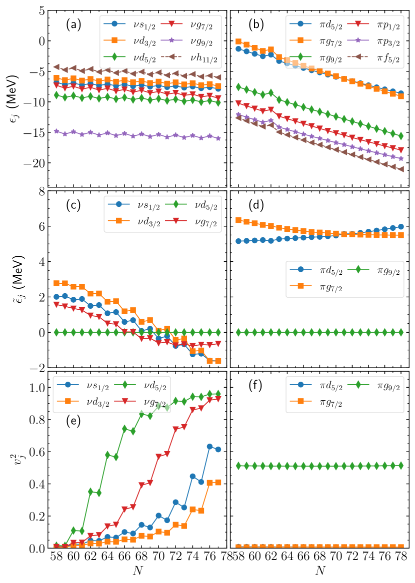
Figure 1 shows the neutron and proton spherical single-particle energies ( and ), resulting from the Gogny-HFB calculations, and the quasiparticle energies ( and ) and occupation probabilities ( and ) used in the IBFM-2 and IBFFM-2 calculations.
II.3 Electromagnetic transition operators
Theories with effective degrees of freedom, like the IBFFM, require the definition of transition operators to be used in the evaluation of electromagnetic transition probabilities. For the electric transition the operator to be used in the IBFFM-2 takes the form [31]
| (9) |
where the first and second terms are the boson and fermion parts, respectively. They are given by
| (10) |
and
| (11) |
The fixed values b for the boson effective charges are taken so that the experimental transition probabilities are reproduced for even-even Pd isotopes. The standard neutron and proton effective charges b b are employed for all the studied odd-nucleon systems. The transition operator is defined as
| (12) |
The empirical factors (nuclear magneton) and , are adopted for the neutron and proton bosons. For the neutron (proton) factors, the standard Schmidt values and ( and ) are used, with quenched by 30% with respect to the free value.
II.4 Gamow-Teller and Fermi transition operators
As in the electromagnetic case, the transition operators for allowed decay have to be redefined in terms of the relevant degrees of freedom of the model. The Gamow-Teller and Fermi transition operators take the form
| (13) | ||||
| (14) |
with the coefficients
| (15) | ||||
| (16) |
In Eqs. (13) and (14), represents one of the one-particle creation operators
| (17a) | ||||
| (17b) | ||||
| and the annihilation operators | ||||
| (17c) | ||||
| (17d) | ||||
The operators in Eqs. (17a) and (17c) conserve the boson number, whereas those in Eqs. (17b) and (17d) do not. The operators and are expressed as a combination of two of the operators in Eqs. (17a)-(17d), depending on the type of the decay studied (i.e., or ) and on the particle or hole nature of the valence nucleons. In the present case,
| (20) |
for the decay of the odd- Rh, while
| (23) |
for the decay of the even- Rh. On the other hand, for all the considered decays. Note, that Eqs. (17a)–(17d) are simplified forms of the most general one-particle transfer operators in the IBFM-2 [31].
By using the generalized seniority scheme, the coefficients , , , and in Eqs. (17a) and (17b) can be written as [68]
| (24a) | ||||
| (24b) | ||||
| (24c) | ||||
| (24d) | ||||
The factors , , and are defined as
| (25a) | ||||
| (25b) | ||||
| (25c) | ||||
where is the number operator for the boson and stands for the expectation value of a given operator in the ground state of the even-even nucleus. The amplitudes and appearing in Eqs. (24a)-(24d) and (25a)-(25c) are the same as those used in the IBFM-2 (or IBFFM-2) calculations for the odd-mass (or odd-odd) nuclei. No additional parameter is introduced for the GT and Fermi operators. For a more detailed account on -decay operators within the IBFM-2 or IBFFM-2 framework, the reader is also referred to Refs. [68, 6, 31].
The -decay values are given by
| (26) |
where the numeric constant takes the value s. The quantities and are the reduced matrix elements of the operators of Eq. (14) and of Eq. (13), respectively. Here and are the vector and axial-vector coupling constants, respectively. In this study, we use the free nucleon values, and , for the decays of both even- and odd- Rh.


III Even-even nuclei
III.1 Potential energy surfaces
The Gogny-D1M HFB and mapped IBM-2 potential energy surfaces are shown in Fig. 2 as functions of the deformation parameters for the even-even 104-124Pd nuclei. The variation of the HFB potential energy surfaces as functions of the neutron number suggests a transition from prolate (for ) to -soft (), and to nearly spherical () shapes. In particular, both 112,114Pd exhibit rather flat potential energy surfaces along the direction. This is what is expected in the -unstable O(6) limit of the IBM [29]. In the case of 116Pd, a flat-bottomed potential with a weak dependence, characteristic of the E(5) critical-point symmetry [69], is obtained.
For each of the considered nuclei, the Gogny-HFB and IBM-2 energy surfaces display a similar topology in the neighborhood of the global minimum (the location of the minimum, and the softness in the and directions are similar). However, the mapped IBM-2 surfaces generally become flat at large deformation (). This difference is a consequence of the fact that in the HFB approach all nucleonic degrees of freedom are taken into account while the IBM-2 is built on the more limited model (valence) space of nucleon pairs. However, since the mean-field configurations most relevant to the low-energy collective excitations are those in the vicinity of the global minimum, the mapping is considered specifically in that region [63, 64].


III.2 Spectroscopic properties
The mapped IBM-2 excitation energies of the , , , and states in the even-even 104-124Pd nuclei are shown in Fig. 3 as functions of the neutron number . Results obtained using the conventional IBM-2 approach (hereinafter referred to as phenomenological IBM-2), with parameters adopted from the earlier phenomenological study [37], are also included in the plot. As can be seen from the figure, the excitation energies decrease toward the middle of the major shell, i.e., . For , the mapped IBM-2 and excitation energies underestimate the experimental ones while the energies of the non-yrast and states are overestimated. In the mapped (phenomenological) IBM-2 approach the ratios of the to excitation energies are 2.96 (2.43), 2.86 (2.39), and 2.69 (2.34) for 104Pd, 106Pd, and 108Pd, respectively. These values should be compared with the experimental ratios of 2.38, 2.40, and 2.41. Thus, the mapped IBM-2 provides excitation spectra which are more rotational in character than the phenomenological IBM-2 and experimental ones. Around the neutron midshell , both the predicted and experimental levels have the lowest energies, being even below the state. The state is the bandhead of the quasi- band, and the lowering of this state reflects an emergence of pronounced softness.
The IBM-2 parameters obtained for the even-even Pd isotopes from the mapping procedure, and those determined phenomenologically are shown in Fig. 4. The phenomenological IBM-2 parameters are extracted from earlier fitting calculations for Pd and Ru isotopes [37]. In Ref. [37], in addition to the terms that appear in Eq. (2), the like-boson interactions, and the so-called Majorana terms were included in the model Hamiltonian. These terms were, however, shown to play a minor role [37], and are omitted in the present study. From Fig. 4, one sees that the single- boson energy and the strength have similar nucleon-number dependence for both the mapped and phenomenological IBM-2 models. A notable quantitative difference is that the derived values for the former are 1.4 larger in magnitude than for the latter. The behavior of the parameter is different in the two approaches for . The sign and absolute value of the sum reflect the extent of softness and whether the nucleus is prolate or oblate deformed. In both calculations, the sum is negative, , for , indicating prolate deformation, and takes nearly vanishing values, , around the neutron midshell , reflecting softness. However, for , the sum is negative (positive) in the mapped (phenomenological) calculations, implying prolate (oblate) deformation. Note that a fixed value is employed in the phenomenological IBM-2 calculations, whereas in the mapped approach this parameter exhibits a strong nucleon number dependence.
The transition probabilities, computed within the mapped and phenomenological IBM-2 models, are plotted in Fig. 5 as functions of the neutron number . The same effective boson charge is used for the quadrupole operators in the two sets of the IBM-2 calculations. The and values obtained in the mapped IBM-2 calculations agree reasonably well with the experiment, exception made of 112Pd. Both the mapped and phenomenological IBM-2 calculations predict and rates with similar trends as functions of . However, the mapped IBM-2 scheme provides smaller values for Pd isotopes with . The enhancement of the predicted transition rates around the midshell [see Fig. 5(d)] can be considered as another signature of soft deformation.


IV Odd- Pd and Rh nuclei
The excitation energies of the low-lying positive-parity states obtained for the odd- Pd isotopes 105-123Pd are depicted in Fig. 6. The results obtained within the IBFM-2 model with boson-core Hamiltonian determined by mapping the Gogny-D1M EDF [Fig. 6(a)] and the those obtained from phenomenological calculations of Ref. [37] [Fig. 6(b)] are compared with experimental data [71, 72, 70]. The two IBFM-2 calculations, using different boson-core Hamiltonian parameters, provide an overall consistent description of the experimental excitation energies. As can be seen from the figure, the experimental data display a change in the ground state spin from to 69. The corresponding even-even core nuclei, 114Pd and 116Pd, are in the transitional region, for which the potential energy surfaces are suggested to be considerably soft (see Fig. 2). The sudden change in the ground-state spin of the odd- neighbor, therefore, reflects the transition that takes place in the even-even core systems from the unstable shape, which is associated with an O(6)-like potential, to the E(5)-like structure characterized by a flat-bottomed potential.
The excitation energies of the low-lying positive-parity states obtained for the odd- isotopes 103-123Rh are depicted in Fig. 7. Experimentally, the ground states of these isotopes have spin . Exceptions are made of some of the heaviest isotopes, and similar results are predicted within both the mapped and phenomenological calculations. Both theoretically and experimentally, some of the energy levels exhibit an approximate parabolic behavior with a minimum around the middle of the major shell, . For 103-123Rh, the order of most of the energy levels remains unchanged in the whole isotopic chain within both the mapped and phenomenological IBFM-2 calculations. This situation is in a sharp contrast with the one in the odd- Pd (see Fig. 6), in which the structural change along the isotopic chain occurs more rapidly. Note that the low-lying states of the odd- Rh nuclei are accounted for almost purely by the proton single-particle configuration while more than one single-particle orbital is considered for the odd- Pd. The occupation number of the odd proton in the orbital is also nearly constant along the whole Rh isotopic chain [see Fig. 1(f)], whereas the occupation probabilities for the odd neutron in the odd- Pd vary significantly with [see Fig. 1(e)]. Furthermore, as shown below, the strength parameters for are fixed in the case of odd- Rh nuclei while they depend on the boson number for odd- Pd isotopes.
The strength parameters of the boson-fermion interaction (4) for odd- Pd nuclei are shown in Fig. 8. These parameters are chosen so that the ground-state spin, and energies of a few low-lying levels are reproduced reasonably well. The parameters for the two IBFM-2 calculations are rather similar, with an exception made of the monopole strength for . Note that common quasiparticle energies and occupation probabilities are used for both IBFM-2 calculations. The parameters for the 123Pd77 nucleus, where no experimental data are available, are taken to be the same as those for the adjacent nucleus 121Pd75. As can be seen from the figure, the IBFM-2 parameters turn out to have a strong -dependence that reflects the rapid structural change in the odd- Pd isotopes. On the other hand, constant strength parameters (0.0) MeV, (0.75) MeV, and () MeV reproduce reasonably well the experimental data for odd- Rh nuclei in the mapped (phenomenological) calculations.
| Calc. | ||||
|---|---|---|---|---|
| mapped | phen. | Expt. | ||
| 105Pd | ||||
| 107Pd | ||||
| 109Pd | ||||
| Calc. | ||||
|---|---|---|---|---|
| mapped | phen. | Expt. | ||
| 103Rh | ||||
| 107Rh | ||||
| 109Rh | ||||
Experimental data for electromagnetic transitions and moments are available for odd- Pd and Rh nuclei with . The predicted and transition strengths as well as the electric quadrupole and magnetic dipole moments for the low-lying positive-parity states in odd- Pd are given in Table 2. In most of the cases, the mapped and phenomenological calculations provide similar results. Large values are obtained for the (in 105Pd, 107Pd and 109Pd), (in 105Pd and 109Pd), and (in 105Pd) transitions. The experimental data, however, suggest that these transitions are weaker. The and rates corresponding to some transitions in odd- Rh nuclei are given in Table 3. The large and rates obtained for 103Rh overestimate the experimental rates by several orders of magnitude.
The deviation of the predicted and transition rates for odd- systems with respect to the experiment could be interpreted in terms of the structure of the corresponding IBFM-2 wave functions. The components of the IBFM-2 wave functions for the low-lying states of odd- Pd isotopes are shown in Fig. 9. They are associated with the single(quasi)-particle orbitals , , , and . Only components obtained within the mapped framework are shown as illustrative examples, while qualitatively similar results are obtained using the phenomenological approach. The states considered for odd- Rh nuclei are almost purely made of the proton configuration (with a weight of %). Therefore, the corresponding wave function contents are not shown in the plot. As can be seen from the figure, the neutron configuration accounts for most of the IBFM-2 wave functions for the , , , and in odd- Pd nuclei with . However, the description of these wave functions in both the mapped and phenomenological IBFM-2 calculations in the present study may not be adequate, and this leads to some of the considerable disagreements between the calculated and experimental electromagnetic properties, including the values in 105Pd, 107Pd, and 109Pd (see Table 2). The deficiency of the IBFM-2 wave functions could arise from various deficiencies of the present model calculations, such as the choice of the single-particle space, the quasiparticle energies and occupation probabilities of the odd particle, and the effective charges involved in the transition operators, which are kept constant for all nuclei. On the other hand, earlier IBFM-2 fitting calculations in the same mass region [74, 7] obtained and properties consistent with experiment.


V Odd-odd Rh nuclei
The excitation energies of the low-lying positive-parity states obtained for odd-odd Rh isotopes are depicted in Fig. 10. The available experimental data [70] suggest that for the ground state has spin . Excited states are also observed at low energy. Both the mapped [Fig. 10(a)] and phenomenological [Fig. 10(b)] IBFFM-2 calculations account for the ground-state spin . The calculations also reproduce reasonably well the energies of the states. From to 73, both types of calculations suggest a change in the ground-state spin to . There are no spectroscopic data to compare with for even- Rh isotopes with . Note, that a ground-state spin different from is experimentally found in the neighboring odd-odd Ag and In isotopes. For instance, for 120Ag, 122Ag, 124Ag and 126In the ground state has spin . A low-lying level is observed in 122In at an excitation energy around 40 keV above the ground state.
The strength parameters and of the neutron-proton residual interaction in Eq. (II.1) are shown in Fig. 11 for odd-odd Rh isotopes as functions of the neutron number. Those parameters are determined so that the correct ground-state spin as well as the energy of the state are reproduced reasonably well. For , where experimental data are not available, the same values of the parameters as for 116Rh71 are employed. As can be seen from Fig. 11(a), the parameter changes suddenly from to 67. This sudden change accounts for the experimental [see Fig. 10(c)] lowering of the level toward the middle of the major shell, . On the other hand, the tensor interaction strength exhibits a smooth decrease with .

The nature of the low-lying states in odd-odd Rh isotopes can be analyzed in terms of various neutron-proton pair components in the IBFFM-2 wave functions. The corresponding results for the and states, obtained within the mapped IBFFM-2 formalism, are shown in Fig. 12. For nuclei with , the state is mostly based on the configuration associated with the neutron-proton pairs coupled to the even-even boson core, with the total angular momentum of the fermion system , 8. For 120Rh and 122Rh, the contributions of the () pairs also play a prominent role. As one can see from Fig. 12(b), the dominant contribution to the wave function for Rh isotopes with mass comes from the pair components, while the pair components play a negligible role. For heavier Rh isotopes, with , the other pair components that involve the state, i.e., those based on the , , and pairs, are rather fragmented in the wave functions. Qualitatively similar results are obtained using phenomenological IBFFM-2 wave functions.
| Calc. | ||||
|---|---|---|---|---|
| mapped | phen. | Expt. | ||
| 104Rh | ||||
| 106Rh | ||||
The experimental information on the electromagnetic properties of the considered odd-odd Rh nuclei is rather limited. Table 4 compares the predicted and experimental , , and magnetic dipole moment for 104Rh and 106Rh. Both the mapped and phenomenological IBFFM-2 calculations provide a reasonable description of the experimental data for these odd-odd nuclei. Nevertheless, a more detailed assessment of the quality of the IBFFM-2 wave functions is difficult in this case, due to the lack of data.
| Calc. | ||||
|---|---|---|---|---|
| Decay | mapped | phen. | Expt. | |
| 105RhPd | 7.45 | 6.88 | 5.710(7) | |
| 8.12 | 7.66 | 5.797(16) | ||
| 7.19 | 7.41 | 5.152(20) | ||
| 9.01 | 10.08 | 6.91(3) | ||
| 107RhPd | 6.81 | 6.47 | 6.1(2) | |
| 7.81 | 7.39 | 5.0(1) | ||
| 7.78 | 6.99 | 6.2(1) | ||
| 6.23 | 8.05 | 5.8(1) | ||
| 8.00 | 7.45 | 6.1(1) | ||
| 5.82 | 7.87 | 5.3(1) | ||
| 109RhPd | 6.05 | 5.86 | 5.8(3) | |
| 7.02 | 6.19 | 6.69(12) | ||
| 6.92 | 6.58 | 4.86(5) | ||
| 5.68 | 5.57 | 5.69(6) | ||
| 6.83 | 7.39 | 5.53(5) | ||
| 7.32 | 6.84 | 7.26(19) | ||
| 113RhPd | 4.58 | 4.51 | 5.4(1) | |
| 6.46 | 8.07 | 5.90(5) | ||
| 4.35 | 4.28 | 5.00(4)111 at 349 keV [70] | ||
| 5.71 | 5.57 | 5.00(4)111 at 349 keV [70] | ||
| 5.42 | 5.59 | 6.7(2)222 at 373 keV based on the XUNDL datasets [70] | ||
| 5.07 | 4.81 | 6.7(2)222 at 373 keV based on the XUNDL datasets [70] | ||
| 117RhPd | 5.61 | 5.09 | 6.0333Uncertainties are not given with the . | |
| 5.81 | 5.31 | 5.7333Uncertainties are not given with the . | ||
| 4.27 | 5.34 | 5.8333Uncertainties are not given with the . | ||
| 5.22 | 5.27 | 6.3333Uncertainties are not given with the . | ||
| 7.64 | 4.56 | 6.3333Uncertainties are not given with the . | ||
| 5.82 | 5.50 | 6.0444 level at 436 keV, based on the XUNDL datasets [70]. Uncertainties are not given. | ||
| 4.97 | 5.28 | 6.0444 level at 436 keV, based on the XUNDL datasets [70]. Uncertainties are not given. | ||
VI decay
VI.1 decays between odd- nuclei
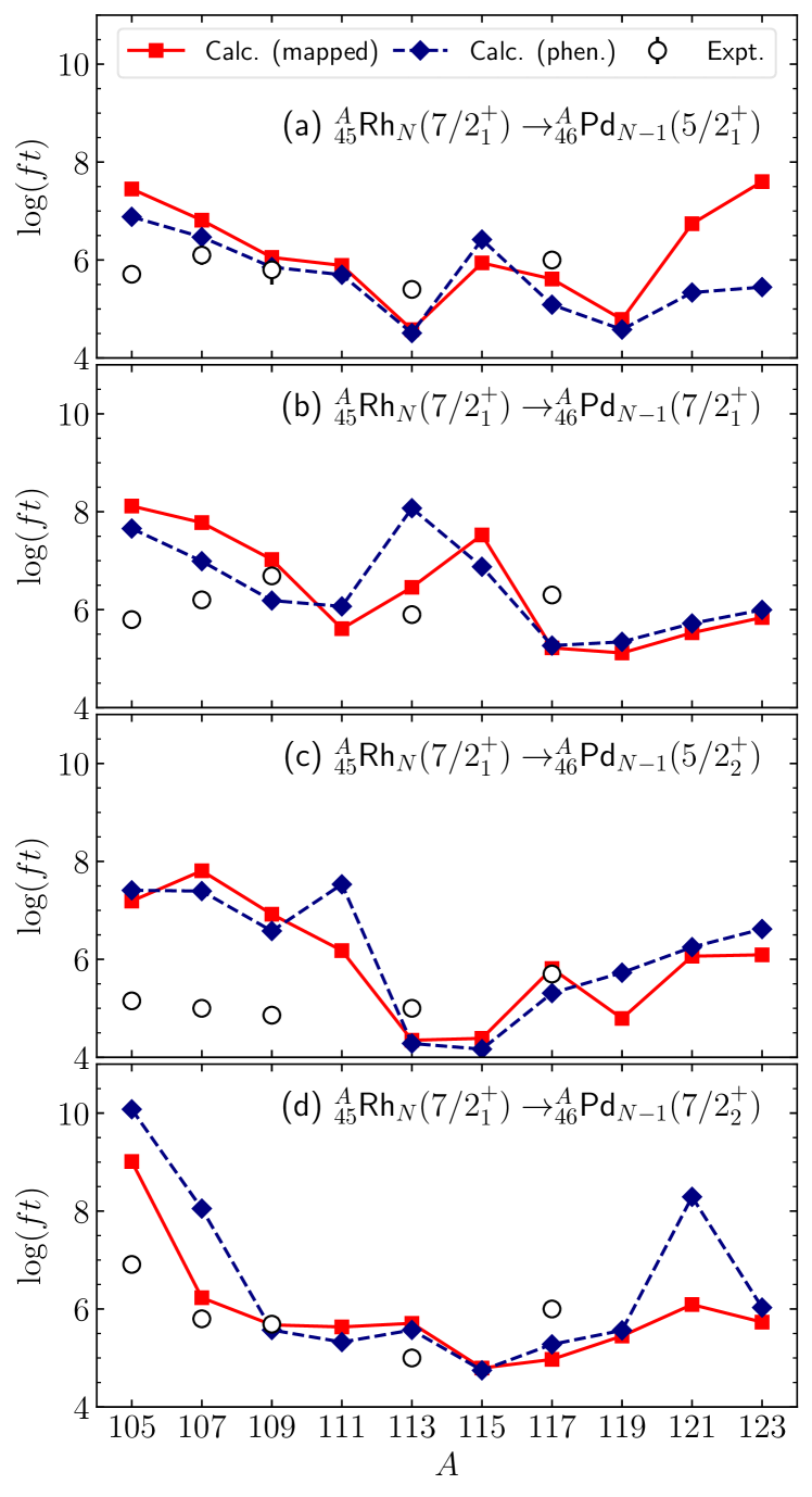
Figure 13 shows the values for the decays of the state of the odd- Rh into several low-lying states of the odd- Pd nuclei. Results are obtained using mapped and phenomenological IBFM-2 wave functions. In both cases, the predicted trend of the values, as functions of the nucleon number, reflects the structural change in the parent and daughter odd- nuclei. An illustrative example is a kink emerging at the mass or 115 in the predicted values for the [Fig. 13(a)] and [Fig. 13(b)] decays. The mass number at which the kink emerges corresponds to the transitional region, where the ground-state spin changes, observed in the odd- Pd daughter (see Fig. 6). The mass dependence of the predicted values is similar in the mapped and phenomenological calculations, exception made of the results from =113 to 115 in the decay and from =117 to 119 in the decay.
Both within the mapped and phenomenological schemes, the present calculations overestimate the observed values for the decays 105,107RhPd [Fig. 13(a)]. At both 105 and 107, the final-state wave function has been shown to be almost purely made of the configuration [see Fig. 9(c)], while the parent state is of almost pure nature.
The dominant contribution to the GT matrix element for the above decays indeed comes from the term that corresponds to the coupling of the with single-particle states, which is of the form
| (27) |
The matrix element of this term is, however, rather small: 0.041 and (0.069 and ), for the 105Rh and 107Rh decays in the mapped (phenomenological) approach. There are many other terms similar to the one in Eq. (27), but their matrix elements are small and cancel each other, leading to a small GT transition rate. The same is true for the 105,107RhPd decays [Fig. 13(b)]. In this case, the Fermi transition matrix is also negligibly small.
The calculations underestimate the values for the 113RhPd decay. For this decay, approximately 75 % and 25 % of the wave function of the final state are comprised of the and configurations, respectively [see Fig. 9(c)]. Due to the large admixture of the components into the state of 113Pd, the term that is proportional to
| (28) |
makes a sizable contribution to the GT transition strength. The matrix element of this component, which amounts to (0.850) in the mapped (phenomenological) calculation, is so large that the corresponding value is too small as compared with the experimental value.
As noted above, there are notable quantitative differences between the mapped and phenomenological predictions for the values in the case of the 113RhPd decay. The GT transition matrix element obtained in the phenomenological calculation is two orders of magnitude smaller than the one obtained within the mapped scheme. This difference stems from a subtle balance between matrix elements of different terms in the GT transition operator. The dominant contribution to the GT matrix element in the former calculation come from the term proportional to the expression in Eq. (28), and the one of the form
| (29) |
Their matrix elements are of the same order of magnitude, but have the opposite signs, hence cancellation occurs between these terms. The degree of the cancellation, however, is much smaller in the mapped calculation. The contribution of the Fermi matrix element is negligibly small in both the mapped and phenomenological cases.
The values for the Rh decays into the non-yrast states, and , of the odd- Pd are shown in Figs. 13(c) and 13(d), respectively. The predicted values for the ARhPd decay in the two sets of calculations are generally large, for . In particular, they overestimate the experimental values for the 105Rh, 107Rh, and 109Rh decays by a factor of two. The discrepancy could be attributed to the nature of the IBFM-2 wave functions and the components of the GT operator. The computed values for the ARhPd decay in the mapped scheme are close to the experimental values, with an exception made of the 105Rh decay.
Table 5 gives complementary results for the values of the decays ARhPd, with final states other than those already discussed above. The predicted values are compared with the available experimental data [70].
Previous IBFM-2 calculations [7] provided values for the decays and in 105,107,109Rh which are consistent with the experimental ones. However, for the same nuclei the values 4 were obtained for the decay. Such values are systematically smaller than the experimental values and those obtained in this work. A more recent IBFM-2 calculation for the 115,117RhPd decay [13] obtained a value = 5.90 for the decay of 115Rh. This value is close to the one obtained in this study. On the other hand, for the and decays of 117Rh, the values = 6.78 and 6.68 were reported in [13]. They are approximately 20 % larger than those obtained in the present work.


VI.2 decays of even- nuclei
The values for the decays of the even- Rh into Pd nuclei are plotted in Fig. 14. One immediately sees from Fig. 14(a) that the mapped and phenomenological values for the ARhPd decays are, approximately, a factor two smaller than the experimental ones. The corresponding GT matrix elements are almost purely determined by the contributions of the terms associated with the coupling, i.e.,
| (30) |
for and
| (31) |
for . As shown in Fig. 15(a), the matrix elements of these terms are particularly large for the mass . Note also, that the IBFFM-2 wave functions for the initial state mainly consist of the pair configuration for the even- Rh with [see Fig. 12(a)]. For the larger mass , this pair configuration becomes less important in the wave function of the final nucleus. As a consequence, the GT transition strength decreases with increasing [see Fig. 15(a)].
To reproduce the -decay data, effective values of the factor, , are often employed. Here we compare the predicted value for the ARhPd decay with the corresponding experimental one, and extract the values for those decays for which data are available. The resulting values are, on average, (0.205) in the mapped (phenomenological) scheme. This amounts to a reduction of the free value by approximately by 88 (84) %. In the previous IBM-2/IBFFM-2 study of the and decays of the Te and Xe isotopes with [9], the values extracted from a comparison with the data for the single- decays are 0.313 for the decay 128ITe, and 0.255 for the decay 128IXe.
As can be seen from Fig. 14(b), the values obtained within the mapped and phenomenological approaches for the ARhPd decay differ considerably. The difference between the two calculations is especially large at and 116. One sees from Fig. 15(b), that the GT matrix element for the 116Rh decay in the phenomenological calculations is much larger in magnitude than the one obtained within the mapped approach, with the largest contribution coming from the term associated with the coupling. Generally, the predicted values for the decay, both within the mapped and phenomenological schemes, increase with (or ). This is due to the fact that the pair configuration gradually becomes less important in the wave function of the even- Rh for larger [see Fig. 12(a)].
For the ARhPd decay, the values predicted within the mapped and phenomenological approaches are similar. The most notable difference occurs at , with the mapped value being nearly half the phenomenological one. This is a consequence of the fact that in the mapped GT matrix element associated with the 116Rh decay, the component of Eq. (31) is an order of magnitude larger than the one in the phenomenological calculations [see Fig. 15(c)]. In addition, the computed values for the decay are larger than those for the decay because the matrix elements of the components involving the coupling in the strength are smaller in magnitude than those in the one.
The values corresponding to the ARhPd decay are depicted in Fig. 14(d). Both the mapped and phenomenological calculations largely underestimate the measured value at . However, the results obtained with both schemes reproduce the experimental trend reasonably well for . As can be seen from Fig. 15(d), the difference between the mapped and phenomenological results for is due to the difference between the matrix elements for the components in both schemes, with the mapped matrix elements being an order of magnitude smaller than the phenomenological ones.
| Calc. | ||||
|---|---|---|---|---|
| Decay | mapped | phen. | Expt. | |
| 104RhPd | 3.27 | 3.21 | 4.55(1) | |
| 3.54 | 5.41 | 5.80(1) | ||
| 5.91 | 5.85 | 7.36(2) | ||
| 6.03 | 4.45 | 8.7(1) | ||
| 6.42 | 6.05 | 5.5(1) | ||
| 5.24 | 4.72 | 6.3(1) | ||
| 7.26 | 8.30 | 7.3(1) | ||
| 8.45 | 7.59 | 6.1(1) | ||
| 8.06 | 8.04 | 6.2(1) | ||
| 8.59 | 8.57 | 5.8(1) | ||
| 106RhPd | 3.31 | 3.43 | 5.168(7) | |
| 3.72 | 4.29 | 5.865(17) | ||
| 6.78 | 4.72 | 6.55(7) | ||
| 5.39 | 6.82 | 5.354(19) | ||
| 5.15 | 4.58 | 5.757(17) | ||
| 108RhPd | 3.31 | 3.45 | 5.5(3) | |
| 3.97 | 4.14 | 5.7(4) | ||
| 7.06 | 5.00 | 6.0(4) | ||
| 5.07 | 6.01 | 5.6(4) | ||
| 7.72 | 7.44 | 6.8(3) | ||
| 8.28 | 7.00 | 4.84(9)111 level at 2864 keV | ||
| 9.59 | 8.35 | 4.84(9)111 level at 2864 keV | ||
| 9.30 | 9.42 | 4.84(9)111 level at 2864 keV | ||
| 110RhPd | 8.29 | 8.26 | 6.38(13) | |
| 9.57 | 8.95 | 7.1(4) | ||
| 9.16 | 8.69 | 6.34(25) | ||
| 112RhPd | 3.55 | 3.61 | 5.5 | |
| 4.88 | 4.35 | 6.2(3) | ||
| 5.53 | 5.86 | 6.4(3) | ||
| 6.20 | 5.01 | 6.52(6) | ||
| 7.48 | 6.36 | 6.88(9)222 level at 1140 keV | ||
| 7.74 | 5.66 | 6.88(9)222 level at 1140 keV | ||
| 5.83 | 5.39 | 6.88(9)222 level at 1140 keV | ||
| 5.83 | 5.39 | 6.97(22) | ||
| 5.83 | 5.39 | 6.50(7) | ||
| 8.75 | 8.80 | 6.52333 values should be considered approximate [70]. | ||
| 8.96 | 10.34 | 6.54 | ||
| 9.15 | 8.82 | 6.88 | ||
| 114RhPd | 3.59 | 4.37 | 5.9(2) | |
| 5.19 | 3.89 | 6.0(4) | ||
| 6.60 | 6.08 | 5.7(2) | ||
| 4.59 | 5.10 | 6.1(2) | ||
| 5.57 | 5.28 | 6.1(2) | ||
| 116RhPd | 3.75 | 4.38 | 5.62(22) | |
| 6.36 | 4.04 | 5.84(18) | ||
| 6.99 | 6.63 | 5.76(19) | ||
| 4.45 | 8.03 | 6.47(20) | ||
| 5.29 | 8.60 | 6.36(19) | ||
| 5.05 | 5.00 | 6.81(21) | ||
For the sake of completeness, Table 6 compares the predicted and experimental [70] values for the decays of the even- Rh isotopes. Cases other than hose already discussed above are considered in the table. As compared with the ground-state-to-ground-state decay , the values for the decays of the state into non-yrast and states, and the values for the and decays are calculated to be large. Note that the predicted values for the decays 104RhPd and 108RhPd are rather close to the experimental ones.
VII Conclusions
In this paper, the low-energy collective states and decays for even and odd-mass neutron-rich Rh and Pd isotopes have been studied using a mapping framework based on the Gogny-EDF and the particle-boson coupling scheme. The constrained HFB has been employed to provide microscopic input to the mapping procedure. Such an input consists of potential energy surfaces as functions of the shape degrees of freedom for the even-even 104-124Pd isotopes. The IBM-2 Hamiltonian, used to describe even-even core nuclei, has been determined by mapping the Gogny-D1M HFB fermionic potential energy surfaces onto the corresponding bosonic surfaces. The microscopic mean-field calculations also provided single-particle energies for the odd systems. Those represent essential building blocks of the boson-fermion interactions for the neighboring odd- and odd-odd nuclei as well as for the GT and Fermi transition operators. The strength parameters of the boson-fermion and residual neutron-proton interactions were fitted to low-energy data for the odd- and odd-odd systems.
The Gogny-HFB potential energy surfaces obtained for even-even Pd isotopes point towards a transition from prolate deformed (104-108Pd) to -soft (110-116Pd), and to nearly spherical shapes (118-124Pd). The low-energy excitation spectra and transition strengths resulting from the diagonalization of the mapped IBM-2 Hamiltonian reproduced the experimental trends reasonably well and reflect, to a large extent, the structural evolution of the ground-state shapes predicted at the mean-field level. The excitation energies obtained for the low-lying positive-parity levels in the odd- Pd and Rh, and even- Rh nuclei also exhibit signatures of this structural evolution. Within this context, a notable example is the change in the ground state spin from 113Pd to 115Pd. The computed values for the decays of the odd- and even- Rh into Pd nuclei have been shown to be sensitive to the nature of the wave functions of the parent and daughter nuclei. They also reflect the rapid structural evolution along the considered isotopic chains. The values for the odd- Rh decay have been predicted to be larger than the experimental ones for . This could be traced back to the structure of the IBFM-2 wave functions for the odd- daughter (Pd) nuclei. Furthermore, it has been shown that for the even- Rh decay, the neutron-proton pair components play a key role in the GT transition matrix elements and are responsible for the too small values for the ARhPd decay with respect to the experimental data.
The results of the mapped calculations have been compared with conventional IBM-2 calculations in which the parameters for the boson Hamiltonian have been fit to the experiment. The mapped and phenomenological IBM-2 excitation spectra for even-even, odd-, and odd-odd systems are similar. However, the two sets of calculations differ in their predictions for electromagnetic and -decay properties of the odd-nucleon systems.
The results obtained in this study could be considered a plausible step towards a consistent simultaneous description of the low-lying states and -decay properties of atomic nuclei. However, the difference between the predicted and experimental -decay values might require additional refinements of the employed theoretical framework. In particular, the small values obtained suggest that the role of the effective axial-vector coupling constant should be further studied in future calculations. The values extracted in this work from the comparison with the experimental data turned out to be by a factor 7-8 smaller than the free nucleon value. This large quenching indicates deficiencies in the model space of the calculations or of the theoretical procedure itself. Investigation along these lines is in progress and will be reported elsewhere.
Acknowledgements.
This work is financed within the Tenure Track Pilot Programme of the Croatian Science Foundation and the École Polytechnique Fédérale de Lausanne, and Project No. TTP-2018-07-3554 Exotic Nuclear Structure and Dynamics, with funds of the Croatian-Swiss Research Programme. The work of LMR is supported by the Spanish Ministry of Economy and Competitiveness (MINECO) Grant No. PGC2018-094583-B-I00.References
- Nishimura et al. [2011] S. Nishimura, Z. Li, H. Watanabe, K. Yoshinaga, T. Sumikama, T. Tachibana, K. Yamaguchi, M. Kurata-Nishimura, G. Lorusso, Y. Miyashita, A. Odahara, H. Baba, J. S. Berryman, N. Blasi, A. Bracco, F. Camera, J. Chiba, P. Doornenbal, S. Go, T. Hashimoto, S. Hayakawa, C. Hinke, E. Ideguchi, T. Isobe, Y. Ito, D. G. Jenkins, Y. Kawada, N. Kobayashi, Y. Kondo, R. Krücken, S. Kubono, T. Nakano, H. J. Ong, S. Ota, Z. Podolyák, H. Sakurai, H. Scheit, K. Steiger, D. Steppenbeck, K. Sugimoto, S. Takano, A. Takashima, K. Tajiri, T. Teranishi, Y. Wakabayashi, P. M. Walker, O. Wieland, and H. Yamaguchi, Phys. Rev. Lett. 106, 052502 (2011).
- Lorusso et al. [2015] G. Lorusso, S. Nishimura, Z. Y. Xu, A. Jungclaus, Y. Shimizu, G. S. Simpson, P.-A. Söderström, H. Watanabe, F. Browne, P. Doornenbal, G. Gey, H. S. Jung, B. Meyer, T. Sumikama, J. Taprogge, Z. Vajta, J. Wu, H. Baba, G. Benzoni, K. Y. Chae, F. C. L. Crespi, N. Fukuda, R. Gernhäuser, N. Inabe, T. Isobe, T. Kajino, D. Kameda, G. D. Kim, Y.-K. Kim, I. Kojouharov, F. G. Kondev, T. Kubo, N. Kurz, Y. K. Kwon, G. J. Lane, Z. Li, A. Montaner-Pizá, K. Moschner, F. Naqvi, M. Niikura, H. Nishibata, A. Odahara, R. Orlandi, Z. Patel, Z. Podolyák, H. Sakurai, H. Schaffner, P. Schury, S. Shibagaki, K. Steiger, H. Suzuki, H. Takeda, A. Wendt, A. Yagi, and K. Yoshinaga, Phys. Rev. Lett. 114, 192501 (2015).
- Quinn et al. [2012] M. Quinn, A. Aprahamian, J. Pereira, R. Surman, O. Arndt, T. Baumann, A. Becerril, T. Elliot, A. Estrade, D. Galaviz, T. Ginter, M. Hausmann, S. Hennrich, R. Kessler, K.-L. Kratz, G. Lorusso, P. F. Mantica, M. Matos, F. Montes, B. Pfeiffer, M. Portillo, H. Schatz, F. Schertz, L. Schnorrenberger, E. Smith, A. Stolz, W. B. Walters, and A. Wöhr, Phys. Rev. C 85, 035807 (2012).
- Avignone et al. [2008] F. T. Avignone, S. R. Elliott, and J. Engel, Rev. Mod. Phys. 80, 481 (2008).
- Navrátil and Dobe [1988] P. Navrátil and J. Dobe, Phys. Rev. C 37, 2126 (1988).
- Dellagiacoma and Iachello [1989] F. Dellagiacoma and F. Iachello, Phys. Lett. B 218, 399 (1989).
- Yoshida et al. [2002] N. Yoshida, L. Zuffi, and S. Brant, Phys. Rev. C 66, 014306 (2002).
- Brant et al. [2004] S. Brant, N. Yoshida, and L. Zuffi, Phys. Rev. C 70, 054301 (2004).
- Yoshida and Iachello [2013] N. Yoshida and F. Iachello, Prog. Theor. Exp. Phys. 2013, 043D01 (2013).
- Mardones et al. [2016] E. Mardones, J. Barea, C. E. Alonso, and J. M. Arias, Phys. Rev. C 93, 034332 (2016).
- Nomura et al. [2020a] K. Nomura, R. Rodríguez-Guzmán, and L. M. Robledo, Phys. Rev. C 101, 024311 (2020a).
- Nomura et al. [2020b] K. Nomura, R. Rodríguez-Guzmán, and L. M. Robledo, Phys. Rev. C 101, 044318 (2020b).
- Ferretti et al. [2020] J. Ferretti, J. Kotila, R. I. M. n. Vsevolodovna, and E. Santopinto, Phys. Rev. C 102, 054329 (2020).
- Nomura [2022] K. Nomura, Phys. Rev. C 105, 044306 (2022).
- Álvarez-Rodríguez et al. [2004] R. Álvarez-Rodríguez, P. Sarriguren, E. M. de Guerra, L. Pacearescu, A. Faessler, and F. Šimkovic, Phys. Rev. C 70, 064309 (2004).
- Sarriguren [2015] P. Sarriguren, Phys. Rev. C 91, 044304 (2015).
- Boillos and Sarriguren [2015] J. M. Boillos and P. Sarriguren, Phys. Rev. C 91, 034311 (2015).
- Pirinen and Suhonen [2015] P. Pirinen and J. Suhonen, Phys. Rev. C 91, 054309 (2015).
- Šimkovic et al. [2013] F. Šimkovic, V. Rodin, A. Faessler, and P. Vogel, Phys. Rev. C 87, 045501 (2013).
- Mustonen and Engel [2016] M. T. Mustonen and J. Engel, Phys. Rev. C 93, 014304 (2016).
- Suhonen [2017] J. T. Suhonen, Frontiers Phys. 5, 55 (2017).
- Ravlić et al. [2021] A. Ravlić, E. Yüksel, Y. F. Niu, and N. Paar, Phys. Rev. C 104, 054318 (2021).
- Minato et al. [2021] F. Minato, T. Marketin, and N. Paar, Phys. Rev. C 104, 044321 (2021).
- Langanke and Martínez-Pinedo [2003] K. Langanke and G. Martínez-Pinedo, Rev. Mod. Phys. 75, 819 (2003).
- Caurier et al. [2005] E. Caurier, G. Martínez-Pinedo, F. Nowacki, A. Poves, and A. P. Zuker, Rev. Mod. Phys. 77, 427 (2005).
- Yoshida et al. [2018] S. Yoshida, Y. Utsuno, N. Shimizu, and T. Otsuka, Phys. Rev. C 97, 054321 (2018).
- Suzuki et al. [2018] T. Suzuki, S. Shibagaki, T. Yoshida, T. Kajino, and T. Otsuka, Astrophys. J. 859, 133 (2018).
- Kumar et al. [2020] A. Kumar, P. C. Srivastava, J. Kostensalo, and J. Suhonen, Phys. Rev. C 101, 064304 (2020).
- Iachello and Arima [1987] F. Iachello and A. Arima, The interacting boson model (Cambridge University Press, Cambridge, 1987).
- Iachello and Scholten [1979] F. Iachello and O. Scholten, Phys. Rev. Lett. 43, 679 (1979).
- Iachello and Van Isacker [1991] F. Iachello and P. Van Isacker, The interacting boson-fermion model (Cambridge University Press, Cambridge, 1991).
- Brant et al. [1984] S. Brant, V. Paar, and D. Vretenar, Z. Phys. A 319, 355 (1984).
- Ring and Schuck [1980] P. Ring and P. Schuck, The nuclear many-body problem (Springer, Berlin, 1980).
- Goriely et al. [2009] S. Goriely, S. Hilaire, M. Girod, and S. Péru, Phys. Rev. Lett. 102, 242501 (2009).
- J. Decharge and M. Girod and D. Gogny [1975] J. Decharge and M. Girod and D. Gogny, Phys. Lett. B 55, 361 (1975).
- Robledo et al. [2019] L. M. Robledo, T. R. Rodríguez, and R. R. Rodríguez-Guzmán, J. Phys. G: Nucl. Part. Phys. 46, 013001 (2019).
- Van Isacker and Puddu [1980] P. Van Isacker and G. Puddu, Nucl. Phys. A 348, 125 (1980).
- Bender et al. [2003] M. Bender, P.-H. Heenen, and P.-G. Reinhard, Rev. Mod. Phys. 75, 121 (2003).
- Vretenar et al. [2005] D. Vretenar, A. V. Afanasjev, G. A. Lalazissis, and P. Ring, Phys. Rep. 409, 101 (2005).
- Nikšić et al. [2011] T. Nikšić, D. Vretenar, and P. Ring, Prog. Part. Nucl. Phys. 66, 519 (2011).
- Berger et al. [1984] J. F. Berger, M. Girod, and D. Gogny, Nucl. Phys. A 428, 23 (1984).
- Borrajo and Egido [2016] M. Borrajo and J. L. Egido, The European Physical Journal A 52, 277 (2016).
- Garrett et al. [2020] P. E. Garrett, T. R. Rodríguez, A. Diaz Varela, K. L. Green, J. Bangay, A. Finlay, R. A. E. Austin, G. C. Ball, D. S. Bandyopadhyay, V. Bildstein, S. Colosimo, D. S. Cross, G. A. Demand, P. Finlay, A. B. Garnsworthy, G. F. Grinyer, G. Hackman, B. Jigmeddorj, J. Jolie, W. D. Kulp, K. G. Leach, A. C. Morton, J. N. Orce, C. J. Pearson, A. A. Phillips, A. J. Radich, E. T. Rand, M. A. Schumaker, C. E. Svensson, C. Sumithrarachchi, S. Triambak, N. Warr, J. Wong, J. L. Wood, and S. W. Yates, Phys. Rev. C 101, 044302 (2020).
- Siciliano et al. [2020] M. Siciliano, I. Zanon, A. Goasduff, P. R. John, T. R. Rodríguez, S. Péru, I. Deloncle, J. Libert, M. Zielińska, D. Ashad, D. Bazzacco, G. Benzoni, B. Birkenbach, A. Boso, T. Braunroth, M. Cicerchia, N. Cieplicka-Oryńczak, G. Colucci, F. Davide, G. de Angelis, B. de Canditiis, A. Gadea, L. P. Gaffney, F. Galtarossa, A. Gozzelino, K. Hadyńska-Klȩk, G. Jaworski, P. Koseoglou, S. M. Lenzi, B. Melon, R. Menegazzo, D. Mengoni, A. Nannini, D. R. Napoli, J. Pakarinen, D. Quero, P. Rath, F. Recchia, M. Rocchini, D. Testov, J. J. Valiente-Dobón, A. Vogt, J. Wiederhold, and W. Witt, Phys. Rev. C 102, 014318 (2020).
- Siciliano et al. [2021] M. Siciliano, J. J. Valiente-Dobón, A. Goasduff, T. R. Rodríguez, D. Bazzacco, G. Benzoni, T. Braunroth, N. Cieplicka-Oryńczak, E. Clément, F. C. L. Crespi, G. de France, M. Doncel, S. Ertürk, C. Fransen, A. Gadea, G. Georgiev, A. Goldkuhle, U. Jakobsson, G. Jaworski, P. R. John, I. Kuti, A. Lemasson, H. Li, A. Lopez-Martens, T. Marchi, D. Mengoni, C. Michelagnoli, T. Mijatović, C. Müller-Gatermann, D. R. Napoli, J. Nyberg, M. Palacz, R. M. Pérez-Vidal, B. Sayği, D. Sohler, S. Szilner, and D. Testov, Phys. Rev. C 104, 034320 (2021).
- Rodríguez-Guzmán et al. [2020] R. Rodríguez-Guzmán, Y. M. Humadi, and L. M. Robledo, J. Phys. G: Nucl. Part. Phys. 48, 015103 (2020).
- Rodríguez-Guzmán and Robledo [2021] R. Rodríguez-Guzmán and L. M. Robledo, Phys. Rev. C 103, 044301 (2021).
- Rodríguez-Guzmán et al. [2021] R. Rodríguez-Guzmán, L. M. Robledo, K. Nomura, and N. C. Hernandez, J. Phys. G: Nucl. Part. Phys. 49, 015101 (2021).
- Nomura et al. [2012] K. Nomura, R. Rodríguez-Guzmán, L. M. Robledo, and N. Shimizu, Phys. Rev. C 86, 034322 (2012).
- Nomura et al. [2013] K. Nomura, R. Rodríguez-Guzmán, and L. M. Robledo, Phys. Rev. C 87, 064313 (2013).
- Nomura et al. [2016a] K. Nomura, R. Rodríguez-Guzmán, and L. M. Robledo, Phys. Rev. C 94, 044314 (2016a).
- Nomura et al. [2015] K. Nomura, R. Rodríguez-Guzmán, and L. M. Robledo, Phys. Rev. C 92, 014312 (2015).
- Nomura et al. [2020c] K. Nomura, R. Rodríguez-Guzmán, Y. M. Humadi, L. M. Robledo, and J. E. García-Ramos, Phys. Rev. C 102, 064326 (2020c).
- Nomura et al. [2021a] K. Nomura, R. Rodríguez-Guzmán, L. Robledo, and J. García-Ramos, Phys. Rev. C 103, 044311 (2021a).
- Nomura et al. [2021b] K. Nomura, R. Rodríguez-Guzmán, L. M. Robledo, J. E. García-Ramos, and N. C. Hernández, Phys. Rev. C 104, 044324 (2021b).
- Nomura et al. [2021c] K. Nomura, R. Rodríguez-Guzmán, and L. M. Robledo, Phys. Rev. C 104, 054320 (2021c).
- Otsuka et al. [1978a] T. Otsuka, A. Arima, and F. Iachello, Nucl. Phys. A 309, 1 (1978a).
- Otsuka et al. [1978b] T. Otsuka, A. Arima, F. Iachello, and I. Talmi, Phys. Lett. B 76, 139 (1978b).
- Scholten [1985] O. Scholten, Prog. Part. Nucl. Phys. 14, 189 (1985).
- Brant and Paar [1988] S. Brant and V. Paar, Z. Phys. A 329, 151 (1988).
- Bohr and Mottelson [1975] A. Bohr and B. R. Mottelson, Nuclear Structure (Benjamin, New York, 1975).
- Ginocchio and Kirson [1980] J. N. Ginocchio and M. W. Kirson, Nucl. Phys. A 350, 31 (1980).
- Nomura et al. [2008] K. Nomura, N. Shimizu, and T. Otsuka, Phys. Rev. Lett. 101, 142501 (2008).
- Nomura et al. [2010] K. Nomura, N. Shimizu, and T. Otsuka, Phys. Rev. C 81, 044307 (2010).
- Nomura et al. [2016b] K. Nomura, T. Nikšić, and D. Vretenar, Phys. Rev. C 93, 054305 (2016b).
- Nomura et al. [2017] K. Nomura, R. Rodríguez-Guzmán, and L. M. Robledo, Phys. Rev. C 96, 064316 (2017).
- Nomura et al. [2019] K. Nomura, R. Rodríguez-Guzmán, and L. M. Robledo, Phys. Rev. C 99, 034308 (2019).
- Dellagiacoma [1988] F. Dellagiacoma, Beta decay of odd mass nuclei in the interacting boson-fermion model, Ph.D. thesis, Yale University (1988).
- Iachello [2000] F. Iachello, Phys. Rev. Lett. 85, 3580 (2000).
- [70] Brookhaven National Nuclear Data Center, http://www.nndc.bnl.gov.
- Kurpeta et al. [2018] J. Kurpeta et al., Phys. Rev. C 98, 024318 (2018).
- Kurpeta et al. [2022] J. Kurpeta et al., Phys. Rev. C 105, 034316 (2022).
- Stone [2005] N. Stone, At. Data Nucl. Data Tables 90, 75 (2005).
- Arias et al. [1987] J. Arias, C. Alonso, and M. Lozano, Nucl. Phys. A 466, 295 (1987).