Present address: ]Los Alamos National Laboratory, Los Alamos, New Mexico 87545
Simulation of a generalized asset exchange model with economic growth and wealth distribution
Abstract
The agent-based Yard-Sale model of wealth inequality is generalized to incorporate exponential economic growth and its distribution. The distribution of economic growth is nonuniform and is determined by the wealth of each agent and a parameter . Our numerical results indicate that the model has a critical point at between a phase for with economic mobility and exponentially growing wealth of all agents and a non-stationary phase for with wealth condensation and no mobility. We define the energy of the system and show that the system can be considered to be in thermodynamic equilibrium for . Our estimates of various critical exponents are consistent with a mean-field theory (see following paper). The exponents do not obey the usual scaling laws unless a combination of parameters that we refer to as the Ginzburg parameter is held fixed as the phase transition is approached. The model illustrates that both poorer and richer agents benefit from economic growth if its distribution does not favor the richer agents too strongly. This work and the following theory paper contribute to our understanding of whether the methods of equilibrium statistical mechanics can be applied to economic systems.
I Introduction and the GED model
Although economies are complex systems that are difficult to understand [1], the consideration of simple models can provide insight if the questions are of a statistical nature and about the economy as a whole. One such question is whether economic growth can benefit all members of society [1, 3, 2]. Another question is to what degree is wealth accumulation a natural consequence of the way that wealth is exchanged and distributed. Whether these questions and others can be treated using methods appropriate to equilibrium systems is not settled [4].
In this paper we approach these questions by simulating an agent-based model that incorporates wealth exchange, economic growth, and its distribution. Agent-based wealth-exchange models exhibit a rich phenomenology [5, 6, 7, 8, 9, 10, 11, 12]. The agent-based asset-exchange model we generalize belongs to a class of wealth exchange models that has been of considerable interest and has provided insight into how economies function [13, 14, 15, 16, 17, 22, 23, 18, 19, 20, 21]. In these models the amount of wealth transfer is determined stochastically to represent the uncertainty of the value of an agent’s assets.
A particularly interesting agent-based model that incorporates wealth exchange is the Yard-Sale model [8, 10, 7, 14, 24, 25, 22, 21, 13, 19, 9, 17, 20, 18, 11, 12, 15, 16, 5, 6, 23]. In this model two agents are chosen at random and a fraction of the wealth of the poorer agent is transferred to the winning agent. The latter is determined at random with probability 1/2. If an equal amount of wealth is initially assigned to the agents, the result is that after many exchanges, the wealth is concentrated among increasingly fewer agents, culminating, in the limit of infinitely many wealth exchanges and , to a single agent holding a finite fraction of the total wealth [14, 5, 23, 22, 9, 15, 17, 21, 25].
To investigate the effect of economic growth on the wealth distribution, we generalize the Yard-Sale model so that the wealth is added to the system after exchanges, where is the total wealth at time and the time is defined such that one unit of time corresponds to exchanges; grows exponentially with the rate . The motivation for this type of growth is the expected annual increase in the gross domestic product [26, 27].
To distribute the increase of the total wealth due to growth to individual agents, we introduce the distribution parameter and assign the added wealth to agent according to their wealth at time as
| (1) |
The form of Eq. (1) implies that as increases, the allocation of the added wealth is weighted more toward agents with greater wealth. We will refer to the model with the incorporation of exponential growth of the total wealth and the -dependent distribution mechanism in Eq. (1) as the Growth, Exchange, and Distribution (GED) model.
The motivation for the form of the wealth distribution in Eq. (1) is that in practice, not all agents benefit equally from economic growth, and that agents with more assets and resources are able to take more advantage of the growth of the economy. We argue in the Appendix that the allocation of growth according to Eq. (1) is consistent with economic data.
The distribution parameter , exchange parameter , growth parameter , and the number of agents determine the wealth distribution in the model. Our primary results can be grouped into two categories – the implications for economic systems and the implications for our understanding of the statistical mechanics of systems that are near-mean-field. We find that there is a phase transition at such that for , all agents benefit from economic growth, there is economic mobility, and the system is in thermodynamic equilibrium. In contrast, for , the system is non-stationary, there is no economic mobility, and there is wealth condensation as in the original Yard-Sale model. In the context of statistical mechanics we note that we can define an energy that satisfies the Boltzmann distribution for . The existence of the latter is consistent with the assumption that that the system is not just in a steady state, but is in thermodynamic equilibrium for .
The remainder of the paper is structured as follows: In Sec. II we show that the wealth distribution reaches a steady state and that wealth condensation is avoided for . In Sec. III we show that the GED model is effectively ergodic and that there is economic mobility for . In Sec. IV we find that we can define an energy that satisfies the Boltzmann distribution. We characterize the phase transition at for a fixed number of agents in Sec. V.1 and estimate the critical exponents , , and associated with the behavior of the order parameter, its variance, and the energy, respectively. The result is that the exponents determined for fixed do not satisfy the usual scaling laws. The consequences of the system being describable by a mean-field theory [28] are discussed in Sec. V.2, where we introduce the Ginzburg parameter and show that scaling is restored if the transition is approached at fixed Ginzburg parameter rather than for fixed . In Sec. VI we show that there is critical slowing down consistent with the mean-field theory predictions of Ref. [28]. We summarize and discuss our results in Sec. VII. In the appendix we argue from economic data that our method of distributing the growth is a reasonable zeroth order approximation.
II Steady state wealth distribution

Because the total wealth increases exponentially, it is convenient to introduce the rescaled wealth of an agent,
| (2) |
and consider the rescaled wealth distribution of the agents. That is, after the increased wealth due to growth is distributed to the agents, their wealth is scaled so that the total rescaled wealth equals , the initial total wealth. In the following all references to the wealth of the agents will be to their rescaled wealth, and we will omit the tilde for simplicity.
The simulation of the GED model proceeds as follows:
-
0.
Usually, we assign the wealth of each agent at random and then rescale so that the total wealth is equal to . The results for this section only are for .
-
1.
Choose agents and at random regardless of their wealth and determine the amount to be exchanged. Choose at random which agent gains and which agent loses.
-
2.
Implement step one times. Because the exchanges conserve the total wealth, the latter remains equal to .
-
3.
Assign the additional wealth due to growth to the agents according to Eq. (1).
-
4.
Rescale so that .
-
5.
Set .
-
6.
Repeat steps 2–5 until a steady state wealth distribution is attained (for ) and then determine the average values of the desired quantities of interest.
The simulations in this section are for , , , and various values of the distribution parameter . The qualitative results discussed here do not depend on the values of the number of agents , the fraction of the poorer agents’s wealth that is exchanged , and the growth parameter .
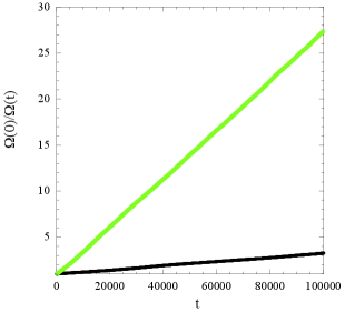
We show in Fig. 1 the time dependence of the rescaled wealth distribution for , starting from the initial condition for all . The wealth disparity between richer and poorer agents initially increases until a steady state is established. Once a steady state is reached, the rescaled wealth distribution remains fixed, and the wealth in every rank increases as .

According to Eq. (1), the growth allocation is weighted more toward the richer agents as , thus leading to a less equal steady state rescaled wealth distribution (see Fig. 2). The time to reach a steady state increases as approaches , and as for , the wealth of all agents increases exponentially after a steady state has been reached. (The limit will always be from below unless otherwise specified.) We find that for , “a rising tide lifts all boats” and all agents benefit from economic growth.

The time-dependence of the rescaled wealth distribution is shown for in Fig. 3. A steady state is not reached, and the slope of the rescaled wealth distribution increases with time, corresponding to the accumulation of wealth by fewer and fewer agents until eventually a single agent gains almost all the wealth. Similar results are found for . The time for a single agent to dominate decreases as increases for .
Note that is a special case for which the increase in an agent’s wealth due to growth is proportional to the agent’s wealth. Hence, for , the ratio of the rescaled wealth of any two agents does not change after the distribution of the growth in wealth according to Eq. (1). Consequently, aside from the exponential growth of the total wealth, the entire dynamics of the system is driven only by the wealth exchange mechanism, and the evolution of the wealth distribution for is identical to its evolution in the original Yard-Sale model; that is, the model with no economic growth.
III Effective ergodicity and economic mobility
The numerical results in Sec. II indicate that the GED model exhibits distinct behavior for and . In particular, for , all agents benefit from economic growth, whereas for only the richest agent becomes richer. In Sec. III.1 we show that the GED model is effectively ergodic for , but is not ergodic for . In Sec. III.2 we find that the agents have nonzero economic mobility for , but have zero mobility for . Unlike in Sec. II, we randomly assign the wealth of each agent at from a uniform distribution and then rescale the agents’ wealth so that the initial total wealth equals .
III.1 Effective ergodicity
To determine whether the system is effectively ergodic, we define the (rescaled) wealth metric as [29]
| (3) |
where is the time averaged wealth of agent at time ,
| (4) | ||||
| (5) | ||||
The metric in Eq. (3) is a measure of how the time averaged wealth of each agent approaches the wealth averaged over all agents. If the system is effectively ergodic, [29]. Effective ergodicity is a necessary, but not a sufficient condition for ergodicity.
The linear time-dependence of shown in Fig. 4(a) for implies that the system is effectively ergodic for . In contrast, for does not increase linearly with [see Fig. 4(b)], and hence the system is not ergodic. Similar results are found for .

III.2 Economic mobility
In a system with economic mobility, poorer agents can become wealthier and richer agents can become poorer. In contrast, agents in a system with very low economic mobility rarely change their rank and the very rich become richer [30].
To determine the mobility, we rank the agents according to their wealth at various times and compute the correlation function of the ranks of the agents once a steady state has been reached for . The rank correlation function of agent is defined as
| (6) |
where is the rank of agent at time and . The corresponding quantity for , where a steady state is not reached, is the Pearson correlation function given by [31]
| (7) |
The correlation function averaged over all agents is . As can be seen from Fig. 5(a), as for , which indicates that the rank of an agent as is not correlated with its rank at and the agents have a nonzero economic mobility for . The dependence of the average time that the richest agent remains the richest is discussed in Sec. VI. In contrast, in Fig. 5(b) we see that approaches a constant for , indicating that the ranks are strongly correlated at different times, and there is no economic mobility.


IV Equilibrium, not just steady state
We have seen that the GED model approaches a steady state and is effectively ergodic for . In the following, we will show that a reasonable definition of the total energy yields an energy distribution that is consistent with the Boltzmann distribution. The existence of the latter is consistent with the idea that that the system is not just in a steady state, but is in thermodynamic equilibrium for .
As discussed in Ref. [28] (following paper), a mean-field theory treatment of the GED model yields a quantity that can be interpreted as the total energy of the system at time
| (8) |
Note that the energy is zero if all agents have the same wealth (). Equation (8) yields a mean energy that is extensive, that is, for fixed values of , , and . For example, for , , and , we find that .
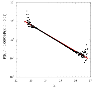
The probability density is shown in Fig. 6(a) for , , , and . As expected, is fit well by a Gaussian. Fits of to a Gaussian become less robust as for fixed , , and . We will discuss the behavior of for larger values of in Sec. V.2.
If the system is in thermodynamic equilibrium, we expect that the probability density to be proportional to , where is an effective inverse temperature that depends on , , and , and is the density of states, which is independent of , , and and hence independent of . Because is independent of , the ratio is an exponential proportional to if the system is characterized by the Boltzmann distribution with the energy given by Eq. (8). The range of values of over which this ratio is nonzero and finite is limited by the overlap of the two probabilities, which becomes smaller as is increased. In Fig. 6(b) we see that the ratio is consistent with the Boltzmann distribution for , , and , with , and ; a larger value of (for fixed values of and ) corresponds to a smaller value of and hence a higher value of the effective temperature. The dependence of the effective temperature on is consistent with the association of with the presence of both additive and multiplicative noise in the system [28]. Similar results hold for two similar values of for fixed and . The existence of an energy, and the observation that its probability is proportional to the Boltzmann distribution implies that the system can be considered to be in thermodynamic equilibrium, at least for .

V Characterization of the phase transition
V.1 Fixed number of agents
The numerical results discussed in this section are for , , and . Averages are taken over a time of ( exchanges) after a transient time of . The major source of uncertainty in our estimations of the values of the various critical exponents is the choice of the range of values to be retained in the least squares fits.
Because we will characterize the approach to the phase transition at in terms of power laws, it is convenient to define the quantity
| (9) |
and will assume that .
To characterize the phase transition at , we need to identify an order parameter. A common measure of income or wealth inequality is the Gini coefficient [32]. If all agents have the same wealth, . In contrast, if one agent has all the wealth, , corresponding to the maximum degree of inequality. These characteristics appear to make a reasonable choice of the order parameter. However, because the wealth distribution reaches a steady state for , the fluctuations of the Gini coefficient are zero in the limit , and hence the susceptibility, which would be associated with the variance of , would be zero, making an inappropriate choice of the order parameter.
The order parameter and the value of . Another choice of the order parameter is the fraction of the wealth held by all the agents except the richest agent, that is,
| (10) |
where is the wealth of the richest agent. For we find that and depends weakly on for fixed values of , , and . For example, for and for , with , , and . The weak dependence of on implies that defined in Eq. (10) approaches one as for independently of the value of (see Fig. 7). Hence, the value of the critical exponent associated with the order parameter is . We also point out that for , the order parameter is zero in the limit . If this branch is continued to , will remain zero (because all agents except the richest have zero wealth), indicating that there is hysteresis. This behavior of raises the question of the order of the transition at . One possibility is that the transition is a spinodal [33].

The susceptibility and the value of . The -dependence of the variance of is shown in Fig. 8(a) and can be fit to a power law to give an effective exponent for the susceptibility close to one for ; fits for smaller values of give an effective exponent approximately equal to 1.7. Both estimates indicate that the variance of the wealth of the richest agent diverges strongly, and hence we choose the order parameter to be as defined in Eq. (10).
More consistent results for the susceptibility can be found from , the variance of the wealth of a single agent averaged over all agents, and not just the variance of the wealth of the richest agent. In Fig. 8(b) we see that there is less curvature in the plot of versus , and we find an effective exponent close to one if fits are made for . If values of are included for larger values of , the effective exponent from the least squares fits is in the range . Given these much better fits, we associate the susceptibility with :
| (11) |
and conclude that the critical exponent associated with the susceptibility is .


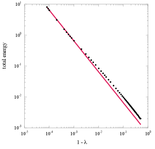
The mean energy, heat capacity, and the value of . Although the total rescaled wealth is a constant, the energy depends on the way the wealth is distributed. We use Eq. (8) to determine the mean energy by averaging the quantity over many realizations. Our results for the mean energy are shown in Fig. 9(a). We see that the -dependence of is consistent with as with . This divergence of is inconsistent with equilibrium statistical mechanics, which requires that the total energy be finite for finite values of .

We define the heat capacity to be the variance of the total energy defined in Eq. (8). The -dependence of of is consistent with the dependence with the exponent as shown in Fig. 9(b). Our determination of the value of depends on the range of values of that are included in the least squares fits and are in the range .
In summary, our numerical results for the critical exponents , , and , determined as is varied for a given value of are consistent with
| (12) |
These numerical values are inconsistent with the usual scaling law
| (13) |
However, the value of determined from the power law behavior of the heat capacity is consistent with the -dependence of the mean total energy, that is, .
V.2 Mean-field theory and fixed Ginzburg parameter
Although it is natural to determine the critical behavior of the GED model as the critical point is approached for a fixed number of agents, our numerical results for the critical exponents are not consistent with the scaling law, Eq. (13), nor consistent with equilibrium statistical mechanics because the mean energy per agent diverges as the critical point is approached even for finite values of and fixed values of and . Simulations also show that and the heat capacity are proportional to for fixed values of , , and so that the divergent behavior of is not removed by first taking the limit before taking the limit .
In Ref. [28] (following paper) a mean-field treatment of the GED model is developed based on the random exchange of wealth between an agent chosen at random and an agent whose wealth is assigned to be equal to the mean wealth of the remaining agents. The mean-field treatment predicts that the critical exponents are given by
| (14) |
The predicted mean-field values of the exponents in Eq. (14) are consistent with Eq. (13). The mean-field theory [28] also predicts that the mean energy per agent approaches a constant as .
To compare the mean-field predictions with the simulations for different values of we need to account for the fact and are rates and depend on the definition of the unit of time. It is shown in the mean-field theory of Ref. [28] that to achieve a consistent thermodynamic description of the GED model, we need to rescale and as we change so that
| (15) |
Another condition for the applicability of the mean-field treatment of the GED model is that the Ginzburg parameter , defined as
| (16) |
be much greater than one and be held fixed as . As has been found for the long-range and fully connected Ising models [33, 34, 35], we will find that the mean-field theory predictions for the critical behavior of the energy and heat capacity of the GED model are consistent with equilibrium statistical mechanics only if the Ginzburg parameter is held fixed as the critical point is approached. We will also see that the results for and do not depend on keeping fixed as has been found for other fully connected models [33, 34, 35].
We emphasize that if and are not rescaled in the simulations, the energy per agent would diverge as even for fixed Ginzburg parameter.
To compare the mean-field theory predictions to the simulations, we choose , , and , with and . For a particular choice of the value of , we determine the value of needed to keep the value of in Eq. (16) fixed at . Our simulations are for and .
Because our results for and depend on keeping fixed, we first discuss their dependence. In Fig. 10 we see that approaches a constant as , in contrast to its divergent behavior for fixed , , and . Because , we find that simulations for fixed Ginzburg parameter are consistent with .

Our numerical results for are consistent with the relation
| (17) |
Equation (17) is predicted by mean-field theory [28] for fixed . For fixed , Eq. (17) implies that approaches a constant as , consistent with our simulations. In contrast, for fixed , , and we find
| (18) |
where and . Equation (18) implies that for fixed values of , , and , is proportional to and diverges as for fixed values of , , and ; both behaviors are consistent with our simulations.
The -dependence of , the variance of the total energy, for fixed is shown in Fig. 11. We see that , with , consistent with the prediction of mean-field theory [28].

Our numerical results for the variance of the total energy are consistent with the relation
| (19) |
For fixed , we have and hence and . For fixed values of and we have
| (20) |
In this case and is proportional to for fixed values of , , and , consistent with the simulations.
The dependence of for fixed is consistent with the mean-field prediction in Ref. [28]. Note that the variance of the total energy is proportional to for fixed , and , but is independent of for fixed Ginzburg parameter. This seemingly inconsistent dependence on is due to the dependence of on for fixed Ginzburg parameter. This confusion is a consequence of the fully connected nature of the GED model. (Recall that an agent can exchange wealth with equal probability with any other agent in the system.) If the mean-field limit is taken according to the prescription of Kac et al. [36], then the agents would be placed, for example, on a two-dimensional lattice and the range over which the agents could exchange wealth would be finite [37]. In this case the Ginzburg parameter would be a function of rather than , and the specific heat would be the heat capacity divided by .
The dependence of the variance of the total energy near implies that the mean energy must include a logarithmic dependence on . For example, the form, , implies that scales as with a logarithmic correction. Mean-field theory is incapable of finding logarithmic corrections, and our data for is not sufficiently accurate to detect the presence of logarithmic factors.
Although our numerical results for depend on whether or is held fixed as , our results for the order parameter and susceptibility exponents and are independent of the nature of the approach to the phase transition. We find that and is independent of for fixed . Hence for , implying that as was found for fixed . The divergence of the susceptibility shown in Fig. 12(b) is consistent with with .

VI Critical slowing down
We find that various time scales increase rapidly as , which limits how close the simulations can approach the transition. One time scale of interest is , the mean lifetime of the richest agent. We expect that if the mobility of the agents is nonzero, then the richest agent at will no longer be the richest after some time has elapsed. We define as the mean time that a particular agent remains the richest and assume that is a simple measure of the decorrelation time of the wealth of individual agents.
Another time scale of interest is the mixing time associated with the time-dependence of the wealth metric; is related to the inverse slope of the wealth metric as
| (21) |
We also computed the time-displaced energy autocorrelation function given by
| (22) |
where is the value of the energy of the system at time . We find that relaxes exponentially, and hence we can extract the energy decorrelation time . Our simulation results for these various times are for fixed Ginzburg parameter ().
For fixed the simulation results for the -dependence of are shown in Fig. 13(a) and are consistent with the power law . To obtain accurate results for the wealth metric , we averaged over ten origins and found that the linear dependence of holds over a wide range of and yields robust values of . The exponential dependence of holds for , yielding some uncertainty in the fitted values of . The -dependence of and are shown in Fig. 13(b). We see that both and increase rapidly as and that their -dependence is consistent with .
Although the mean-field theory [28] makes no direct predictions for the mixing time, the -dependence of can be understood by noting that the metric measures the time it takes for the average wealth of each agent to equal the global average. Because the time it takes for the richest agent to cease being the richest and for another agent to assume that role diverges as approximately , the time for a system of agents to mix is . Because for fixed [see Eq. (16)], we find that in agreement with the simulations.


The mean-field theory of Ref. [28] predicts that the decorrelation time for fixed scales as
| (23) |
The reason for the apparent discrepancy between the -dependence predicted by Eq. (23) and our simulation results for and is that the time unit in the simulations corresponds to exchanges, during which one agent exchanges wealth with only one agent on the average. In contrast, the applicability of mean-field theory requires that in one time unit, one agent exchanges wealth with agents on the average. Hence, the simulation and mean-field time units differ by a factor of or for fixed Ginzburg parameter.
The divergent behavior of and are examples of critical slowing down, which is associated with a cooperative effect and is not a property of a single agent. In contrast, is a property of a single agent rather than of the system as a whole and becomes independent of if we define the time as required by the applicability of mean-field theory.
Although the results of our simulations are consistent with the -dependence in Eq. (23) for constant Ginzburg parameter, Eq. (23) also predicts that is independent of the values of and . As discussed in Ref. [28], the derivation of Eq. (23) neglects the effects of both additive and multiplicative noise. The weak dependence of and on and , as well as their dependence on , is discussed in Ref. [28].
VII Discussion
We have generalized the Yard-Sale model to incorporate economic growth and its distribution according to the wealth of the agents as determined by Eq. (1) and the parameter . Our numerical results suggest that there are two phases. For the system reaches a steady state with economic mobility, is effectively ergodic, and can be considered to be in thermodynamic equilibrium. In contrast, for there is no economic mobility, the system does not reach a steady state, and in the limit , there is condensation of a finite fraction of the system’s wealth in a vanishingly small number of agents. In addition, the system is not ergodic and shares some of the characteristics of the geometric random walk which is also not ergodic and cannot be treated by equilibrium methods [4, 38].
It is remarkable that it is possible to define a thermodynamic energy for a system that involves wealth and has no obvious energy analogue. The interpretation of the energy and its variance is subtle and thermodynamic consistency is achieved only if the mean-field limit is taken appropriately.
We showed in Sec. IV that , the probability density of the energy of the system, is well fit by a Gaussian function for and . Simulations for and values of much closer to one show departures from a Gaussian, even though the wealth fluctuation metric still indicates that the system is effectively ergodic. The deviation of from a Gaussian for fixed (and fixed and ) is due to the fact that decreases as and eventually becomes too small for mean-field theory to be applicable. Simulations for fixed Ginzburg parameter begin to show deviations from a Gaussian distribution for much closer to one. Although the Ginzburg parameter is large and fixed, the importance of multiplicative noise increases as , and eventually the effect of the multiplicative noise can no longer be ignored [28].
Our numerical values of the various exponents are consistent with the mean-field theory of Ref. [28], but their estimated numerical values must be viewed with caution because they are obtained by extrapolation over a limited range of and for finite values of and . Much larger values of would be needed to obtain more accurate numerical results for closer to one.
The transition at is from a system in thermodynamic equilibrium for to a system that undergoes wealth condensation for . In Ref. [28] it is shown that the evolution of the model for is the same as unstable state evolution in the fully connected Ising model for model A dynamics [39]. In Fig. 14 we show the evolution of the wealth of the richest agent after the value of has been changed from to and to . We see that the wealth of the richest agent initially increases exponentially. We also find that the duration of exponential growth decreases for larger values of after the change (not shown).

Our results have possible important economic implications. As is increased, the benefits of growth are weighted more toward the wealthy, and wealth inequality increases. Nevertheless, as long as , the wealth of agents of all ranks grows at the same rate once a steady state is reached, and all agents benefit from economic growth. However, if the benefits of growth are skewed too much toward the wealthy (), poor and middle rank agents no longer benefit from economic growth, and wealth condensation occurs. For the model reduces to the geometric random walk with resulting wealth condensation [4], as shown in the following paper [28].
There is some question whether economic systems can be treated as being in equilibrium or even exhibit effective ergodicity [4, 38, 10]. Our results suggest that ergodicity and equilibrium may depend on various system parameters. Because parameters such as and are not temporal constants in real economies, our results also suggest that the applicability of equilibrium methods may be situational and vary with time.
Acknowledgements.
We thank Timothy Khouw, Ole Peters, John Ogren, Alan Gabel, Bill Gibson, Karen Smith, and Louis Colonna-Romano for useful conversations.*
Appendix A Comparison to some economic data
Modeling the economy of a country as large and diverse as the United States by compressing economic growth and transactions into three parameters, , , and is a gross simplification. The assumption that these parameters are independent of time also is unrealistic. In the following, we analyze the growth data [40] and wealth distribution data [41] compiled by Karen Smith and published by the Urban Institute. Our analysis suggests that the assumptions that the distribution of growth can be modeled as in Eq. (1) and that the parameters are independent of time is a reasonable zeroth order approximation to the distribution of wealth in the real economy. We will discuss the exchange term and its relevance to the real economy in the following paper [28].
From the growth rate of the gross domestic product shown in constant dollars in Ref. [40], we note that the temporal fluctuations of the (inflation adjusted) growth rate of the gross domestic product exhibits large swings that appear to be damped as a function of time. The decline in the growth caused by the great recession starting in 2008 is an example of a large fluctuation, but the growth rate has remained close to the mean rate of roughly 3% over the last 30 years, thus implying that .
By using the wealth distribution chart in Ref. [41], we can calculate the change of the wealth of people in various percentiles. From the relation [see Eq. (1)], we can estimate as
| (24) |
where is the wealth of people of economic rank (percentile) at time .
We estimated for the 50th, 90th and 95th wealth percentiles in the intervals 1983–1989, 1995 –1998 and 2013–2016 (see Table 1). Although the values of are not constant for different time intervals and percentiles, they vary by only a few percentage points as a function of percentile. They vary more as a function of time, with the 50% percentile having the greatest variation. The change of appears to decrease for later times, consistent with the damping of the variation of the growth. The variation of is more pronounced for even lower rankings. However, because the wealth of the lower rankings is considerably smaller, the variation of the value of has less effect on the wealth of the poor.
| percentile | 1983–1989 | 1995–1998 | 2013–2016 |
|---|---|---|---|
| 95% | 0.85 | 0.90 | 0.90 |
| 90% | 0.84 | 0.89 | 0.90 |
| 50% | 0.75 | 0.90 | 0.84 |
We conclude from the growth and wealth distribution data [40, 41] that the distribution of economic growth assumed in the GED model is a reasonable zeroth order approximation, particularly for the upper half of the wealth ranks of the United States over the past 30 years. Of course, there is much that it is not included in the model, such as the effects of wars, famines, storms, and recessions, which are not obtainable from the simple GED model. However, it appears from the data that the model is a reasonable approximation over time scales of the order of decades and yields insights into the importance of how economic growth is distributed.
References
- [1] A. Chakraborti, I. M. Toke, M. Patriarca, and F. Abergel, “Econophysics review: II. Agent-based models,” Quant. Finance 11, 1013 (2011).
- [2] J. F. Kennedy, “Remarks in Heber Springs Arkansas at the dedication of the Greers Ferry Dam,” The American Presidency Project, 3 October 1963, <https://www.jfklibrary.org/asset-viewer/archives/JFKPOF/047/JFKPOF-047-015>.
- [3] E. Gudreis, “Unequal America,” Harvard Magazine, July–August (2008).
- [4] O. Peters, “Optimal leverage from non-ergodicity,” Quant. Finance 11, 1593 (2011).
- [5] J. Angle, “The surplus theory of social stratification and the size distribution of personal wealth,” Social Forces 65, 293 (1986).
- [6] J. Angle, “Deriving the size distribution of personal wealth from the rich get richer, the poor get poorer,” J. Math. Sociology 18, 27 (1993).
- [7] A. Chakraborti and B. K. Chakrabarti, “Statistical mechanics of money: how saving propensity affects its distribution,” Eur. Phys. J. B 17, 167 (2000).
- [8] A. Drägulescu and V. M. Yakovenko, “Statistical mechanics of money,” Eur. Phys. J. B 17, 723 (2000).
- [9] C. F. Moukarzel, S. Goncalves, J. R. Iglesias, M. Rodriguez-Achach, and R. Huerta-Quintanilla, “Wealth condensation in a multiplicative random asset exchange model,” Eur. Phys. J.-Spec. Top. 143, 75 (2007).
- [10] V. M. Yakovenko and J. B. Rosser Jr., “Colloquium: Statistical mechanics of money, wealth, and income,” Rev. Mod. Phys. 81, 1703 (2009).
- [11] M. Patriarca and A. Chakraborti, “Kinetic exchange models: From molecular physics to social science,” Am. J. Phys. 81, 618 (2013).
- [12] J.-P. Bouchaud and M. Mézard, “Wealth condensation in a simple model of economy,” Physica A 282, 536 (2000).
- [13] Z. Burda, D. Johnston, J. Jurkiewicz, M. Kamiński, M. A. Nowak, G. Papp, and I. Zahed, “Wealth condensation in Pareto macroeconomies,” Phys. Rev. E 65, 026102 (2002).
- [14] B. M. Boghosian, “Kinetics of wealth and the Pareto law,” Phys. Rev. E 89, 042804 (2014).
- [15] B. M. Boghosian, “Fokker-Planck description of wealth dynamics and the origin of Pareto’s Law,” Int. J. Mod. Phys. C 25, 1441008 (2014).
- [16] B. M. Boghosian, M. Johnson, and J. A. Marcq, “An H theorem for Boltzmann’s equation for the yard-sale model of asset exchange,” J. Stat. Phys. 161, 1339 (2015).
- [17] C. Chorro, “A simple probabilistic approach of the Yard-Sale model,” Statistics and Probability Letters 112, 35 (2016).
- [18] B. M. Boghosian, A. Devitt-Lee, M. Johnson, J. Li, J. A. Marcq, and H. Wang, “Oligarchy as a phase transition: The effect of wealth-attained advantage in a Fokker-Planck description of asset exchange,” Physica A 476, 15 (2017). “Wealth-attained advantage” is implemented by biasing the coin flip for the exchange of wealth in favor of the wealthier agent. In contrast, we implement a form of wealth-attained advantage by an uneven redistribution of wealth due to growth.
- [19] A Devitt-Lee, H. Wang, J. Ii, and B. Boghosian, “A nonstandard description of wealth concentration in large-scale economies,” Siam J. Appl. Math 78, 996 (2018).
- [20] J. Li, B. M. Boghosian, and C. Li, “The affine wealth model: An agent-based model of asset exchange that allows for negative-wealth agents and its empirical validation,” Physica A 516, 423 (2019).
- [21] B. M. Boghosian, “The inescapable casino,” Sci. Amer. 321 (11), 72 (2019).
- [22] P. L. Krapivsky and S. Redner, “Wealth distributions in asset exchange models,” Science and Culture 76, 424 (2010).
- [23] S. Ispolatov, P. L. Krapivsky, and S. Redner, “Wealth distributions in asset exchange models,” J. Eur. Phys. B 2, 267 (1998).
- [24] A. Chakraborti, “Distributions of money in model markets of economy,” Int J. Mod. Phys. C 13, 1315 (2002).
- [25] B. Hayes, “Follow the money,” Am. Sci. 90, 400 (2002).
- [26] F. Slanina, “Inelastically scattering particles and wealth distribution in an open economy,” Phys. Rev. E 69, 046102 (2004). This paper was one of the first to consider increasing wealth, although the exchange mechanism was additive rather than multiplicative.
- [27] The Yard-Sale model and its generalizations incorporate the exchange of wealth not income. The distinction between wealth and income is important in more detailed models of the economy. The distribution of income and wealth show similar trends, but the distribution of wealth is more unequal than the distribution of income. See, for example, M. Cragg and R. Ghayad, “Growing apart: The evolution of income vs. wealth inequality,” The Economists’ Voice 12(1), 1–12 (2005), A. Drägulescu, V. M. Yakovenko, “Exponential and power-law probability distributions of wealth and income in the United Kingdom and the United States,” Physica A 299, 213 (2001), and Y. Berman, E. Ben-Jacob, and Y. Shapira, “The dynamics of wealth inequality and the effect of income distribution,” PLoS ONE 11(4), e0154196 (2016).
- [28] W. Klein, N. Lubbers, K. K. L. Liu, and H. Gould, “Mean-field theory of an asset exchange model with economic growth and wealth distribution,” arXiv:2102.01274.
- [29] D. Thirumalai and R. D. Mountain, “Activated dynamics, loss of ergodicity, and transport in supercooled liquids,” Phys. Rev. A 42, 4574 (1990) and Phys. Rev. E 47, 479 (1993).
- [30] B.-H. F. Cardoso, S. Gonçalves, J. R. Iglesias, “Wealth distribution models with regulations: Dynamics and equilibria,” Physica A 551, 124201 (2020). The authors investigate a modification of the Yard-Sale model that favors the poorer agent (social protection). One consequence is that the agents in their modified Yard-Sale model have economic mobility under certain conditions. The authors also investigate the hysteresis of the wealth distribution due to the removal of social protection.
- [31] J. L. Rodgers and W. A. Nicewander, “Thirteen ways to look at the correlation coefficient,” Amer. Stat. 42, 59 (1988).
- [32] For a discussion of the Gini coefficient, see, for example, <https://en.wikipedia.org/wiki/Gini_coefficient>.
- [33] W. Klein, H. Gould, N. Gulbahce, J. B. Rundle, and K. F. Tiampo, “The structure of fluctuations near mean-field critical points and spinodals and its implication for physical processes,” Phys. Rev. E 75, 031114 (2007).
- [34] L. Colonna-Romano, H. Gould and W. Klein, “Anomalous mean-field behavior of the fully connected Ising model,” Phys. Rev. E 90, 042111 (2014).
- [35] Kang K. L. Liu, J. B. Silva, W. Klein, and H. Gould, “Anomalous behavior of the specific heat in systems with long-range interactions,” manuscript in preparation.
- [36] M. Kac, G. E. Uhlenbeck and P. Hemmer, “On the van der Waals theory of the vapor-liquid equilibrium. I. Discussion of a one-dimensional model,” J. Math. Phys. 4, 216 (1963).
- [37] T. Khouw, W. Klein, and H. Gould, “Globalization and inequality in an agent-based asset exchange model,” manuscript in preparation.
- [38] O. Peters and W. Klein, “Ergodicity breaking in geometric Brownian motion,” Phys. Rev. Lett. 110, 100603 (2013).
- [39] P. C. Hohenberg and B. I. Halperin, “Theory of dynamic critical phenomena,” Rev. Mod. Phys. 49, 435 (1977).
- [40] The U.S. real GDP growth rate adjusted for inflation, https://www.multpl.com/us-real-gdp-growth-rate>.
- [41] Summary of wealth inequality in the U.S., <http://apps.urban.org/features/wealth-inequality-charts/>.