Simulated quantum annealing as a simulator of non-equilibrium quantum dynamics

We study the non-equilibrium dynamics, in particular the properties related to the original [43, 44] and the generalized Kibble-Zurek mechanisms [39, 40], of the ferromagnetic transverse-field Ising model in one dimension with a free boundary,

Here $L$ is the number of sites (qubits), $\hat{\sigma}^{\mu}_{i}~{}(\mu=x,z)$ is the $\mu$ component of the Pauli matrix at site $i$, and $J(t)$ and $\Gamma(t)$ are the time-dependent coefficients for the target and driver terms, respectively. We use the linear time dependence of the coefficients for simplicity,

where $t_{a}$ is the annealing time and the time $t$ runs from 0 to $t_{a}$. This system in the ground state undergoes an equilibrium second-order phase transition at a critical point $J=\Gamma$ in the limit of infinite system size [45].

In addition to the above Hamiltonian representing a closed quantum system, we also study the open system described by the Hamiltonian,

where $V_{k}$ is the coupling constant with the $k$th bosonic mode $\hat{a}^{\dagger}_{i,k}$ and $\hat{a}_{i,k}$ representing the environment, which is assumed to have the standard Ohmic spectral density $J(\omega)=4\pi\sum_{k}{V_{k}}^{2}\delta(\omega-\omega_{i,k})=2\pi\alpha\omega$. Following Ref. [46], we assume $J(\omega)$ to be cutoff at some $\omega_{c}$, beyond which $J(\omega)$ is set to 0. The coefficient $\alpha$ describes the magnitude of dissipation caused by the coupling to the environment. The whole system of Eq. (II.1) is isolated from other degrees of freedom, kept at zero temperature, and in principle running under the unitary Schrödinger dynamics without the constraint of adiabaticity. SQA is supposed to simulate the dynamical behavior of this system.

The problem defined above has been studied extensively for many years. Directly pertinent to the present paper are, first, the path-integral Monte Carlo simulation by Werner et al. [46], who studied the equilibrium phase diagram and critical exponents of the open system of Eq. (II.1), and found that critical exponents are different from those of the closed system, Eq. (1), but are independent of the coupling strength $\alpha(>0)$. Also, Bando et al. [17] carried out experiments on the D-Wave quantum annealers and compared the data with the generalized Kibble-Zurek mechanism [39, 40] to conclude that the data from the devices can be understood in terms of a system under the bosonic environment of Eq. (II.1), not of the closed system Eq. (1), and also that the classical SVMC is unable to explain the dynamical properties of the D-Wave devices.

We combine these two contributions and study the systems of Eqs. (1) and (II.1) by SQA, path-integral Monte Carlo simulations with time-dependent coefficients $J(t)$ and $\Gamma(t)$, and compare the data with those from the generalized Kibble-Zurek mechanism as well as from the more direct numerical method of the iTEBD-QUAPI [42, 41], in which the time-dependent density operator is expressed by a matrix-product state after a Trotter decomposition and tracing out the bosonic degrees of freedom. Then a controlled truncation of basis states allows one to perform evaluation of physical quantities. See Refs. [42, 41] for details.

To perform SQA, we first apply the Suzuki-Trotter decomposition [36] to the expression of the partition function for the Hamiltonian of Eq. (II.1). The partition function is then expressed as the corresponding partition function of a classical Ising model in two dimensions with long-range interactions in the Trotter (imaginary-time) direction [46],

where $Z_{0}$ is the partition function of free bosons and

Here, $\beta_{\rm{eff}}=\beta/P$ with $\beta$ the inverse temperature and $P$ the number of Trotter slices along the imaginary-time axis. The coefficient in the second line is defined as $\gamma(t)=-\frac{1}{2}\ln{[\tanh{(\beta_{\rm{eff}}\Gamma(t))}]}$. A periodic boundary condition $S_{i}({P+1})=S_{i}({1})$ is imposed along the Trotter axis. The closed system of Eq. (1) is recovered by setting $\alpha=0$. Zero-temperature properties of Eq. (II.1) can be simulated with sufficiently large values $\beta$ and $P$ with a fixed finite value of the ratio $\beta_{\rm{eff}}=\beta/P$ [2, 5, 6]. We choose $\beta_{\rm{eff}}=1$ and $P=4L$ to satisfy this condition as described in more detail below.

Although cluster updates have sometimes been used in related studies  [46, 32, 35], we use the simple single-flip Metropolis-update dynamics because, first, it is non-trivial which stochastic dynamics better simulates quantum dynamics, and second, we do not expect to encounter the problem of slow relaxation, which hampers simulations of disordered systems based on simple single-spin updates [35], or we do not need to reach the equilibrium necessary for the study of critical exponents [46]. The annealing time $t_{a}$ is identified with the total number of Monte Carlo steps divided by the number of sites $LP$ and will be denoted by $\tau_{\rm MCS}(=t_{a})$. Values of time-dependent coefficients $J(t)$ and $\Gamma(t)$ are updated according to Eqs. (2) and (3) after a unit time (a Monte Carlo update trial per spin), $t\to t+1$.

Following Ref. [17], we measure several quantities by SQA to be compared with predictions of the generalized Kibble-Zurek mechanism and the iTEBD-QUAPI. All quantities are measured at the end of computation where $\Gamma(t_{a})=0$.

The main quantity of interest is the number of defects (spatially mis-aligned spin pairs) $n$,

Notice that the true ground state of the effective Hamiltonian of Eq. (6) is perfectly ferromagnetic with $n=0$.

We measure the statistics of defects to be denoted by $P^{\rm{SQA}}(n)$ and compare it with the prediction of the generalized Kibble-Zurek mechanism [39, 40]. According to this theory, the defect distribution is bimodal and is well approximated by the Gaussian function $Q(n)$ for large systems $L\gg 1$,

where $\kappa_{1}\equiv\langle n\rangle$ and $\kappa_{2}\equiv\langle(n-\langle n\rangle)^{2}\rangle$. Here angular brackets $\langle\cdots\rangle$ denote the average. We quantify the difference between $P^{\rm{SQA}}(n)$ and $Q(n)$ by the $L1$ norm,

We also follow Ref. [17] and check the proximity of $P^{\rm{SQA}}(n)$ to the Boltzmann distribution of the classical Ising part of the original Hamiltonian in Eq. (1),

where $E(n)$ is the energy of the classical Ising model with $n$ defects. We optimize the effective inverse temperature $\beta_{\rm{BL}}$ in $P^{\rm{BL}}(n)$ by minimizing the $L1$ norm of Eq. (9) (after replacing $Q(n)$ with $P^{\rm{BL}}(n)$) such that $P^{\rm{BL}}(n)$ approximates $P^{\rm{SQA}}(n)$ as faithfully as possible. Notice that $\beta_{\rm{BL}}$ is unrelated to any physical temperature but is a parameter to fit Eq. (II.3) to the data.

The number of defects $n$ in Eq. (7) is essentially equivalent to the residual energy per site $E_{\rm{res}}$, the difference between the achieved energy and the true ground-state energy, for which we use the expression of Ref. [35],

Note that $E_{\rm{res}}$ can also be regarded as the average number of defects, the average over the statistics of $P^{\rm SQA}(n)$, which was denoted by $\kappa_{1}$ (the first cumulant or the average) above.

The data for $E_{\rm{res}}$ are to be compared with the predictions of the Kibble-Zurek mechanism, which is described qualitatively as follows. As the system approaches a critical point, the correlation length and relaxation time grow rapidly. When the system is not close enough to the critical point, the relaxation time is large but still shorter than the time scale of annealing, and the system has time to relax to equilibrium. As the system comes closer to the critical point, the relaxation time becomes long enough and the system has no time to relax and is effectively frozen with a non-vanishing residual energy. This picture leads to the asymptotic power law of the residual energy [47],

Here, $d=1$ is the spatial dimension and $z$ and $\nu$ are the dynamical and correlation-length critical exponents, respectively.

We first report the results for the closed system of Eq. (1). Figure 1 shows the residual energy $E_{\rm{res}}$ defined in Eq. (11) as a function of the annealing time $\tau_{\rm{MCS}}$ for system sizes $L=64,128,256$, and $512$. We set $\beta_{\rm eff}=\frac{\beta}{P}=1$ and $P=4L$. As shown in Appendix A, we have confirmed that the residual energy as a function of $P$ converges for $P=4L$. This condition is used throughout this paper.

It is clearly shown in Fig. 1 that the residual energy follows a power law as predicted by the original Kibble-Zurek mechanism,

The values of the exponent $b$ are found as $b=0.543\pm 0.007~{}(L=64)$, $0.519\pm 0.004~{}(L=128)$, $0.506\pm 0.003~{}(L=256)$, and $0.500\pm 0.003~{}(L=512)$. These values, particularly the last one, are in close agreement with the prediction of the Kibble-Zurek mechanism Eq. (12) for this one-dimensional closed system, which has $z=1$, $\nu=1$, and thus $b=d\nu/(1+z\nu)=\frac{1}{2}$. This agrees with previous reports by the direct numerical method of the i-TEBD-QUAPI  [41, 42] as well as by SQA [32, 35]. By contrast, as found in Ref. [17], the SVMC shows close, but slightly deviated, values $b=0.477\pm 0.005$ and $b=0.482\pm 0.006$, depending on the choice of the simulation temperature, 12.1 mK for the former value corresponding to the device at NASA Ames Research Center and 13.5 mK for the latter value for the device at Burnaby.

We proceed to the analysis of the distribution function of defects $P^{\rm SQA}(n)$. Figure 2 shows the $q$th cumulants $\kappa_{q}~{}(q=1,2,3)$ of the defect distribution obtained from the final state at $\tau_{\rm MCS}$ of SQA for $L=64,128,256$, and $512$.

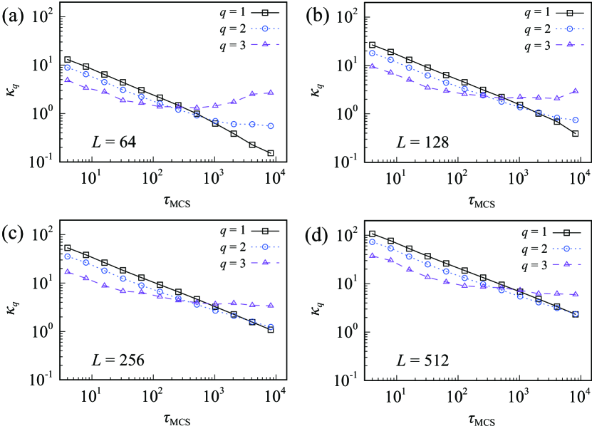
The generalized Kibble-Zurek mechanism [39, 40] predicts that the second- and higher-order cumulants are proportional to the first-order cumulant (average) $\kappa_{1}$. The data shows that this is indeed the case for $\tau_{\rm{MCS}}$ up to about $10^{2}$ for any system size $L$ but the tendency changes beyond $\tau_{\rm MCS}\approx 10^{2}$. Comparison of data for different system sizes suggests that this deviation may possibly be a finite-size effect.

Figure 3 shows the ratios of cumulants $\kappa_{2}/\kappa_{1}$ and $\kappa_{3}/\kappa_{1}$ for $\tau_{\rm MCS}$ up to about $10^{2}$ for $L=512$, which indicates the validity of proportionality of $\kappa_{2}$ and $\kappa_{3}$ to $\kappa_{1}$ up to $\tau_{\rm MCS}\approx 10^{2}$. More quantitatively, we find $\kappa_{2}/\kappa_{1}=0.688\pm 0.005$ and $\kappa_{3}/\kappa_{1}=0.394\pm 0.019$. These values clearly deviate from the theoretical prediction for the closed system, $\kappa_{2}/\kappa_{1}=0.578$ and $\kappa_{3}/\kappa_{1}=0.134$ [39, 40]. We therefore conclude that SQA does not faithfully reproduce the statistics of the defect distribution for the present closed system although the average or the residual energy is well described by SQA.

It may be useful to recall in passing that the data from the D-Wave devices showed similar proportionality but with values closer to the theory, $\kappa_{2}/\kappa_{1}=0.61\pm 0.03$ and $\kappa_{3}/\kappa_{1}=0.23\pm 0.15$ on the device at NASA and $\kappa_{2}/\kappa_{1}=0.63\pm 0.05$ and $\kappa_{3}/\kappa_{1}=0.25\pm 0.18$ on the device at Burnaby [17]. In contrast, the SVMC data marginally indicate proportionality of $\kappa_{2}$ to $\kappa_{1}$ in the short time region but with significant deviations for longer annealing times [17]. The ratio $\kappa_{2}/\kappa_{1}$ out of SVMC is close to 0.6 for the short-time region but the ratio $\kappa_{3}/\kappa_{1}$ has large error bars and it is impossible to determine its value with reliability.

We further follow Ref. [17] and test if the defect distribution is closer to the Boltzmann or Gaussian distribution. Figure 4 is the distribution function at $\tau_{\rm{MCS}}=16,256$, and $4096$ and the dashed line is the Boltzmann distribution Eq. (II.3) with the effective inverse temperature $\beta_{\rm{BL}}$ optimized for each $\tau_{\rm{MCS}}$.

Though the data appears to be close to the optimized Boltzmann distribution $P^{\rm{BL}}(n)$, we see a slight deviation especially at $\tau_{\rm{MCS}}=16$, which is more clearly observed in the enhanced figure in Fig. 5, where we see a better fit by the Gaussian Eq. (8), similarly to the previous study by the D-Wave devices and SVMC [17].

Figure 6 shows the L1 norm of the difference between the defect distribution of SQA, $P^{\rm{SQA}}(n)$, and the optimized Boltzmann distribution $P^{\rm BL}(n)$ in Eq. (II.3) and the Gaussian distribution $Q(n)$ in Eq. (8) as a function of the annealing time $\tau_{\rm{MCS}}$ for $L=512$. In the time range up to $\tau_{\rm{MCS}}\approx 10^{2}$, where the proportional relationship of cumulants is established, the L1 norm with the Gaussian is smaller, and thus SQA works as a Gaussian sampler rather than as a Boltzmann sampler, but for longer annealing times, e.g., $\tau_{\rm{MCS}}\approx 10^{3}$, two functions show similar degrees of proximity to the data.

Those results for the closed system indicate that the classical stochastic dynamics of SQA partly succeeds in reproducing the predictions on the quantum dynamics related to the original and generalized Kibble-Zurek mechanism. However, detailed quantitative analysis of the distribution function show deviations from the theory for the closed system.

We next discuss the results obtained for the open system defined in Eq. (II.1) and simulated by Eq. (6).

Figure 7 shows the residual energy $E_{\rm{res}}$ as a function of $\tau_{\rm{MCS}}$ for $L=64,128,256$, and $512$ under the same parameters as before, $\beta_{\rm eff}=\frac{\beta}{P}=1$ and $P=4L$. Here, we fix the coupling strength with the boson field to $\alpha=0.6$ for all $L$.

It is seen that the power decay predicted by the Kibble-Zurek mechanism, Eq. (13), holds up to $\tau_{\rm MCS}\approx 10^{3}$. Deviations are observed even for the largest system with $L=512$ beyond this annealing time in contrast to the case of the closed system in Fig. 1. It is anticipated from the behavior beyond $\tau_{\rm MCS}\approx 10^{3}$ that these deviations may be due to finite-size effects. Quantitatively, the exponents extracted from the linear region are $b=0.433\pm 0.013,0.437\pm 0.006,0.431\pm 0.008$, and $0.425\pm 0.007$ for $L=64,128,256$, and $512$, respectively, indicating deviations from the closed-system value $b=0.5$. Critical exponents $z=1.985$ and $\nu=0.638$ from equilibrium Monte Carlo simulation of the open system in Ref. [46] lead to $b=d\nu/(1+z\nu)=0.28$. Our estimate $b\approx 0.43$ from SQA with $\alpha=0.6$ is not close to either of those theoretical values 0.5 and 0.28 for closed and open systems, respectively.

Extensive numerical simulations of open quantum systems by the i-TEBD-QUAPI, which is expected to faithfully reproduce quantum dynamics for the very short-time region, showed clear dependence of the exponent $b$ on several factors including the coupling strength $\alpha$ and the range of annealing time [41, 42, 17]. We therefore checked the $\alpha$-dependence of the residual energy by SQA, and the result is in Fig. 8 for $L=256$. It is seen that the exponent $b$ is a decreasing function of $\alpha$ (from $b=0.50$ for $\alpha=0$ to $b=0.26$ for $\alpha=1.0$), consistently with the results of i-TEBD-QUAPI reported in Refs. [17, 41, 42]. For the reader’s convenience, we reproduce a figure from Ref. [17] as Fig. 15 of Appendix B of this paper, where the defect density (proportional to the residual energy) is drawn as a function of the annealing time. One observes there that $b$ changes from $b=0.50$ for $\alpha=0$ to $b=0.25$ for $\alpha=1.28$, close to the values from SQA.

As suggested in Ref. [17], taking into account the fact that the i-TEBD-QUAPI reproduces quantum dynamics for very short times, this non-universality (dependence of the exponent on $\alpha$) of the SQA data may imply that the system is still in a transient state and much longer annealing times for much larger systems may show a value of $b$ independent $\alpha$ as expected from universality seen in the equilibrium Monte Carlo simulation [46]. Viewed differently, this consistency with the quantum-mechanical simulation by the i-TEBD-QUAPI may imply that SQA, a classical stochastic process, reproduces some aspects of the non-equilibrium quantum dynamics in the short time region for the present open system.

We proceed to test if the distribution function of defects $P^{\rm SQA}(n)$ for a typical fixed value of $\alpha=0.6$ is consistent with the prediction of the generalized Kibble-Zurek mechanism as we did for the closed system. Figure 9 shows the $q$th cumulants of the distribution as functions of the annealing time for $L=64,128,256$, and $512$. It is seen that the second cumulant is proportional to the first cumulant almost up to $\tau_{\rm MCS}\approx 10^{3}$, a longer time range of proportionality than in the closed system depicted in Fig. 2. The behavior of the third cumulant is unstable due to insufficient statistics.

Figure 10 shows the ratios of cumulants with the results $\kappa_{2}/\kappa_{1}\approx 0.598\pm 0.008$ and $\kappa_{3}/\kappa_{1}\approx 0.185\pm 0.048$. These values for the open system are closer to the theoretical prediction of the generalized Kibble-Zurek mechanism ($\kappa_{2}/\kappa_{1}=0.578$ and $\kappa_{3}/\kappa_{1}=0.174$ [40]) than in the case of SQA for the closed system discussed in the preceding section ($\kappa_{2}/\kappa_{1}\approx 0.688\pm 0.005$ and $\kappa_{3}/\kappa_{1}\approx 0.394\pm 0.019$). We have also calculated cumulant ratios with a different coupling strength $\alpha=1.0$ in $L=512$ to see the $\alpha$ dependence. The result is $\kappa_{2}/\kappa_{1}\approx 0.569\pm 0.015$ and $\kappa_{3}/\kappa_{1}\approx 0.196\pm 0.135$, indicating very weak dependence on $\alpha$.

It was found in Ref. [17] that the numerical data by the i-TEBD-QUAPI for the open system indicate a similar value 0.6 for $\kappa_{2}/\kappa_{1}$ independent of $\alpha$ but it is difficult to evaluate $\kappa_{3}/\kappa_{1}$. We have thus found that SQA for the open system successfully reproduces the prediction of the generalized Kibble-Zurek mechanism for the cumulant ratios, but the behavior of the average (residual energy) is non-universal, which is not compatible with the theory. Also, agreement with the data of the iTEBD-QUAPI in the short time region has been observed.

As in the case of the closed system, we further check whether the distribution function is closer to the Gaussian or Boltzmann. Figure 11 shows the distribution function for $\tau_{\rm{MCS}}=16,256$, and 4096 for $L=512$ with the coupling constant $\alpha=0.6$ fitted to the Boltzmann distribution Eq. (II.3) with optimized effective temperature.

Although the gross feature is captured by the Boltzmann distribution, we find clear deviations. In fact, as seen in Fig. 12, the Gaussian distribution better matches the data, as anticipated from the smallness of the third cumulant.

Figure 13 shows the L1 norm between the defect distribution of SQA, $P^{\rm{SQA}}(n)$, and the optimized Boltzmann distribution $P^{\rm BL}(n)$ in Eq. (II.3) and the Gaussian distribution $Q(n)$ of Eq. (8) as a function of the annealing time $\tau_{\rm{MCS}}$ for $L=512$. It is seen that the data is closer to the Gaussian distribution than to the Boltzmann, similarly to the case of the closed system and in agreement with the generalized Kibble-Zurek mechanism which predicts small values of higher-order cumulants than the second order, meaning Gaussian approximately. Thus SQA is closer to a Gaussian sampler rather than a Boltzmann sampler in the present open system as well. A similar conclusion was drawn for the D-Wave device [17], and therefore we should be careful when we use quantum annealing (simulated or on the real device) for sampling purposes at least as long as the present one-dimensional system is concerned.

References

- Kadowaki and Nishimori [1998] T. Kadowaki and H. Nishimori, Quantum annealing in the transverse ising model, Phys. Rev. E 58, 5355 (1998).
- Kadowaki [1998] T. Kadowaki, Study of Optimization Problems by Quantum Annealing, Ph.D. thesis, Tokyo Institute of Technology (1998), arXiv:0205020 .
- Brooke et al. [1999] J. Brooke, D. Bitko, T. F. Rosenbaum, and G. Aeppli, Quantum annealing of a disordered magnet, Science 284, 779 (1999).
- Farhi et al. [2001] E. Farhi, J. Goldstone, S. Gutmann, J. Lapan, A. Lundgren, and D. Preda, A quantum adiabatic evolution algorithm applied to random instances of an NP-complete problem., Science 292, 472 (2001).
- Santoro et al. [2002] G. E. Santoro, R. Martoňák, E. Tosatti, and R. Car, Theory of quantum annealing of an ising spin glass, Science 295, 2427 (2002).
- Santoro and Tosatti [2006] G. E. Santoro and E. Tosatti, Optimization using quantum mechanics: quantum annealing through adiabatic evolution, J. Phys. A 39, R393 (2006).
- Das and Chakrabarti [2008] A. Das and B. K. Chakrabarti, Colloquium: Quantum annealing and analog quantum computation, Rev. Mod. Phys. 80, 1061 (2008).
- Morita and Nishimori [2008] S. Morita and H. Nishimori, Mathematical foundation of quantum annealing, J. Math. Phys. 49, 125210 (2008).
- Albash and Lidar [2018] T. Albash and D. A. Lidar, Adiabatic quantum computation, Rev. Mod. Phys. 90, 015002 (2018).
- Hauke et al. [2020] P. Hauke, H. G. Katzgraber, W. Lechner, H. Nishimori, and W. D. Oliver, Perspectives of quantum annealing: Methods and implementations, Rep. Prog. Phys. 83, 054401 (2020).
- Harris et al. [2018] R. Harris, Y. Sato, A. J. Berkley, M. Reis, F. Altomare, M. H. Amin, K. Boothby, P. Bunyk, C. Deng, C. Enderud, S. Huang, E. Hoskinson, M. W. Johnson, E. Ladizinsky, N. Ladizinsky, T. Lanting, R. Li, T. Medina, R. Molavi, R. Neufeld, T. Oh, I. Pavlov, I. Perminov, G. Poulin-Lamarre, C. Rich, A. Smirnov, L. Swenson, N. Tsai, M. Volkmann, J. Whittaker, and J. Yao, Phase transitions in a programmable quantum spin glass simulator, Science 361, 162 (2018).
- King et al. [2018] A. D. King, J. Carrasquilla, J. Raymond, I. Ozfidan, E. Andriyash, A. Berkley, M. Reis, T. Lanting, R. Harris, F. Altomare, K. Boothby, P. I. Bunyk, C. Enderud, A. Fréchette, E. Hoskinson, N. Ladizinsky, T. Oh, G. Poulin-Lamarre, C. Rich, Y. Sato, A. Y. Smirnov, L. J. Swenson, M. H. Volkmann, J. Whittaker, J. Yao, E. Ladizinsky, M. W. Johnson, J. Hilton, and M. H. Amin, Observation of topological phenomena in a programmable lattice of 1,800 qubits, Nature 560, 456 (2018).
- King et al. [2021a] A. D. King, J. Raymond, T. Lanting, S. V. Isakov, M. Mohseni, G. Poulin-Lamarre, S. Ejtemaee, W. Bernoudy, I. Ozfidan, A. Y. Smirnov, M. Reis, F. Altomare, M. Babcock, C. Baron, A. J. Berkley, K. Boothby, P. I. Bunyk, H. Christiani, C. Enderud, B. Evert, R. Harris, E. Hoskinson, S. Huang, K. Jooya, A. Khodabandelou, N. Ladizinsky, R. Li, P. A. Lott, A. J. R. MacDonald, D. Marsden, G. Marsden, T. Medina, R. Molavi, R. Neufeld, M. Norouzpour, T. Oh, I. Pavlov, I. Perminov, T. Prescott, C. Rich, Y. Sato, B. Sheldan, G. Sterling, L. J. Swenson, N. Tsai, M. H. Volkmann, J. D. Whittaker, W. Wilkinson, J. Yao, H. Neven, J. P. Hilton, E. Ladizinsky, M. W. Johnson, and M. H. Amin, Scaling advantage in quantum simulation of geometrically frustrated magnets, Nature Commun. 12, 1113 (2021a).
- Mishra et al. [2018] A. Mishra, T. Albash, and D. A. Lidar, Finite temperature quantum annealing solving exponentially small gap problem with non-monotonic success probability, Nature Commun. 9, 2917 (2018).
- Gardas et al. [2018] B. Gardas, J. Dziarmaga, W. H. Zurek, and M. Zwolak, Defects in Quantum Computers, Sci. Rep. 8, 4539 (2018).
- Weinberg et al. [2020] P. Weinberg, M. Tylutki, J. M. Rönkkö, J. Westerholm, J. A. Åström, P. Manninen, P. Törmä, and A. W. Sandvik, Scaling and Diabatic Effects in Quantum Annealing with a D-Wave Device, Phys. Rev. Lett. 124, 090502 (2020).
- Bando et al. [2020] Y. Bando, Y. Susa, H. Oshiyama, N. Shibata, M. Ohzeki, F. J. Gómez-Ruiz, D. A. Lidar, S. Suzuki, A. del Campo, and H. Nishimori, Probing the universality of topological defect formation in a quantum annealer: Kibble-zurek mechanism and beyond, Phys. Rev. Research 2, 033369 (2020).
- Nishimura et al. [2020] K. Nishimura, H. Nishimori, and H. G. Katzgraber, Griffiths-McCoy singularity on the diluted Chimera graph: Monte Carlo simulations and experiments on quantum hardware, Phys. Rev. A 102, 042403 (2020).
- King et al. [2021b] A. D. King, C. Nisoli, E. D. Dahl, G. Poulin-Lamarre, and A. Lopez-Bezanilla, Qubit spin ice, Science 373, 576 (2021b).
- Kairys et al. [2020] P. Kairys, A. D. King, I. Ozfidan, K. Boothby, J. Raymond, A. Banerjee, and T. S. Humble, Simulating the Shastry-Sutherland Ising Model Using Quantum Annealing, PRX Quantum 1, 020320 (2020).
- Shin et al. [2014] S. W. Shin, G. Smith, J. A. Smolin, and U. Vazirani, How ”Quantum” is the D-Wave Machine?, arXiv:1401.7087 (2014).
- Boixo et al. [2014] S. Boixo, T. F. Rønnow, S. V. Isakov, Z. Wang, D. Wecker, D. A. Lidar, J. M. Martinis, and M. Troyer, Evidence for quantum annealing with more than one hundred qubits, Nature Phys. 10, 218 (2014).
- Boixo et al. [2016] S. Boixo, V. N. Smelyanskiy, A. Shabani, S. V. Isakov, M. Dykman, V. S. Denchev, M. H. Amin, A. Y. Smirnov, M. Mohseni, and H. Neven, Computational multiqubit tunnelling in programmable quantum annealers, Nature Commun. 7, 10327 (2016).
- Albash and Marshall [2021] T. Albash and J. Marshall, Comparing Relaxation Mechanisms in Quantum and Classical Transverse-Field Annealing, Phys. Rev. Appl. 15, 014029 (2021).
- Martoňák et al. [2002] R. Martoňák, G. E. Santoro, and E. Tosatti, Quantum annealing by the path-integral Monte Carlo method: The two-dimensional random Ising model, Phys. Rev. B 66, 094203 (2002).
- Martoňák et al. [2004] R. Martoňák, G. E. Santoro, and E. Tosatti, Quantum annealing of the traveling-salesman problem, Phys. Rev. E 70, 057701 (2004).
- Battaglia et al. [2005] D. Battaglia, G. E. Santoro, and E. Tosatti, Optimization by quantum annealing: Lessons from hard satisfiability problems, Phys. Rev. E 71, 066707 (2005).
- Stella et al. [2006] L. Stella, G. E. Santoro, and E. Tosatti, Monte Carlo studies of quantum and classical annealing on a double well, Phys. Rev. B 73, 144302 (2006).
- Boixo et al. [2013] S. Boixo, T. Albash, F. M. Spedalieri, N. Chancellor, and D. A. Lidar, Experimental signature of programmable quantum annealing, Nature Commun. 4, 2067 (2013).
- Dickson et al. [2013] N. G. Dickson, M. W. Johnson, M. H. Amin, R. Harris, and G. Rose, Thermally assisted quantum annealing of a 16-qubit problem. Supplementary information, Nature Commun. 4, 1903 (2013).
- Katzgraber et al. [2014] H. G. Katzgraber, F. Hamze, and R. S. Andrist, Glassy Chimeras Could Be Blind to Quantum Speedup: Designing Better Benchmarks for Quantum Annealing Machines, Phys. Rev. X 4, 021008 (2014).
- Heim et al. [2015] B. Heim, T. F. Rønnow, S. V. Isakov, and M. Troyer, Quantum versus classical annealing of Ising spin glasses, Science 348, 215 (2015).
- Albash et al. [2015] T. Albash, W. Vinci, A. Mishra, P. A. Warburton, and D. A. Lidar, Consistency tests of classical and quantum models for a quantum annealer, Phys. Rev. A 91, 042314 (2015).
- Isakov et al. [2016] S. V. Isakov, G. Mazzola, V. N. Smelyanskiy, Z. Jiang, S. Boixo, H. Neven, and M. Troyer, Understanding quantum tunneling through quantum monte carlo simulations, Phys. Rev. Lett. 117, 180402 (2016).
- Mbeng et al. [2019] G. B. Mbeng, L. Privitera, L. Arceci, and G. E. Santoro, Dynamics of simulated quantum annealing in random Ising chains, Phy. Rev. B 99, 064201 (2019).
- Suzuki [1976] M. Suzuki, Relationship between -dimensional quantal spin systems and -dimensional Ising systems, Prog. Theor. Phys. 56, 1454 (1976).
- Albash et al. [2016] T. Albash, W. Vinci, and D. A. Lidar, Simulated-quantum-annealing comparison between all-to-all connectivity schemes, Phys. Rev. A 94, 022327 (2016).
- Könz et al. [2021] M. S. Könz, W. Lechner, H. G. Katzgraber, and M. Troyer, Scaling overhead of embedding optimization problems in quantum annealing, arXiv:2103.15991 (2021).
- del Campo [2018] A. del Campo, Universal Statistics of Topological Defects Formed in a Quantum Phase Transition, Phys. Rev. Lett. 121, 200601 (2018).
- Gómez-Ruiz et al. [2020] F. J. Gómez-Ruiz, J. J. Mayo, and A. del Campo, Full Counting Statistics of Topological Defects after Crossing a Phase Transition, Phys. Rev. Lett. 124, 240602 (2020).
- Suzuki et al. [2019] S. Suzuki, H. Oshiyama, and N. Shibata, Quantum annealing of pure and random Ising chains coupled to a bosonic environment, J. Phys. Soc. Japan 88, 061003 (2019).
- Oshiyama et al. [2020] H. Oshiyama, N. Shibata, and S. Suzuki, Kibble–Zurek mechanism in a dissipative transverse ising chain, J. Phys. Soc. Japan 89, 104002 (2020).
- Kibble [1976] T. W. Kibble, Topology of cosmic domains and strings, J. Phys. A 9, 1387 (1976).
- Zurek [1985] W. H. Zurek, Cosmological experiments in superfluid helium?, Nature 317, 505 (1985).
- Nishimori and Ortiz [2011] H. Nishimori and G. Ortiz, Elements of Phase Transitions and Critical Phenomena (Oxford, United Kingdom: Oxford University Press, 2011).
- Werner et al. [2005] P. Werner, K. Völker, M. Troyer, and S. Chakravarty, Phase diagram and critical exponents of a dissipative Ising spin chain in a transverse magnetic field, Phys. Rev. Lett. 94, 047201 (2005).
- Dziarmaga [2010] J. Dziarmaga, Dynamics of a quantum phase transition and relaxation to a steady state, Adv. Phys. 59, 1063 (2010).
- Somma et al. [2007] R. D. Somma, C. Batista, and G. Ortiz, Quantum Approach to Classical Statistical Mechanics, Phys. Rev. Lett. 99, 030603 (2007).
- Nishimori et al. [2015] H. Nishimori, J. Tsuda, and S. Knysh, Comparative study of the performance of quantum annealing and simulated annealing, Phys. Rev. E 91, 012104 (2015).
- Morita and Nishimori [2006] S. Morita and H. Nishimori, Convergence theorems for quantum annealing, J. Phys. A 39, 13903 (2006).