Simpler is More: Efficient Top-K Nearest Neighbors Search on Large Road Networks

Yiqi Wang¹, Long Yuan², Wenjie Zhang¹, Xuemin Lin³, Zi Chen¹, Qing Liu⁴ ¹ The University of New South Wales, ² Nanjing University of Science and Technology ³ Shanghai Jiaotong University, ⁴ Data61, CSIRO, Australia [email protected], [email protected], [email protected] zhangw,[email protected],[email protected]

Abstract.

Top- $k$ Nearest Neighbors ( $k$ NN) problem on road network has numerous applications on location-based services. As direct search using the $\mathsf{Dijkstra}$ ’s algorithm results in a large search space, a plethora of complex-index-based approaches have been proposed to speedup the query processing. However, even with the current state-of-the-art approach, long query processing delays persist, along with significant space overhead and prohibitively long indexing time. In this paper, we depart from the complex index designs prevalent in existing literature and propose a simple index named $\mathsf{KNN}$ - $\mathsf{Index}$ . With $\mathsf{KNN}$ - $\mathsf{Index}$ , we can answer a $k$ NN query optimally and progressively with small and size-bounded index. To improve the index construction performance, we propose a bidirectional construction algorithm which can effectively share the common computation during the construction. Theoretical analysis and experimental results on real road networks demonstrate the superiority of $\mathsf{KNN}$ - $\mathsf{Index}$ over the state-of-the-art approach in query processing performance, index size, and index construction efficiency.

1. Introduction

Top $k$ nearest neighbors ( $k$ NN) search on road network is a fundamental operation in location-based services (Bhatia et al., 2010; Abbasifard et al., 2014; Nodarakis et al., 2017). Formally, given a road network $G(V,E)$ , a set of candidate objects $\mathcal{M}$ , and a query vertex $u$ , $k$ NN search identifies $k$ objects in $\mathcal{M}$ with the shortest distance to $u$ . $k$ NN search finds many important real world applications. For example, in the accommodation booking platforms like Booking (Booking, [n.d.]), Airbnb (Airnb, [n.d.]) and Trip (Trip, [n.d.]), an important operation is to show several accommodations closest to the location provided by users. In restaurant-review services, such as Yelp (Yelp, [n.d.]), Dianping (Dianping, [n.d.]) and OpenRice (OpenRice, [n.d.]), platforms utilize $k$ NN search to present several nearby restaurants to the user. In ride-hailing services like Uber (Uber, [n.d.]) and Didi (DiDi, [n.d.]), several available vehicles near the pickup location are presented before users send the ride-hailing request.

Refer to caption — Figure 1. $k$ NN Search in Location-based Service ( $k=3$ )

Example 1.1.

Figure 1 shows a $k$ NN search example in location-based service. Assume that tourists in New York, such as ”John” and ”Jennie”, want to find Starbucks nearby to drink coffee, the location-based service providers like Google Map generally present several candidate stores based on the distance from their locations, which can be modeled as $k$ NN search problem. In Figure 1, there are $6$ Starbucks stores (marked with $A,B,\cdots,F$ ), therefore, the candidate object set $\mathcal{M}=\{A,B,C,D,E,F\}$ . For ”Jennie”, the $3$ NN search returns $\{E,F,B\}$ while the $3$ NN search for ”John” returns $\{C,D,B\}$ .

Motivation. Given a $k$ NN query for vertex $u$ , the query can be directly answered by exploring the vertices based on their distance to $u$ using $\mathsf{Dijkstra}$ ’s algorithm (Dijkstra, 1959). Nevertheless, this method is inefficient, especially when the road network is large and the candidate objects are far from $u$ . Therefore, researchers resort to indexing-based solutions to accelerate query processing (Papadias et al., 2003b; Demiryurek et al., 2009a; Lee et al., 2010; Zhong et al., 2015; Shen et al., 2017; Luo et al., 2018; He et al., 2019; Ouyang et al., 2020a).

Although existing index-based approaches have made strides in accelerating the query processing, they still suffer from the long query processing delay and their performance is far from optimal. Additionally, these solutions exhibit significant space overhead and prohibitively long indexing times, severely limiting their practical applicability. Take the state-of-the-art approach ${\mathsf{TEN}}\textrm{-}{\mathsf{Index\ }}$ (Ouyang et al., 2020a) for $k$ NN queries on road networks as an example. The size of ${\mathsf{TEN}}\textrm{-}{\mathsf{Index\ }}$ on the dataset $\mathsf{USA}$ with only 23.95 million vertices and 58.33 million edges (nearly 442.5 MB if an edge is stored by two 4 byte integers) exceeds $160$ GB, and it takes more than $5.4$ hours to construct the corresponding index. Motivated by these, this paper aims to propose a new index-based solution for $k$ NN query that can overcome the shortcomings of existing solutions in query processing performance, index size and index construction.

A Minimalist $k$ NN Index Design. Revisiting the existing solutions, they generally design a complex index to speedup the query processing. For example, ${\mathsf{TEN}}\textrm{-}{\mathsf{Index\ }}$ consists of three different parts. Incredibly, as an index for $k$ NN query, one of the three parts is even a complete index structure for shortest distance query. The complex-index design leads to the drawbacks of ${\mathsf{TEN}}\textrm{-}{\mathsf{Index\ }}$ as analyzed in Section 3. This drives us to ask: is this complex-index design thinking really suitable for $k$ NN query?

In this paper, we adopt a completely opposite design approach. Going back to the essence of $k$ NN search, it only needs to return the $k$ nearest neighbors for the query vertex. Moreover, the $k$ value of the $k$ NN search used in real applications is typically not large as users often have limited attention spans and prefer to quickly obtain relevant information to reduce cognitive load and facilitate decision-making (Tugend, y 27; Ph.D., er 1; Sthapit, 2018; Chernev et al., 2015; Schwartz, 2004; Luo et al., 2018). For example, Yelp App (Yelp, [n.d.]) provides customers with $20$ results every time when searching nearest specific place type, such as restaurant or gas station. A similar strategy is also adopted in other Apps like OpenRice (OpenRice, [n.d.]) and OpenTable (OpenTable, [n.d.]). Therefore, our proposed new index named $\mathsf{KNN}$ - $\mathsf{Index}$ only simply records the $k$ nearest neighbors of each vertex. The benefits of this minimalist $k$ NN index design are twofold: regarding the query processing, the query can be answered progressively ¹¹1Progressive query processing outputs results gradually in a well-bounded delay, allowing users to obtain useful results even before query processing completes. It also provides a choice to early terminate the search when a user finds sufficient answers (Papadias et al., 2003a). in optimal time. Regarding the space-consumption of the index, only the essential information directly to $k$ NN query is stored in the index and the value of $k$ is small in practice, resulting in a well-bounded index space.

New Challenges. $\mathsf{KNN}$ - $\mathsf{Index}$ successfully addresses the issues of long query delays and oversized indexes by directly storing the $k$ nearest neighbors for each vertex. However, this strategy leaves the trouble to the index construction as the index structure intuitively implies that we have to explore all the query space before constructing it. A straightforward approach is to compute the $k$ nearest neighbors for each vertex by $\mathsf{Dijkstra}$ ’s algorithm (Dijkstra, 1959). However, the time complexity of this approach is $O(n\cdot(m+n\log n))$ , where $n$ is the number of vertices and $m$ is the number of edges in the road network. Clearly, this approach is impractical to handle large road networks. Another possible approach is to use the existing index like ${\mathsf{TEN}}\textrm{-}{\mathsf{Index\ }}$ to accelerate the computation of $k$ nearest neighbors for each vertex. Nevertheless, this approach unavoidably induces the drawbacks of existing approaches as discussed above. Overall, the efficiency of the index construction algorithm determines the applicability of our index while it is challenging to design such an efficient index construction algorithm that could outperform existing solutions.

Our Idea. The above discussed approaches compute the $k$ nearest neighbors for each vertex independently, which miss the potential opportunities to re-use the intermediate results during the construction. Therefore, we adopt a computation sharing strategy to achieve the efficient index construction. To effectively share the computation, we introduce the concept of bridge neighbor set for a vertex $v$ and reveal the hidden relationships between its bridge neighbor set and $k$ nearest neighbors. Following these findings, we design a bridge neighbor preserved graph ( $\mathsf{BN}$ - $\mathsf{Graph}$ ) of the input road network with which the bridge neighbor set of a vertex can be easily obtained. Based on $\mathsf{BN}$ - $\mathsf{Graph}$ , we first propose a bottom-up index construction algorithm in which the intermediate results during the construction can be largely shared and further improve the performance by introducing a bidirectional construction algorithm. Additionally, the given candidate objects $\mathcal{M}$ may be updated in some cases (Ouyang et al., 2020a), we also design efficient algorithm to incrementally maintain the index for these updates.

Contributions. In this paper, we make the following contributions:

(1) A new attempt at an alternative $k$ NN index design paradigm with a simple yet effective $k$ NN index. Recognizing the complex index in the existing solutions leads to long query processing delay, oversized index and prohibitive indexing time, we embrace minimalism and design a simple $k$ NN index that has a well-bounded space and enables progressive and optimal query processing. To the best of our knowledge, this is the first work that systematically studies such simple yet effective index for $k$ NN query.

(2) Efficient index construction and maintenance algorithms. Following the designed index, we propose a novel index construction algorithm with which the shortest distance computation regarding a vertex and its top $k$ nearest neighbors can be effectively shared. We also propose index maintenance algorithms to handle object insertion and deletion. We provide time complexity analysis for all proposed algorithms.

(3) Extensive experiments on real-world road networks. We extensively evaluate our proposed algorithms on real road networks. Compared with the state-of-the-art approach $\mathsf{TEN}$ - $\mathsf{Index}$ , experimental results demonstrate that our approach reduces the index space two order of magnitude, speeds up the query time up to two orders of magnitude, and achieves up to two orders of magnitude speedup in index construction.

Outline. Section 2 provides the problem definition. Section 3 introduces the state-of-the-art algorithm. Section 4, Section 5, and Section 6 present the new indexing approach. Section 7 evaluates our algorithms and Section 8 reviews the related work. Section 9 concludes the paper.

2. Preliminaries

Notations	Descriptions
${\mathsf{V_{k}}}(u)$	$k$ nearest neighbor set of $u$
${\mathsf{V_{k}^{<}}}(u)$	decreasing rank partial $k$ NN of $u$
$G^{\prime}$	bridge neighbor preserved graph of $G$
${\mathsf{G^{\prime<}}}(u)$	decreasing rank path subgraph of $u$
${\mathsf{G^{\prime>}}}(u)$	increasing rank path subgraph of $u$
${\mathsf{BNS}}(u)$	neighbors of $u$ in $G^{\prime}$
${\mathsf{BNS^{<}}}(u)$	neighbors of $u$ in $G^{\prime}$ with lower rank than $u$
${\mathsf{BNS^{>}}}(u)$	neighbors of $u$ in $G^{\prime}$ with higher rank than $u$
${\mathsf{dist_{<}}}(u,v)$	length of decreasing rank shortest path between $u$ and $v$

Table 1. Notations

Let $G=(V,E)$ be a connected and weighted graph to represent a real-world road network, where $V(G)$ and $E(G)$ is the set of vertices and edges in $G$ , respectively. We use $n=|V(G)|$ (resp. $m=|E(G)|$ ) to denote the number of vertices (resp. edges) in $G$ . For each vertex $v\in V(G)$ , the neighbours of $v$ , denoted by ${\mathsf{nbr}}(v,G)$ , is defined as ${\mathsf{nbr}}(v,G)=\{u|(u,v)\in E(G)\}$ . The degree of a vertex $v$ is the number of neighbors of $v$ , i.e., ${\mathsf{deg}}(v,G)=|{\mathsf{nbr}}(v,G)|$ . The weight of an edge $(u,v)$ is denoted as $\phi((u,v),G)$ . A path $p$ in $G$ is a sequence of vertices $p=(v_{0},v_{1},v_{2},\dots,v_{n})$ , such that $v_{i}\in V(G)$ for each $0\leq i\leq n$ . The length of $p$ , denoted by ${\mathsf{len}}(p)$ , is the sum for the weight of edges in $p$ , i.e., ${\mathsf{len}}(p)=\sum_{i=1}^{n}\phi(v_{i-1},v_{i})$ . Given two vertices $u$ and $v$ , the shortest path between $u$ and $v$ in $G$ is a path $p$ from $u$ to $v$ with smallest ${\mathsf{len}}(p)$ . The distance between u and v in G, denoted as ${\mathsf{dist}}(u,v)$ , is the weight of the shortest path between them.

Regarding the given set of candidate objects $\mathcal{M}$ , we assume all objects in $\mathcal{M}$ are on vertices following the previous works (Shen et al., 2017; Luo et al., 2018; He et al., 2019; Ouyang et al., 2020a). In real-world road networks, each object $o\in\mathcal{M}$ may appear on any point of edges. For an object $o$ not on a vertex, we can see $o$ as a vertex object with an offset, and the distance between $o$ and a query vertex $v$ can be computed by mapping $o$ to an adjacent vertex with an offset following the previous works (Shen et al., 2017; Luo et al., 2018; He et al., 2019; Ouyang et al., 2020a) as well. Specifically, assume $o$ is on an edge $(u_{o},u^{\prime}_{o})$ with a distance $\phi_{o}$ to $u^{\prime}_{o}$ , $q$ is on an edge $(u_{q},u^{\prime}_{q})$ with a distance $\phi_{q}$ . The distance between $q$ and $o$ is represented as ${\mathsf{dist}}(q,o)=\phi_{q}+{\mathsf{dist}}(u_{q},u_{o})+\phi_{o}$ . We denote the $k$ NN result of a vertex $u$ as ${\mathsf{V_{k}}}(u)$ and define the problem of $k$ NN search as follows.

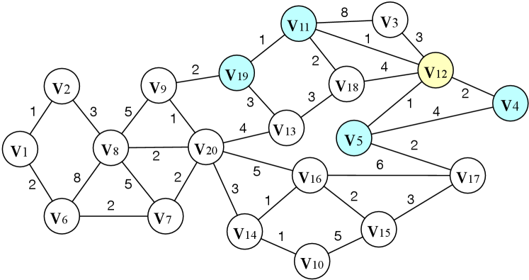
Problem Definition. Given a road network $G=(V,E)$ , a query vertex $u$ , an integer $k$ , and a set of candidate objects $\mathcal{M}$ $(|\mathcal{M}|>k),\mathcal{M}\subseteq V(G)$ ), we aim to computes $k$ objects from $\mathcal{M}$ , denoted by ${\mathsf{V_{k}}}(u)$ , such that $\forall v\in{\mathsf{V_{k}}}(u),$ $w\in\mathcal{M}\setminus{\mathsf{V_{k}}}(u),$ ${\mathsf{dist}}(u,v)\leq{\mathsf{dist}}(u,w)$ .

Example 2.1.

Consider the graph $G$ in Figure 2 and assume all vertices are in the candidate object set. For a given query vertex $v_{12}$ and $k=5$ , $V_{5}(v_{12})=\{v_{12},v_{5},v_{11},v_{4},v_{19}\}$ . The corresponding distances between $v_{12}$ and vertex in $V_{5}(v_{12})$ are $0,1,1,2$ and $2$ respectively.

3. The State-of-the-art Solution

${\mathsf{TEN}}\textrm{-}{\mathsf{Index\ }}$ (Ouyang et al., 2020a) is the state-of-the-art index-based approach for $k$ NN queries on road networks. ${\mathsf{TEN}}\textrm{-}{\mathsf{Index\ }}$ designs an index based on tree decomposition (Robertson and Seymour, 1984; Xu et al., 2005) and $\mathsf{H2H}$ - $\mathsf{Index}$ (Ouyang et al., 2018), which proves superiority over other existing approaches. Specifically,

Index Structure. ${\mathsf{TEN}}\textrm{-}{\mathsf{Index\ }}$ decomposes the input road network into a tree-like structure by tree decomposition (Xu et al., 2005). Given the decomposed tree structure, each vertex $u$ has a child vertex set $\mathbb{T}(u)$ and an ancestor vertex set $\mathbb{A}(u)$ . Apart from the decomposed tree structure, ${\mathsf{TEN}}\textrm{-}{\mathsf{Index\ }}$ contains the other two parts: $k$ TNN for each vertex $u$ which stores the top $k$ nearest neighbors of $u$ in $\mathbb{T}(u)$ and $\mathsf{H2H}$ - $\mathsf{Index}$ (Ouyang et al., 2018) which is used to compute the shortest distance between $u$ and $v\in\mathbb{A}(u)$ .

Query Processing. Given a query vertex $u$ , for each vertex $v$ in the $k$ NN of $u$ , there exists a vertex $p$ such that $p\in\mathbb{A}(u)\cup\{u\}$ and $v$ in $k$ TNN of $p$ . Following this idea, ${\mathsf{TEN}}\textrm{-}{\mathsf{Index\ }}$ answers the $k$ NN query in $k$ rounds. In each $i$ round ( $1\leq i\leq k$ ), it outputs the top $i$ -th result by iterating the vertices in $\mathbb{A}(u)\cup\{u\}$ and computing the corresponding shortest distance through $\mathsf{H2H}$ - $\mathsf{Index}$ .

Index Construction. To construct the index, ${\mathsf{TEN}}\textrm{-}{\mathsf{Index\ }}$ first decomposes the graph following (Xu et al., 2005). With the decomposed tree, $\mathbb{A}(u)$ and $\mathbb{T}(u)$ can be obtained accordingly. After that, ${\mathsf{TEN}}\textrm{-}{\mathsf{Index\ }}$ builds the $\mathsf{H2H}$ - $\mathsf{Index}$ based on (Ouyang et al., 2018). At last, the $k$ TNN for each vertex is constructed by querying the shortest distance of corresponding vertex pairs through $\mathsf{H2H}$ - $\mathsf{Index}$ .

Drawbacks. Although ${\mathsf{TEN}}\textrm{-}{\mathsf{Index\ }}$ accelerates the $k$ NN query processing on road network, the following drawbacks limit its applicability in practice:

•

Oversized Index. The size of ${\mathsf{TEN}}\textrm{-}{\mathsf{Index\ }}$ is generally huge in practice. As verified in our experiments, the size of ${\mathsf{TEN}}\textrm{-}{\mathsf{Index\ }}$ on $\mathsf{USA}$ (only $23,947,347$ vertices and $58,333,344$ edges) exceeds $172.80$ GB, in which $\mathsf{H2H}$ - $\mathsf{Index}$ takes $169.23$ GB space.
•

Long Query Delay. To answer a $k$ NN query regarding vertex $u$ , ${\mathsf{TEN}}\textrm{-}{\mathsf{Index\ }}$ has to iterate the vertices in $\mathbb{A}(u)\cup\{u\}$ and compute the corresponding shortest distance in $k$ rounds. Moreover, the shortest distance computation is not free, and needs heavy exploration on the $\mathsf{H2H}$ - $\mathsf{Index}$ . These two factors lead to long query delay of $\mathsf{TEN}$ - $\mathsf{Index}$ .
•

Prohibitive Indexing Time. As shown in the above, to construct the index, ${\mathsf{TEN}}\textrm{-}{\mathsf{Index\ }}$ has to decompose the road network first, and then build the $\mathsf{H2H}$ - $\mathsf{Index}$ and compute the $k$ TNN accordingly. Obviously, the time cost of these procedures are expensive, especially the $\mathsf{H2H}$ - $\mathsf{Index}$ construction. For the dataset USA, ${\mathsf{TEN}}\textrm{-}{\mathsf{Index\ }}$ takes $19666$ s to construct the index, in which $\mathsf{H2H}$ - $\mathsf{Index}$ consumes $19632$ s.

4. Our Indexing Approach

According to the above analysis, although the use of $\mathsf{H2H}$ - $\mathsf{Index}$ accelerates the query processing of $\mathsf{TEN}$ - $\mathsf{Index}$ , heavily depending on the $\mathsf{H2H}$ - $\mathsf{Index}$ directly leads to the drawbacks of $\mathsf{TEN}$ - $\mathsf{Index}$ . This raises a natural question: why do we need an index for shortest distance such as $\mathsf{H2H}$ - $\mathsf{Index}$ when addressing $k$ NN problem? Based on the logic of $\mathsf{TEN}$ - $\mathsf{Index}$ , partial $k$ NN (namely $k$ TNN) is maintained for each vertex and $\mathsf{H2H}$ - $\mathsf{Index}$ is used to refine the partial $k$ NN to obtain the final results when processing the query. This motivates us to further ask: Is it necessary to maintain the partial $k$ NN? How about maintaining the $k$ NN for each vertex directly as an index? In this way, the drawbacks regarding index size and query delay can be totally addressed. Following this idea, we propose the following index and query processing algorithm.

4.1. Index Structure and Query Processing

Our index just simply records the $k$ NN for each vertex in the graph, which is formally defined as follows:

Definition 4.1.

( $\mathsf{KNN}$ - $\mathsf{Index}$ ) Given a graph $G$ , an integer $k$ and a set of candidate objects $\mathcal{M}$ $(|\mathcal{M}|>k)$ , for each vertex $v\in G$ , $\mathsf{KNN}$ - $\mathsf{Index}$ records the top- $k$ nearest neighbors of $v$ in $\mathcal{M}$ , namely ${\mathsf{V_{k}}}(u)$ , in the increasing order of their shortest distances from $v$ .

Example 4.2.

Given the graph $G$ in Figure 2, assume the candidate object set is all vertices in $G$ and $k=5$ , the $\mathsf{KNN}$ - $\mathsf{Index}$ of $G$ is shown in Figure 3. Take $v_{8}$ as an example, $V_{5}(v_{8})=\{v_{8},v_{20},v_{2},v_{9},v_{1}\}$ , with shortest distance 0, 3, 3, 4 and 4 respectively.

$v$	$\mathsf{KNN}$ - $\mathsf{Index}$	$v$	$\mathsf{KNN}$ - $\mathsf{Index}$
$v_{1}$	$(v_{1},0)(v_{2},1)(v_{6},2)(v_{7},4)(v_{8},4)$	$v_{11}$	$(v_{11},0)(v_{12},1)(v_{19},1)(v_{5},2)(v_{18},2)$
$v_{2}$	$(v_{2},0)(v_{1},1)(v_{6},3)(v_{8},3)(v_{7},5)$	$v_{12}$	$(v_{12},0)(v_{11},1)(v_{5},1)(v_{4},2)(v_{19},2)$
$v_{3}$	$(v_{3},0)(v_{12},3)(v_{5},4)(v_{11},4)(v_{4},5)$	$v_{13}$	$(v_{13},0)(v_{18},3)(v_{19},3)(v_{11},4)(v_{20},4)$
$v_{4}$	$(v_{4},0)(v_{12},2)(v_{5},3)(v_{11},3)(v_{19},4)$	$v_{14}$	$(v_{14},0)(v_{10},1)(v_{16},1)(v_{15},3)(v_{20},3)$
$v_{5}$	$(v_{5},0)(v_{12},1)(v_{11},2)(v_{17},2)(v_{4},3)$	$v_{15}$	$(v_{15},0)(v_{16},2)(v_{14},3)(v_{17},3)(v_{10},4)$
$v_{6}$	$(v_{6},0)(v_{1},2)(v_{7},2)(v_{2},3)(v_{20},4)$	$v_{16}$	$(v_{16},0)(v_{14},1)(v_{10},2)(v_{15},2)(v_{20},4)$
$v_{7}$	$(v_{7},0)(v_{6},2)(v_{20},2)(v_{9},3)(v_{1},4)$	$v_{17}$	$(v_{17},0)(v_{5},2)(v_{12},3)(v_{15},3)(v_{11},4)$
$v_{8}$	$(v_{8},0)(v_{20},2)(v_{2},3)(v_{9},3)(v_{1},4)$	$v_{18}$	$(v_{18},0)(v_{11},2)(v_{12},3)(v_{13},3)(v_{19},3)$
$v_{9}$	$(v_{9},0)(v_{20},1)(v_{19},2)(v_{7},3)(v_{8},3)$	$v_{19}$	$(v_{19},0)(v_{11},1)(v_{9},2)(v_{12},2)(v_{5},3)$
$v_{10}$	$(v_{10},0)(v_{14},1)(v_{16},2)(v_{15},4)(v_{20},4)$	$v_{20}$	$(v_{20},0)(v_{9},1)(v_{7},2)(v_{8},2)(v_{14},3)$

Figure 3.

\mathsf{KNN}

\mathsf{Index}

G

(

k=5

)

Query Processing. Based on our $\mathsf{KNN}$ - $\mathsf{Index}$ , for a $k$ NN query regarding a vertex $v$ , we can answer the query directly by retrieving the corresponding items of $v$ in the $\mathsf{KNN}$ - $\mathsf{Index}$ .

4.2. Theoretical Analysis

Following the index structure and query processing algorithm, we have the following theoretical results.

Optimal Query Processing. Since our query processing algorithm can answer the query directly by scanning the corresponding items of the query vertex in the $\mathsf{KNN}$ - $\mathsf{Index}$ , the following theorem exists obviously:

Theorem 4.3.

Given a $k$ NN query, our algorithm takes $O(k)$ time to process the query.

To answer a $k$ NN query, any algorithm needs to output the $k$ results at least, which takes $O(k)$ time. On the other hand, Theorem 4.3 shows the time complexity of our query processing algorithm is $O(k)$ . Therefore, the optimality holds.

Incremental Polynomial Query Processing. Consider an algorithm that returns several results. Let $k$ be the number of results in the output. An algorithm is said to have incremental polynomial if for all $i\leq k$ , the output time of the first $i$ results is bounded by a polynomial function of the input size and $i$ (Chang et al., 1994). Since the items for each vertex $v$ in the $\mathsf{KNN}$ - $\mathsf{Index}$ are recorded in the increasing order of their distance from $v$ , we have:

Theorem 4.4.

Given a $k$ NN query regarding $v$ , for every $1\leq i\leq k$ , our algorithm outputs the top $i$ -th nearest neighbor in $O(i)$ time.

Theorem 4.4 shows that our query processing algorithm is incremental polynomial, indicating that it progressively provides results for a query within a bounded delay. The capability of incremental polynomial query processing is considered as a significant technical contribution of ${\mathsf{TEN}}\textrm{-}{\mathsf{Index\ }}$ (Ouyang et al., 2020a) and Theorem 4.4 confirms that our algorithm also possesses this desirable theoretical guarantee.

Bounded Index Space. Since $\mathsf{KNN}$ - $\mathsf{Index}$ only stores the top- $k$ nearest neighbors of each vertex in the road network, we have:

Theorem 4.5.

Given a road network $G$ and an integer $k$ , the size of $\mathsf{KNN}$ - $\mathsf{Index}$ is bounded by $O(n\cdot k)$ .

Remark. According to the above analysis, $\mathsf{KNN}$ - $\mathsf{Index}$ processes a query in optimal time while ${\mathsf{TEN}}\textrm{-}{\mathsf{Index\ }}$ takes $O(h\cdot k)$ time ( $h$ is the height of the tree decomposition), which means $\mathsf{KNN}$ - $\mathsf{Index}$ surpasses ${\mathsf{TEN}}\textrm{-}{\mathsf{Index\ }}$ at the query processing. For the index size, the size of $\mathsf{KNN}$ - $\mathsf{Index}$ is $O(n\cdot k)$ while that of ${\mathsf{TEN}}\textrm{-}{\mathsf{Index\ }}$ is $O(n\cdot h)$ . As introduced in Section 1, the $k$ value of $k$ NN search in real road network applications is not large, therefore, the index size of $\mathsf{KNN}$ - $\mathsf{Index}$ is advantageous compared with ${\mathsf{TEN}}\textrm{-}{\mathsf{Index\ }}$ in practice. Note that although (Ouyang et al., 2020a) claims TEN-Index is parameter-free index, both TEN-Index and KNN-Index constructs their index based on a specific $k$ , which means we needs to construct different indices for different values of $k$ . A compromise solution to address this problem for ${\mathsf{TEN}}\textrm{-}{\mathsf{Index\ }}$ and our index is that we can construct the index based on a moderately large $k$ value, and the $k$ NN search with smaller $k$ values can be answered based on the constructed index directly.

5. Index Construction

Based on the structure of $\mathsf{KNN}$ - $\mathsf{Index}$ , it can be constructed straightforwardly by computing the top $k$ nearest neighbors of each vertex through $\mathsf{Dijkstra^{\prime}s}$ algorithm or $\mathsf{TEN}$ - $\mathsf{Index}$ . However, these approaches are time-consuming and inefficient to handle large road network. In this section, we present our new approach to construct the $\mathsf{KNN}$ - $\mathsf{Index}$ .

5.1. Key Properties of ${\mathsf{V_{k}}}(u)$

The above discussed direct approaches using $\mathsf{Dijkstra^{\prime}s}$ algorithm or ${\mathsf{TEN}}\textrm{-}{\mathsf{Index\ }}$ compute the $k$ nearest neighbors for each vertex independently, which misses the potential opportunities to re-use the intermediate results during the index construction. In this section, we introduce two important properties regarding the distance computation, which lays the foundation for our computation-sharing index construction algorithms. We first define:

Definition 5.1.

(Bridge Neighbor Set) Given a vertex $u\in V(G)$ , the bridge neighbor set of $u$ , denoted by ${\mathsf{BNS}}(u)$ , is the set of $u^{\prime}s$ neighbors $v$ such that the weight of the edge $(u,v)$ is equal to the distance between $u$ and $v$ in $G$ , i.e., ${\mathsf{BNS}}(u)=\{v|v\in{\mathsf{nbr}}(u,G)\wedge\phi((u,v),G)={\mathsf{dist}}((u,v),G)\}$ .

Example 5.2.

Consider $v_{8}$ in Figure 2. ${\mathsf{nbr}}(v_{8},G)=\{v_{2},v_{6},v_{7},v_{20},\\ v_{9}\}$ . The shortest path between $v_{8}$ and $v_{9}$ is $(v_{8},v_{20},v_{9})$ , and the distance is ${\mathsf{dist}}((v_{8},v_{9}),G)=3$ . As ${\mathsf{dist}}((v_{8},v_{9}),G)\neq\phi((v_{8},v_{9}),G)$ , $v_{9}$ is not in ${\mathsf{BNS}}(v_{8})$ . Similarly, $v_{6}$ and $v_{7}$ also does not belong to ${\mathsf{BNS}}(v_{8})$ . For the graph $G$ in Figure 2, the bridge neighbor set of $v_{8}$ is ${\mathsf{BNS}}(v_{8})=\{v_{2},v_{20}\}$ .

Based on Definition 5.1, we have following property regarding the bridge neighbor set of $u$ and its $k$ nearest neighbors:

Property 1.

Given a vertex $u\in V(G)$ , ${\mathsf{V_{k}}}(u)\subseteq\cup_{v\in{\mathsf{BNS}}(u)}{\mathsf{V_{k}}}(v)$ .

Proof: We prove this property by contradiction. Assume that $w\in{\mathsf{V_{k}}}(u)$ but $w\notin\cup_{v\in{\mathsf{BNS}}(u)}{\mathsf{V_{k}}}(v)$ . According to Definition 5.1, the shortest path between $w$ and $u$ must pass through one vertex $v\in{\mathsf{BNS}}(u)$ such that for all $v_{i}\in{\mathsf{V_{k}}}(v)$ , $i\in[1,k]$ , we have ${\mathsf{dist}}(v,v_{i})<{\mathsf{dist}}(w,v)$ . Therefore, ${\mathsf{dist}}(u,v)+{\mathsf{dist}}(v,v_{i})<{\mathsf{dist}}(u,v)+{\mathsf{dist}}(v,w)$ . This implies that there are at least $k$ vertices whose distance to $u$ are smaller than the distance between $u$ and $w$ , which contradicts $w\in{\mathsf{V_{k}}}(u)$ . The proof completes. $\Box$

Following Property 1, we have:

Property 2.

Given a vertex $u\in V(G)$ , ${\mathsf{dist}}((u,w),G)={\mathsf{min}}_{v\in{\mathsf{BNS}}(u)}\\ \{{\mathsf{dist}}((u,v),G)+{\mathsf{dist}}((v,w),G)\}$ where $w\in{\mathsf{V_{k}}}(u)$ .

Proof: According to Definition 5.1, for $\forall w\in{\mathsf{V_{k}}}(u)$ , each shortest path between $w$ and $u$ must pass through at least one vertex $v\in{\mathsf{BNS}}(u)$ , so we have ${\mathsf{dist}}(u,w)={\mathsf{dist}}(u,v)+{\mathsf{dist}}(v,w)$ . $\Box$

Based on Property 1, when a vertex $w\in{\mathsf{V_{k}}}(u)$ , $w$ must be in $\cup_{v\in{\mathsf{BNS}}(u)}{\mathsf{V_{k}}}(v)$ . Moreover, when the bridge neighbor set ${\mathsf{BNS}}(u)$ of $u$ , the distance ${\mathsf{dist}}(u,v)$ and ${\mathsf{V_{k}}}(v)$ ( ${\mathsf{dist}}((v,w),G)$ accordingly where $w\in{\mathsf{V_{k}}}(v)$ ) for all $v\in{\mathsf{BNS}}(u)$ have been computed, we can compute ${\mathsf{dist}}((u,w),G)$ for each $w\in\cup_{v\in{\mathsf{BNS}}(u)}{\mathsf{V_{k}}}(v)$ efficiently following Property 2. Obviously, ${\mathsf{V_{k}}}(u)$ just selects $k$ vertices from $\cup_{v\in{\mathsf{BNS}}(u)}{\mathsf{V_{k}}}(v)$ with the smallest distance values. Therefore, if we process the vertices in $G$ in a certain order, and when processing each vertex $u$ , the vertices $v\in{\mathsf{BNS}}(u)$ and ${\mathsf{V_{k}}}(v)$ have been computed, then ${\mathsf{V_{k}}}(u)$ and thereby $\mathsf{KNN}$ - $\mathsf{Index}$ can be computed efficiently by sharing the computed results. The remaining problem is how to make this idea practically applicable. In next section, we present a bottom-up computation-sharing algorithm, which paves the way to our final index construction algorithm.

5.2. A Bottom-Up Computation-Sharing Algorithm

To compute the bridge neighbor set and share the computation effectively, we construct the index based on the bridge neighbor preserved graph $G^{\prime}$ of the road network $G$ , which is defined as:

Definition 5.3.

(BN-Graph) Given a road network $G$ , a graph $G^{\prime}$ is a bridge neighbor preserved graph ( $\mathsf{BN}$ - $\mathsf{Graph}$ ) of $G$ if (1) $V(G^{\prime})=V(G)$ ; (2) for each edge $(u,v)\in E(G^{\prime})$ , $\phi((u,v),G^{\prime})={\mathsf{dist}}((u,v),G)$ ; (3) for any two vertices $u,v\in V(G^{\prime})$ , ${\mathsf{dist}}((u,v),G^{\prime})={\mathsf{dist}}((u,v),G)$ .

G^{\prime}\leftarrow G

;

2 for each $w\in V(G)$ in increasing order of $\pi(w)$ do

\mathcal{N}\leftarrow\{v|v\in{\mathsf{nbr}}(w,G^{\prime})\wedge\pi(v)>\pi(w)\}

;

4 for each pair of vertices $u,v\in\mathcal{N}$ do

5 if $(u,v)\notin E(G^{\prime})$ then

6 insert

(u,v)

into

G^{\prime}

;

\phi((u,v),G^{\prime})\leftarrow\phi((u,w),G^{\prime})+\phi((w,v),G^{\prime})

;

9 else if $\phi((u,w),G^{\prime})+\phi((w,v),G^{\prime})<\phi((u,v),G^{\prime})$ then

\phi((u,v),G^{\prime})\leftarrow\phi((u,w),G^{\prime})+\phi((w,v),G^{\prime})

;

12for each $w\in V(G)$ in decreasing order of $\pi(w)$ do

\mathcal{N}\leftarrow\{v|v\in{\mathsf{nbr}}(w,G^{\prime})\wedge\pi(v)>\pi(w)\}

;

14 for each pair of $u,v\in\mathcal{N}$ do

15 if $\phi((w,v),G^{\prime})+\phi((v,u),G^{\prime})<\phi((w,u),G^{\prime})$ then

\phi((w,u),G^{\prime})\leftarrow\phi((w,v),G^{\prime})+\phi((v,u),G^{\prime})

;

17 mark

(w,u)

as removed;

19remove all the marked edges in

G^{\prime}

;

20 for each $v\in V(G^{\prime})$ do

{\mathsf{BNS}}(v)\leftarrow{\mathsf{nbr}}(v,G^{\prime})

;

Algorithm 1

{\mathsf{SD}}\textrm{-}{\mathsf{Graph}}\textrm{-}{\mathsf{Gen}}(G,\pi)

Based on Definition 5.3, we propose Algorithm 1 to compute the $\mathsf{BN}$ - $\mathsf{Graph}$ of an input road network and obtain the bridge neighbor set for each vertex accordingly. Intuitively, a $\mathsf{BN}$ - $\mathsf{Graph}$ of $G$ with larger bridge neighbor set for each vertex has more potential possibility to share the computation following the analysis of Section 5.1. Meanwhile, the construction of $\mathsf{BN}$ - $\mathsf{Graph}$ should not be costly. Following this idea, for a given road network $G$ and a total vertex order $\pi$ (the order used in our paper is discussed at the end of this section), our algorithm (Algorithm 1) contains two steps to construct $\mathsf{BN}$ - $\mathsf{Graph}$ : (1) Edge insertion, it aims to add edges to connect vertices to enlarge the bridge neighbor set. (2) Edge deletion, it deletes edges to guarantee that the bridge neighbor set is enlarged correctly. Specifically,

$\bullet$ Step 1. Edge Insertion: Given a graph $G$ and a rank over all vertices in $G$ , it initializes $G^{\prime}$ as $G$ , and iterates every vertex in the increasing order of $\pi(w)$ (line 1-2). For every pair of vertices $u,v$ among the neighbors of $w$ in $G^{\prime}$ with higher ranks than $w$ , if $(u,v)\notin E(G^{\prime})$ , a new edge $(u,v)$ with weight $\phi((u,v),G^{\prime})=\phi((u,w),G^{\prime})+\phi((v,w),G^{\prime})$ is inserted into $G^{\prime}$ (line 5-7). Otherwise, if $\phi((u,w),G^{\prime})+\phi((w,v),G^{\prime})<\phi((u,v),G^{\prime})$ , it updates $\phi((u,v),G^{\prime})$ as $\phi((u,w),G^{\prime})$ $+\phi((w,v),G^{\prime})$ (line 8-9).

$\bullet$ Step 2. Edge Deletion: After the edge insertion step, it further iterates the vertex in the decreasing order of $\pi(w)$ (line 10). For every pair of vertices $u,v$ among the neighbors of $w$ in $G^{\prime}$ with higher ranks than $w$ (line 11-12), if $\phi((w,v),G^{\prime})+\phi((v,u),G^{\prime})<\phi((w,u),G^{\prime})$ , it updates $\phi((w,u),G^{\prime})$ as $\phi((w,v),G^{\prime})+\phi((v,u),G^{\prime})$ and marks the updated edge as removed (line 13-15). At last, the marked edges in $G^{\prime}$ are removed (line 16), and ${\mathsf{BNS}}(w)$ for each vertex is set as ${\mathsf{nbr}}(w,G^{\prime})$ (line 17-18).

Example 5.4.

Consider the road network $G$ in Figure 2 and assume the vertex order $\pi=(v_{1},v_{2},...,v_{20})$ , the $\mathsf{BN}$ - $\mathsf{Graph}$ $G^{\prime}$ of $G$ is shown in Figure 4. To construct $G^{\prime}$ , we first conduct the edge insertion step. For $v_{1}$ , its $\mathcal{N}$ is $\{v_{2},v_{6}\}$ . There exists no edge $(v_{2},v_{6})$ in $G^{\prime}$ currently, then $(v_{2},v_{6})$ with $\phi((v_{2},v_{6}),G^{\prime})=3$ is added into $G^{\prime}$ . The procedure continues until all vertices are processed. In the edge deletion step, vertices are processed in the reverse order of $\pi$ . Take $v_{7}$ as an example. When processing $v_{7}$ , its $\mathcal{N}$ is $\{v_{8},v_{20}\}$ . Since $\phi((v_{7},v_{20}),G^{\prime})+\phi((v_{20},v_{8}),G^{\prime})=2+2<\phi((v_{7},v_{8}),G^{\prime})=5$ , $(v_{7},v_{8})$ is marked. When all the vertices are processed, the marked edges are removed, and Figure 4 shows the final $G^{\prime}$ .

Based on the procedure of Algorithm 1, we have:

Lemma 5.5.

The graph $G^{\prime}$ generated at the end of Algorithm 1 is a $\mathsf{BN}$ - $\mathsf{Graph}$ of $G$ .

Proof: Based on Algorithm 1, it is direct that $V(G^{\prime})=V(G)$ , meeting the condition (1) of $\mathsf{BN}$ - $\mathsf{Graph}$ . For any two vertices $u,v\in G$ , ${\mathsf{dist}}((u,v),G)=\sum_{i=1}^{n}\phi((v_{i-1},v_{i}),G)$ , where $\phi((v_{i-1},v_{i}),G)={\mathsf{dist}}((v_{i-1},v_{i}),G)$ . Clearly, $G^{\prime}$ retains all edges with $\phi((u,v),G)={\mathsf{dist}}((u,v),G)$ in $G$ and includes all inserted edges with $\phi((u,v),G^{\prime})={\mathsf{dist}}((u,v),G)$ in $G^{\prime}$ . Therefore, for any two vertices $u,v\in G^{\prime}$ , ${\mathsf{dist}}((u,v),G^{\prime})={\mathsf{dist}}((u,v),G)$ , satisfying the condition (3) of $\mathsf{BN}$ - $\mathsf{Graph}$ . Next, we prove that $G^{\prime}$ satisfies condition (2) via induction. Obviously, for $v_{n-1}$ , $\phi((v_{n-1},v_{n}),G^{\prime})={\mathsf{dist}}((v_{n-1},v_{n}),G)$ . Assume that for $v_{n-k}$ , $\phi((v_{n-k},v),G^{\prime})={\mathsf{dist}}((v_{n-k},v),G)$ for $\forall v\in\mathcal{N}(v_{n-k})$ , $\mathcal{N}(v_{n-k})=\{v|v\in{\mathsf{nbr}}(v_{n-k},G^{\prime})\wedge\pi(v)>\pi(v_{n-k-1})\}$ . Now, we prove it for $v_{n-k-1}$ . Suppose $v_{n-k}$ connects to $v_{n-k-1}$ . From the insertion step, $v_{n-k-1}$ and $\mathcal{N}(v_{n-k-1})$ form a clique. Thus, the shortest path from $v_{n-k-1}$ to $v$ either only contains $v_{n-k-1}$ and $v$ , or passes a vertex in $\mathcal{N}(v_{n-k-1})\setminus\{v_{n-k-1},v\}$ , i.e, ${\mathsf{dist}}((v_{n-k-1},v),G^{\prime})=\phi((v_{n-k-1},v),G^{\prime})$ or ${\mathsf{dist}}((v_{n-k-1},v),G^{\prime})=\min_{u\in\mathcal{N}}(\phi((v_{n-k-1},u),G^{\prime})+{\mathsf{dist}}((u,v),G^{\prime}))$ . Since the $\mathcal{N}(v_{n-k-1})$ includes $v_{k}$ and $\mathcal{N}(v_{k})$ , we have $\phi((u,v),G^{\prime})={\mathsf{dist}}((u,v),G^{\prime})$ for any two vertices $u,v\in\mathcal{N}(v_{n-k-1})$ . Thus, ${\mathsf{dist}}((v_{n-k-1},v),G^{\prime})=\min_{u\in\mathcal{N}(v_{n-k-1})}(\phi((v_{n-k-1},u),G^{\prime})+\phi((u,v),G^{\prime}))$ . As line 10-15 of Algorithm 1 can guarantee that $\phi((u,v),G^{\prime})={\mathsf{dist}}((u,v),G^{\prime})$ , and $G^{\prime}$ satisfies condition (3) of $\mathsf{BN}$ - $\mathsf{Graph}$ , i.e. ${\mathsf{dist}}((u,v),G^{\prime})={\mathsf{dist}}((u,v),G)$ , we have $\phi((u,v),G^{\prime})={\mathsf{dist}}((u,v),G)$ . Therefore, $G^{\prime}$ is a $\mathsf{BN}$ - $\mathsf{Graph}$ of $G$ . $\Box$

Following Lemma 5.5, it is clear that for each vertex $v\in V(G)$ , its $k$ NN in $G$ is the same as that in $G^{\prime}$ based on the condition (3) of Definition 5.3. Moreover, ${\mathsf{nbr}}(w,G^{\prime})$ is the bridge neighbor set of $w$ in $G^{\prime}$ based on the condition (2) of Definition 5.3. The following problem is how to compute ${\mathsf{V_{k}}}(u)$ for each vertex $u$ via $G^{\prime}$ and ${\mathsf{BNS}}(u)$ . According to the discussion in Section 5.1, to fully utilize the intermediate computed results during the $\mathsf{KNN}$ - $\mathsf{Index}$ construction, we define a special type of path based on the given total vertex order as follows:

Definition 5.6.

(Monotonic Rank Path) Given the $\mathsf{BN}$ - $\mathsf{Graph}$ $G^{\prime}$ of a road network $G$ , for a vertex $u\in V(G^{\prime})$ , a path $p(u,v)=(u=v_{1},v_{2},\dots,v_{j}=v)$ in $G^{\prime}$ is a decreasing rank path of $u$ if $\pi(v_{j})<\pi(v_{j-1})<\dots<\pi(v_{1})$ , and it is an increasing rank path of $u$ if $\pi(v_{j})>\pi(v_{j-1})>\dots>\pi(v_{1})$ .

Definition 5.7.

(Monotonic Rank Path Subgraph) Given the $\mathsf{BN}$ - $\mathsf{Graph}$ $G^{\prime}$ of a road network $G$ , for a vertex $u$ , the decreasing rank path subgraph of $u$ , denoted by ${\mathsf{G^{\prime<}}}(u)$ , is the subgraph induced by all decreasing rank paths of $u$ in $G^{\prime}$ . The increasing rank path subgraph, denoted by ${\mathsf{G^{\prime>}}}(u)$ , is the subgraph induced by all increasing rank paths of $u$ in $G^{\prime}$ .

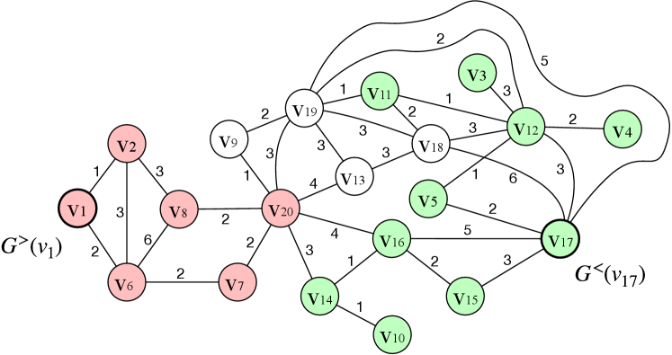
Example 5.8.

Given the $\mathsf{BN}$ - $\mathsf{Graph}$ $G^{\prime}$ in Figure 4, for vertex $v_{1}$ , increasing rank paths of $v_{1}$ contain $p(v_{1},v_{2})=(v_{1},v_{2}),p(v_{1},v_{6})=(v_{1},v_{6}),p(v_{1},v_{8})=(v_{1},v_{2},v_{8})$ or $(v_{1},v_{6},v_{8}),p(v_{1},v_{7})=(v_{1},v_{6},v_{7})$ or $(v_{1},v_{2},v_{6},v_{7}),p(v_{1},v_{20})=(v_{1},v_{2},v_{8},v_{20})$ , $(v_{1},v_{6},v_{8},v_{20})$ , $(v_{1},v_{2},\\ v_{7},v_{20})$ , $(v_{1},v_{2},v_{6},v_{7},v_{20})$ , $(v_{1},v_{2},v_{6},v_{8},v_{20})$ . The increasing rank path subgraph of $v_{1}$ , i.e., ${\mathsf{G^{\prime>}}}(v_{1})$ , is the subgraph induced by these paths, which is shown in pink in Figure 4. The decreasing rank path subgraph of $v_{17}$ , i.e., ${\mathsf{G^{\prime<}}}(v_{17})$ , can be obtained similarly, which is shown in green in Figure 4.

Definition 5.9.

(Decreasing Rank Partial $k$ NN) Given a vertex $u\in V(G)$ and a set of candidate objects $\mathcal{M}$ , the decreasing rank partial $k$ NN of $u$ , denoted by ${\mathsf{V_{k}^{<}}}(u)$ , is the $k$ NN of $u$ in ${\mathsf{G^{\prime<}}}(u)$ .

Lemma 5.10.

Given a vertex $u\in V(G)$ in a road network $G$ , ${\mathsf{V_{k}}}(u)\subseteq\cup_{w\in V({\mathsf{G^{\prime>}}}(u))}{\mathsf{V_{k}^{<}}}(w)$ .

Proof: This lemma can be proved directly based on Property 1. $\Box$

Therefore, if we can obtain ${\mathsf{V_{k}^{<}}}(w)$ for each vertex, we can obtain ${\mathsf{V_{k}}}(u)$ following Lemma 5.10. Moreover, we have:

Lemma 5.11.

Given a road network of $G$ and a set of candidate objects $\mathcal{M}$ , let $u_{1}$ be the vertex with the lowest rank, we have ${\mathsf{V_{k}^{<}}}(u_{1})=\{\mathcal{M}\cap\{u_{1}\}\}$ .

Proof: From Definition 5.7, $V({\mathsf{G^{\prime<}}}(u_{1}))=\{u_{1}\}$ . Based on Definition 5.9, ${\mathsf{V_{k}^{<}}}(u_{1})=\{\mathcal{M}\cap V({\mathsf{G^{\prime<}}}(u_{1}))\}=\{\mathcal{M}\cap\{u_{1}\}\}$ . $\Box$

Based on Lemma 5.11, the decreasing rank partial $k$ NN for the vertex with the lowest rank can be computed directly. Regarding the remaining vertices, we further divide ${\mathsf{BNS}}(u)$ into two parts: ${\mathsf{BNS^{<}}}(u)$ which contains the neighbors of $u$ in $G^{\prime}$ with lower rank than $u$ , i.e., ${\mathsf{BNS^{<}}}(u)=\{v|v\in{\mathsf{BNS}}(u)\wedge\pi(v)<\pi(u)\}$ and ${\mathsf{BNS^{>}}}(u)$ which contains the neighbors of $u$ in $G^{\prime}$ with higher rank than $u$ , i.e., ${\mathsf{BNS^{>}}}(u)=\{v|v\in{\mathsf{BNS}}(u)\wedge\pi(v)>\pi(u)\}$ . We have:

Lemma 5.12.

Given a vertex $u\in V(G)$ in a road network $G$ , ${\mathsf{V_{k}^{<}}}(u)\subseteq\{\mathcal{M}\cap\{u\}\}\cup_{v\in{\mathsf{BNS^{<}}}(u)}{\mathsf{V_{k}^{<}}}(v)$ .

Proof: This lemma can be proved directly based on Property 1 and Definition 5.9. $\Box$

Lemma 5.12 indicates the scope of ${\mathsf{V_{k}^{<}}}(u)$ for each vertex. To obtain ${\mathsf{V_{k}^{<}}}(u)$ , we only need to compute the distance between $u$ and $w\in\{\mathcal{M}\cap\{u\}\}\cup_{v\in{\mathsf{BNS^{<}}}(u)}{\mathsf{V_{k}^{<}}}(v)$ , and retrieve the top $k$ objects. To avoid the expensive $\mathsf{Dijkstra^{\prime}s}$ algorithm, we define:

Definition 5.13.

(Decreasing Rank Shortest Path) Given the $\mathsf{BN}$ - $\mathsf{Graph}$ $G^{\prime}$ of a road network $G$ , for two vertices $u,v\in V(G^{\prime})$ , the decreasing rank shortest path between $u$ and $v$ is the rank decreasing path from $u$ to $v$ with the smallest length in $G^{\prime}$ .

In $\mathsf{BN}$ - $\mathsf{Graph}$ $G^{\prime}$ of $G$ , for any two vertices $u,v\in G^{\prime}$ , one shortest path between $u$ and $v$ is a decreasing rank shortest path. We call the length of decreasing rank shortest path between $u$ and $v$ as decreasing rank distance and denote it as ${\mathsf{dist_{<}}}(u,v)$ . We have:

Lemma 5.14.

Given the $\mathsf{BN}$ - $\mathsf{Graph}$ $G^{\prime}$ of a road network $G$ , for a vertex $u\in V(G^{\prime})$ , ${\mathsf{dist_{<}}}(u,v)={\mathsf{min}}_{w\in{\mathsf{BNS^{<}}}(u)}\{\phi((u,w),G^{\prime})+{\mathsf{dist_{<}}}(w,v)\}$ , where $v\in{\mathsf{V_{k}^{<}}}(u)$ .

Proof: Based on Definition 5.7 and Definition 5.9, we have ${\mathsf{V_{k}^{<}}}(u)\subseteq\{\mathcal{M}\cap V({\mathsf{G^{\prime<}}}(u))\}$ . According to Definition 5.13, for $\forall v\in{\mathsf{G^{\prime<}}}(u)$ , there is one decreasing rank shortest path between $u$ and $v$ , which passes through one vertex $w\in{\mathsf{BNS^{<}}}(u)$ . Therefore, ${\mathsf{dist_{<}}}(u,v)=min_{w\in{\mathsf{BNS^{<}}}(u)}\{\phi((u,w),G^{\prime})+{\mathsf{dist_{<}}}(w,v)\}$ . $\Box$

Lemma 5.15.

Given the $\mathsf{BN}$ - $\mathsf{Graph}$ $G^{\prime}$ of a road network $G$ , for a vertex $u$ , let $v\in{\mathsf{V_{k}^{<}}}(u)\cap{\mathsf{V_{k}}}(u)$ , if ${\mathsf{dist_{<}}}(u,v)={\mathsf{dist}}((u,v),G^{\prime})$ , there is a shortest path between $u$ and $v$ in $G^{\prime}$ , which is also a decreasing rank shortest path.

Proof: According to Definition 5.7 and Definition 5.9, if $v\in{\mathsf{V_{k}^{<}}}(u)$ , we know $v\in V({\mathsf{G^{\prime<}}}(u))$ . Based on Definition 5.13, there is one decreasing rank shortest path between $u$ and $v$ . When ${\mathsf{dist_{<}}}(u,v)\\ ={\mathsf{dist}}((u,v),G^{\prime})$ , there is a shortest path between $u$ and $v$ in $G^{\prime}$ , which is also a decreasing shortest path. $\Box$

Based on Lemma 5.11, Lemma 5.12, and Lemma 5.14, to obtain ${\mathsf{V_{k}^{<}}}(u)$ for each vertex, we can adopt a bottom-up strategy based on the increasing order of $\pi(u)$ , and the computed distance for a lower rank vertex can be re-used to compute the distance for a higher rank vertex. However, ${\mathsf{V_{k}^{<}}}(u)$ only contains the vertices $v\in{\mathsf{V_{k}}}(u)$ whose shortest paths to $u$ pass through ${\mathsf{BNS^{<}}}(u)$ , the vertices $v\in{\mathsf{V_{k}}}(u)$ whose shortest paths to $u$ pass through ${\mathsf{BNS^{>}}}(u)$ does not considered. Unfortunately, these vertices cannot be obtained by only exploring the vertices in $\cup_{v\in{\mathsf{BNS^{>}}}(u)}{\mathsf{V_{k}^{<}}}(v)$ in the similar way as discussed above since this approach only explores the vertices whose ranks are not higher than ${\mathsf{max}}_{v\in{\mathsf{BNS^{>}}}(u)}\pi(v)$ . On the other hand, we have the following lemmas regarding the distance between $u$ and $v\in{\mathsf{V_{k}}}(u)$ based on Lemma 5.10:

Lemma 5.16.

Given the $\mathsf{BN}$ - $\mathsf{Graph}$ $G^{\prime}$ of a road network $G$ , for a vertex $u\in V(G)$ , let $v,v^{\prime}\in V({\mathsf{G^{\prime>}}}(u))$ , ${\mathsf{dist}}((v,v^{\prime}),{\mathsf{G^{\prime>}}}(u))={\mathsf{dist}}((v,v^{\prime}),G)$ .

Proof: This lemma can be proved by Lemma 5.5. $\Box$

Lemma 5.17.

Given the $\mathsf{BN}$ - $\mathsf{Graph}$ $G^{\prime}$ of a road network $G$ , for a vertex $u\in V(G)$ , ${\mathsf{dist}}((u,v),G)={\mathsf{min}}_{w\in V({\mathsf{G^{\prime>}}}(u))}\{{\mathsf{dist}}((u,w),{\mathsf{G^{\prime>}}}\\ (u))+{\mathsf{dist_{<}}}(w,v)\}$ , where $v\in{\mathsf{V_{k}}}(u)$ .

Proof: This lemma can be proved directly based on Lemma 5.10 and Lemma 5.16. $\Box$

G^{\prime}\leftarrow{\mathsf{SD}}\textrm{-}{\mathsf{Graph}}\textrm{-}{\mathsf{Gen}}(G,\pi)

;

\mathcal{S}\leftarrow\emptyset

{\mathsf{V_{k}^{<}}}(\cdot)\leftarrow\emptyset

{\mathsf{V_{k}}}(\cdot)\leftarrow\emptyset

;

3 for each $u$ in increasing order of $\pi(u)$ do

\mathcal{S}\leftarrow\{\mathcal{M}\cap\{u\}\}\cup_{w\in{\mathsf{BNS^{<}}}(u)}{\mathsf{V_{k}^{<}}}(w)

;

5 for each $v\in\mathcal{S}$ do

{\mathsf{dist_{<}}}(u,v)\leftarrow\min_{w\in{\mathsf{BNS^{<}}}(u)}\{\phi((u,w),G^{\prime})+{\mathsf{dist_{<}}}(w,v)\}

;

{\mathsf{V_{k}^{<}}}(u)\leftarrow

k

vertices in

\mathcal{S}

with the smallest

{\mathsf{dist_{<}}}(u,v)

;

9for each $u$ in increasing order of $\pi(u)$ do

10 construct

{\mathsf{G^{\prime>}}}(u)

by conducting

\mathsf{BFS}

search from

u

G^{\prime}

following edge

(v,v^{\prime})

with

\pi(v)<\pi(v^{\prime})

;

11 for each $w\in V({\mathsf{G^{\prime>}}}(u))$ do

12 compute

{\mathsf{dist}}((u,w),{\mathsf{G^{\prime>}}}(u))

;

\mathcal{S}\leftarrow{\mathsf{V_{k}^{<}}}(u)\cup_{w\in V({\mathsf{G^{\prime>}}}(u))}{\mathsf{V_{k}^{<}}}(w)

;

15 for each $v\in\mathcal{S}$ do

{\mathsf{dist}}((u,v),G)\leftarrow\min_{w\in{\mathsf{G^{\prime>}}}(u)}{\mathsf{dist}}((u,w),{\mathsf{G^{\prime>}}}(u))

{\mathsf{dist_{<}}}(w,v)

;

{\mathsf{V_{k}}}(u)\leftarrow

k

vertices in

\mathcal{S}

with the smallest

{\mathsf{dist}}((u,v),G)

;

Algorithm 2

{\mathsf{KNN}}\textrm{-}{\mathsf{Index}}\textrm{-}{\mathsf{Cons}}(G,\pi,\mathcal{M})

Algorithm. By combing the above two cases together, our index construction algorithm is shown in Algorithm 2. It first generates the $\mathsf{BN}$ - $\mathsf{Graph}$ $G^{\prime}$ using Algorithm 1 (line 1). Then, it adopts a bottom-up strategy to compute ${\mathsf{V_{k}^{<}}}(u)$ in the increasing order of $\pi(u)$ (line 2-7). Specifically, for each vertex $u$ , it retrieves $\{\mathcal{M}\cap\{u\}\}\cup_{v\in{\mathsf{BNS^{<}}}(u)}{\mathsf{V_{k}^{<}}}(v)$ based on Lemma 5.12 (line 4) and computes ${\mathsf{dist_{<}}}(u,v)$ based on Lemma 5.14 (line 5-6). Then, ${\mathsf{V_{k}^{<}}}(u)$ is the $k$ vertices in $\mathcal{S}$ with the smallest ${\mathsf{dist_{<}}}(u,v)$ (line 7). After that, it constructs ${\mathsf{G^{\prime>}}}(u)$ by conducting $\mathsf{BFS}$ search from $u$ on $G^{\prime}$ (line 9). And we compute the single source shortest distance ${\mathsf{dist}}((u,w),{\mathsf{G^{\prime>}}}(u))$ from $u$ to each vertex $w$ in ${\mathsf{G^{\prime>}}}(u)$ using the Dijkstra’s Algorithm (line 10-11). Then, following Lemma 5.10, it retrieves $\cup_{w\in V({\mathsf{G^{\prime>}}}(u))}{\mathsf{V_{k}^{<}}}(w)$ (line 12) and computes ${\mathsf{dist}}((u,v),G)$ based on Lemma 5.17 (line 13-14). ${\mathsf{dist_{<}}}(w,v)$ can be obtained from ${\mathsf{V_{k}^{<}}}(w)$ directly. ${\mathsf{dist}}((u,w),{\mathsf{G^{\prime>}}}(u))$ can be computed (line 10-11) after the construction of ${\mathsf{G^{\prime>}}}(u)$ (line $9$ ) following Lemma 5.16. At last, the $k$ vertices in $\mathcal{S}$ with the smallest ${\mathsf{dist}}((u,v),G)$ is returned as ${\mathsf{V_{k}}}(u)$ in line 15.

Example 5.18.

Following the $\mathsf{BN}$ - $\mathsf{Graph}$ $G^{\prime}$ in Figure 4, Figure 5 takes $v_{17}$ as an example to show the procedure of Algorithm 2 to compute ${\mathsf{V}}_{5}(v_{17})$ . According to Algorithm 2, we compute ${\mathsf{V_{5}^{<}}}(v_{17})$ first. Based on $G^{\prime}$ , ${\mathsf{BNS^{<}}}(v_{17})=\{v_{5},v_{12},v_{15},v_{16}\}$ , which is shown in green in Figure 5 (a). Following Algorithm 2, when computing ${\mathsf{V_{5}^{<}}}(v_{17})$ , we already have ${\mathsf{V_{5}^{<}}}(v_{5}),{\mathsf{V_{5}^{<}}}(v_{15}),{\mathsf{V_{5}^{<}}}(v_{12})$ and ${\mathsf{V_{5}^{<}}}(v_{16})$ , which is shown in Figure 5 (b). Consequently, following line 6 of Algorithm 2, we can achieve $\mathcal{S}=\{\mathcal{M}\cap\{v_{17}\}\}\cup_{w\in{\mathsf{BNS^{<}}}(v_{17})}{\mathsf{V_{5}^{<}}}(w)=\{(v_{17},0),(v_{5},2),(v_{12},3),(v_{15},3),(v_{11},4),(v_{4},5),(v_{16},5),(v_{3},6),(v_{14},\\ 6),(v_{10},7)\}$ . Figure 5 (b) shows this set $\mathcal{S}$ for constructing ${\mathsf{V_{5}^{<}}}(v_{17})$ . After sorting distance, we have ${\mathsf{V_{5}^{<}}}(v_{17})=\{(v_{17},0),(v_{5},2),(v_{12},3),\\ (v_{15},3),(v_{11},4)\}$ .

Figure 5 (c) shows the ${\mathsf{G^{\prime>}}}(v_{17})$ in purple with bold lines. Using $\mathsf{Dijkstra^{\prime}s}$ Algorithm, we compute the distance from $v_{17}$ to each vertex in ${\mathsf{G^{\prime>}}}(v_{17})$ . And ${\mathsf{dist}}((v_{17},v_{18}),{\mathsf{G^{\prime>}}}(v_{17}))=6,{\mathsf{dist}}((v_{17},v_{19}),\\ {\mathsf{G^{\prime>}}}(v_{17}))=5,$ and ${\mathsf{dist}}((v_{17},v_{20}),{\mathsf{G^{\prime>}}}(v_{17}))=8$ . Following line 12 of Algorithm 2, when computing ${\mathsf{V_{5}}}(v_{17})$ , we have ${\mathsf{V_{5}^{<}}}(v_{18}),{\mathsf{V_{5}^{<}}}(v_{19})$ and ${\mathsf{V_{5}^{<}}}(v_{20})$ , which is shown in Figure 5 (d). Following line 14 of Algorithm 2, we achieve $\mathcal{S}={\mathsf{V_{5}^{<}}}(v_{17})\cup_{w\in{\mathsf{G^{\prime>}}}(v_{17})}{\mathsf{V_{5}^{<}}}(w)=\{(v_{17},0),(v_{5},2),(v_{12},3),(v_{15},3),(v_{11},4),(v_{19},5),(v_{18},6),(v_{9},7),(v_{20}\\ ,8),(v_{13},9),(v_{7},10),(v_{8},10)\}$ , which is shown in Figure 5 (c). Then, we select $5$ nearest objects from $\mathcal{S}$ as the $\mathsf{KNN}$ - $\mathsf{Index}$ of $v_{17}$ , namely, ${\mathsf{V_{k}}}(v_{17})=\{(v_{17},0),(v_{5},2),(v_{12},3),(v_{15},3),(v_{11},4)\}$ .

The correctness of Algorithm 2 is straightforward following the above discussion. For the efficiency of the algorithm, we have:

Theorem 5.19.

The time complexity of Algorithm 2 is bounded by $O(n\cdot(\rho^{2}+\eta\cdot\tau\cdot log(\eta)+(\tau+\eta)\cdot k))$ , where $\rho$ represents the maximum degree of vertices in the graph generated by Algorithm 1 when Step 1 finishes, $\eta={\mathsf{max}}_{v\in V(G)}|{\mathsf{G^{\prime>}}}(v)|$ and $\tau={\mathsf{max}}_{v\in V(G)}|{\mathsf{BNS^{>}}}(v)|$ .

Proof: Algorithm 1 requires $O(n\cdot\rho^{2})$ time (line 1 of Algorithm 2). Specifically, in the for loop (line 2-9 of Algorithm 1), for each vertex $w$ , line 4-9 of Algorithm 1 takes $O(\rho^{2})$ time and the for loop terminates at $n$ iterations. Therefore, the edge insertion step (line 2-9 of Algorithm 1) requires $O(n\cdot\rho^{2})$ time. Similarly, the edge deletion step requires $O(n\cdot\rho^{2})$ (line 10-16 of Algorithm 1). Scanning all vertices to achieve ${\mathsf{BNS}}(\cdot)$ is bounded by $O(n\cdot\tau)$ (line 17-18 of Algorithm 1). Obviously, for $\forall u\in V(G)$ , $\tau\leq\rho$ . Therefore, the time complexity of Algorithm 1 is $O(n\cdot(\rho^{2}+\tau))=O(n\cdot\rho^{2})$ . In the for loop from line 3 to line 7 of Algorithm 2, line 4 of Algorithm 2 takes $O(\tau\cdot k)$ , since each vertex $u$ is only explored by the vertex $w\in{\mathsf{BNS^{>}}}(u)$ . At the same time with obtaining $\mathcal{S}$ (line 4 of Algorithm 2), line 5-7 of Algorithm 2 could be done. Therefore, ${\mathsf{V_{k}^{<}}}(\cdot)$ construction (line 3-7 of Algorithm 2) requires $O(n\cdot\tau\cdot k)$ time. In the for loop (line 8-15 of Algorithm 2), constructing ${\mathsf{G^{\prime>}}}(u)$ by conducting $\mathsf{BFS}$ search requires $O(\eta\cdot\tau)$ time (line 9 of Algorithm 2). Computing ${\mathsf{dist}}(u,v)$ for $\forall v\in V({\mathsf{G^{\prime>}}}(u))$ via $\mathsf{Dijkstra^{\prime}s}$ algorithm (line 10-11 of Algorithm 2) consumes $O(\eta\cdot\tau\cdot log(\eta))$ time. Obtaining $\mathcal{S}$ and distance computation require $O(\eta\cdot k)$ (line 12-15 of Algorithm 2). Therefore, ${\mathsf{V_{k}}}(\cdot)$ construction (line 8-15 of Algorithm 2) requires $O(n\cdot(\eta\cdot\tau\cdot log(\eta)+(\tau+\eta)\cdot k))$ . In summary, the time complexity of Algorithm 2 is $O(n\cdot(\rho^{2}+\eta\cdot\tau\cdot log(\eta)+(\tau+\eta)\cdot k))$ . $\Box$

Remark. Based on Theorem 5.19, we prefer the generated $\mathsf{BN}$ - $\mathsf{Graph}$ with smaller $\rho$ and $\tau$ . Thus, we use the following heuristic total order $\pi$ in this paper: (1) The vertex with the minimum degree in $G$ has the lowest rank (the vertex with a smallest $\mathsf{id}$ has the lowest rank if more than one vertices have the minimum degree); (2) for two unprocessed vertices $u$ and $v$ in line 2 of Algorithm 1, $\pi(u)>\pi(v)$ if the number of unprocessed neighbors of $u$ is bigger than that of $v$ in $G^{\prime}$ . Note this order can be obtained incidentally in Algorithm 1, and does not affect the time complexity of Algorithm 1.

5.3. A Bidirectional Construction Algorithm

Algorithm 2 adopts a bottom-up strategy to construct the $\mathsf{KNN}$ - $\mathsf{Index}$ with which the computation regarding ${\mathsf{V_{k}^{<}}}(u)$ is well shared. However, it still needs to invoke $\mathsf{Dijkstra^{\prime}s}$ algorithm to compute the distance between $u$ and $w\in V({\mathsf{G^{\prime>}}}(u))$ in line 11-12, which is costly. To address this problem, we propose a new algorithm to further improve the index construction efficiency. Instead of following the sole bottom-up direction which adopted in Algorithm 2, the new algorithm constructs the index in a bidirectional manner, which totally avoids the invocation of $\mathsf{Dijkstra^{\prime}s}$ algorithm. Before introducing our algorithm, we have:

Lemma 5.20.

Given a road network $G$ , let $u_{n}$ be the vertex with the highest rank, ${\mathsf{V_{k}}}(u_{n})={\mathsf{V_{k}^{<}}}(u_{n})$ .

Proof: Following Definition 5.7, $V({\mathsf{G^{\prime>}}}(u_{n}))=\{u_{n}\}$ . Based on Lemma 5.10, ${\mathsf{V_{k}}}(u_{n})\subseteq\cup_{w\in V({\mathsf{G^{\prime>}}}(u_{n}))}{\mathsf{V_{k}^{<}}}(w)={\mathsf{V_{k}^{<}}}(u_{n})$ . $\Box$

Lemma 5.21.

Given the $\mathsf{BN}$ - $\mathsf{Graph}$ $G^{\prime}$ of a road network $G$ , for a vertex $u\in V(G)$ , ${\mathsf{V_{k}}}(u)\subseteq{\mathsf{V_{k}^{<}}}(u)\cup_{w\in{\mathsf{BNS^{>}}}(u)}{\mathsf{V_{k}}}(w)$ .

Proof: This lemma can be proved directly based on Property 1. $\Box$

Lemma 5.20 and Lemma 5.21 imply that if we process the vertices in the decreasing order of their ranks when computing ${\mathsf{V_{k}}}(u)$ , it can re-use the computed information of vertices with higher ranks in the computation of the $k$ NN for vertices with lower ranks. Moreover, we have:

Lemma 5.22.

Given the $\mathsf{BN}$ - $\mathsf{Graph}$ $G^{\prime}$ of a road network $G$ , for a vertex $u\in V(G)$ , ${\mathsf{dist}}((u,v),G)={\mathsf{min}}\{{\mathsf{min}}_{w\in{\mathsf{BNS^{>}}}(u)}\{\phi((u,w),G^{\prime})\\ +{\mathsf{dist}}((w,v),G)\},{\mathsf{dist_{<}}}(u,v)\}$ , where $v\in{\mathsf{V_{k}}}(u)$ .

Proof: For $v\in{\mathsf{V_{k}}}(u)$ , there are two parts. The one part contains all $v$ whose shortest paths to $u$ pass through ${\mathsf{BNS^{>}}}(u)$ , this distance computation can be proved based on Property 2. The other part contains all $v$ whose shortest paths to $u$ pass through ${\mathsf{BNS^{<}}}(u)$ , ${\mathsf{dist_{<}}}(u,v)$ can be directly obtained from ${\mathsf{V_{k}^{<}}}(u)$ based on Lemma 5.15. $\Box$

G^{\prime}\leftarrow{\mathsf{SD}}\textrm{-}{\mathsf{Graph}}\textrm{-}{\mathsf{Gen}}(G,\pi)

;

{\mathsf{V_{k}^{<}}}(\cdot)\leftarrow

line 3-7 of Algorithm 2;

\mathcal{S}\leftarrow\emptyset

{\mathsf{V_{k}}}(\cdot)\leftarrow\emptyset

;

4 for each $u$ in decreasing order of $\pi(u)$ do

\mathcal{S}\leftarrow{\mathsf{V_{k}^{<}}}(u)\cup_{w\in{\mathsf{BNS^{>}}}(u)}{\mathsf{V_{k}}}(w)

;

6 for each $v\in\mathcal{S}$ do

d\leftarrow\min_{w\in{\mathsf{BNS^{>}}}(u)}\{\phi((u,w),G^{\prime})+{\mathsf{dist}}((w,v),G)\};

{\mathsf{dist}}(u,v)\leftarrow\min\{d,{\mathsf{dist_{<}}}(u,v)\}

;

{\mathsf{V_{k}}}(u)\leftarrow

k

vertices in

\mathcal{S}

with the smallest

{\mathsf{dist}}((u,v),G)

;

Algorithm 3

{\mathsf{KNN}}\textrm{-}{\mathsf{Index}}\textrm{-}{\mathsf{Cons}}^{+}(G,\pi,\mathcal{M})

Algorithm. Following Lemma 5.22, our new bidirectional construction algorithm is shown in Algorithm 3. It first generates the $\mathsf{BN}$ - $\mathsf{Graph}$ $G^{\prime}$ of $G$ using Algorithm 1 (line 1) and computes ${\mathsf{V_{k}^{<}}}(u)$ in the same way as Algorithm 2 (line 2). After that, it processes the vertices in the decreasing order of their ranks (line 4-9). For each vertex $u$ , it retrieves ${\mathsf{V_{k}^{<}}}(u)\cup_{w\in{\mathsf{BNS^{>}}}(u)}{\mathsf{V_{k}}}(w)$ based on Lemma 5.21 and stores them in $\mathcal{S}$ (line 5). Then, the distance between $u$ and $v\in\mathcal{S}$ is computed following Lemma 5.22 (line 6-8). Since the index construction procedure follows the decreasing order of $\pi(u)$ , ${\mathsf{V_{k}}}(w)$ for $\forall w\in{\mathsf{BNS^{>}}}(u)$ has been computed before computing ${\mathsf{V_{k}}}(u)$ . ${\mathsf{dist}}((w,v),G)$ can be obtained from ${\mathsf{V_{k}}}(w)$ directly. And $\phi((u,w),G^{\prime})$ can be achieved from $\mathsf{BN}$ - $\mathsf{Graph}$ directly. At last, the $k$ vertices in $\mathcal{S}$ with the smallest ${\mathsf{dist}}((u,v),G)$ is returned as ${\mathsf{V_{k}}}(u)$ in line 9.

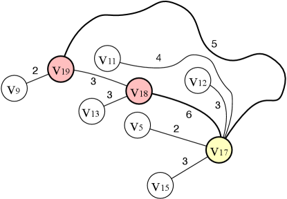
Example 5.23.

Figure 6 shows the ${\mathsf{V_{5}}}(v_{17})$ construction procedure following Algorithm 3. Based on the $\mathsf{BN}$ - $\mathsf{Graph}$ $G^{\prime}$ in Figure 4, for $v_{17}$ , ${\mathsf{BNS^{>}}}(v_{17})=\{v_{18},v_{19}\}$ , which is shown in pink in Figure 6 (a). ${\mathsf{V_{5}^{<}}}(v_{17})$ can be constructed in the same way as shown in Example 5.18. Following line 5 of Algorithm 3, when computing ${\mathsf{V_{5}^{<}}}(v_{17})$ , we already have ${\mathsf{V_{5}^{<}}}(v_{17}),{\mathsf{V_{5}}}(v_{18})$ , and ${\mathsf{V_{5}}}(v_{19})$ , which is shown in Figure 6 (b). According to line 7-8 of Algorithm 3, we have $\mathcal{S}={\mathsf{V_{5}^{<}}}(v_{17})\cup_{w\in{\mathsf{BNS^{>}}}(v_{17})}{\mathsf{V_{5}}}(w)=\{(v_{17},0),(v_{5},2),(v_{12},3),(v_{15},\\ 3),(v_{11},4),(v_{19},5),(v_{18},6),(v_{9},8),(v_{13},9)\}$ . After sorting distance, the $5$ nearest neighbors for $v_{17}$ is selected from the set $\mathcal{S}$ , namely, ${\mathsf{V_{5}}}(v_{17})=\{(v_{17},0),(v_{5},2),(v_{12},3),(v_{15},3),(v_{11},4)\}$ .

Theorem 5.24.

Given a road network $G$ , the time complexity of Algorithm 3 is bounded by $O(n\cdot\rho^{2}+n\cdot\tau\cdot k)$ where $\rho$ represents the maximum degree of vertices in the graph generated by Algorithm 1 when Step 1 finishes, and $\tau={\mathsf{max}}_{v\in V(G)}|{\mathsf{BNS^{>}}}(v)|$ .

Proof: As proved in Theorem 5.19, Algorithm 1 requires $O(n\cdot\rho^{2})$ time (line 1 of Algorithm 3) and ${\mathsf{V_{k}^{<}}}(\cdot)$ construction requires $O(n\cdot\tau\cdot k)$ (line 2 of Algorithm 3). In the for loop from line 4 to line 9 of Algorithm 3, obtaining $\mathcal{S}$ and distance computation require $O(\tau\cdot k)$ (line 5-9 of Algorithm 3) and the loop terminates in $n$ iterations. Therefore, the for loop takes $O(n\cdot\tau\cdot k)$ (line 4-9 of Algorithm 3). In summary, the bidirectional ${\mathsf{KNN}}\textrm{-}{\mathsf{Index}}$ construction (Algorithm 3) requires $O(n\cdot\rho^{2}+n\cdot\tau\cdot k)$ . $\Box$

Compared with Theorem 5.19, Theorem 5.24 shows that the time complexity of our new bidirectional algorithm to construct the index is significantly improved, which is also verified by the experimental results illustrated in Section 7.

6. Candidate Object Update

In some cases, the candidate objects $\mathcal{M}$ may be updated by inserting new objects or deleting existing objects. Straightforwardly, we can reconstruct the index from scratch by Algorithm 3 to handle the update. However, this approach is inefficient as the update of a candidate object may not affect the $k$ NN results of all the vertices. In this section, we discuss how to maintain the $\mathsf{KNN}$ - $\mathsf{Index}$ incrementally when the candidate objects are updated.

Obviously, when a candidate object $u$ is inserted or deleted, the update of $u$ will not affect the $k$ NN results of a vertex $v$ if $u$ and $v$ are far away from each other. Specifically, let $v_{k}$ be the vertex in ${\mathsf{V_{k}}}(v)$ with the largest distance to $v$ . If ${\mathsf{dist}}(u,v)>{\mathsf{dist}}(v,v_{k})$ , then $u$ cannot be in ${\mathsf{V_{k}}}(v)$ , which means deleting or inserting $u$ will not affect ${\mathsf{V_{k}}}(v)$ . Moreover, we have the following lemma based on Property 1 and Property 2:

Lemma 6.1.

Given the $\mathsf{BN}$ - $\mathsf{Graph}$ $G^{\prime}$ of the road network $G$ , for a vertex $v\in V(G))$ , when an object $u$ is inserted/deleted, ${\mathsf{V_{k}}}(v)$ could be affected if and only if there exists at least one vertex $w\in{\mathsf{BNS}}(v)$ whose ${\mathsf{V_{k}}}(w)$ changes due to the update of $u$ .

Proof: This lemma can be directly proved based on Property 1 and Property 2. $\Box$

Therefore, we can maintain the $\mathsf{KNN}$ - $\mathsf{Index}$ starting from the vertex of the updated object $u$ . Based on the definition of $k$ NN, it is clear that ${\mathsf{V_{k}}}(u)$ will be changed. Following Lemma 6.1, the change of ${\mathsf{V_{k}}}(u)$ will possibly lead to the change of ${\mathsf{V_{k}}}(v)$ where $v\in{\mathsf{BNS}}(u)$ . Then, we check whether ${\mathsf{V_{k}}}(v)$ needs to be updated based on ${\mathsf{dist}}(u,v)$ and ${\mathsf{dist}}(v,v_{k})$ as discussed above. We continue to repeat the above procedure recursively, and it is obvious that the $\mathsf{KNN}$ - $\mathsf{Index}$ is correctly maintained when no more vertices whose $k$ NN results change. Based on the above idea, our algorithms to handle the candidate object insertion and deletion are shown in Algorithm 4 and Algorithm 5, respectively.

{\mathsf{dist}}[\cdot]\leftarrow+\infty

;

\mathcal{S}\leftarrow\{\emptyset\}

;

Q\leftarrow\emptyset

;

{\mathsf{dist}}[u]\leftarrow 0

;

\mathcal{S}\leftarrow\{u\}

;

Q.push(u)

;

3 while $Q\neq\emptyset$ do

w\leftarrow Q.{\mathsf{pop}}()

;

5 for each $v\in{\mathsf{BNS}}(w)$ do

{\mathsf{dist}}[v]\leftarrow\min\{{\mathsf{dist}}[v],{\mathsf{dist}}[w]+\phi((w,v),G^{\prime})\}

;

7 if $v\notin\mathcal{S}\wedge{\mathsf{checkIns}}(v,{\mathsf{V_{k}}}(v),{\mathsf{dist}}[v])$ then

Q.{\mathsf{push}}(v)

;

\mathcal{S}\leftarrow\mathcal{S}\cup\{v\}

;

10for each $v\in\mathcal{S}$ do

11 remove

v_{k}

from

{\mathsf{V_{k}}}(v)

; insert

u

into

{\mathsf{V_{k}}}(v)

;

13 Procedure $\mathsf{checkIns}$ $(v,{\mathsf{V_{k}}}(v),d)$

v_{k}\leftarrow

the vertex with the largest distance to

v

{\mathsf{V_{k}}}(v)

;

15 if

{\mathsf{dist}}(v,v_{k})\leq d

then return ${\mathsf{False}}$ ;

16 else return ${\mathsf{True}}$ ;

Algorithm 4

{\mathsf{KNN}}\textrm{-}{\mathsf{Index}}\textrm{-}{\mathsf{Ins}}(G^{\prime},{\mathsf{V_{k}}}(\cdot),u)

Object Insertion. Algorithm 4 shows the algorithm for candidate object insertion. An array ${\mathsf{dist}}[\cdot]$ stores the distance between $u$ and other vertices, a set $\mathcal{S}$ stores vertices whose $k$ NN results should be updated, and a queue $Q$ stores the vertices whose bridge neighbor sets should be checked (line 1). Then, it initializes ${\mathsf{dist}}[u]$ as $0$ and adds $u$ in $\mathcal{S}$ and $Q$ (line 1). After that, it pops a vertex $w$ from $Q$ (line 4), and for each $v\in{\mathsf{BNS}}(w)$ , it computes the distance between $u$ and $v$ , which can be obtained based on the fact ${\mathsf{dist}}(u,v)={\mathsf{min}}_{w^{\prime}\in{\mathsf{BNS}}(v)}\{{\mathsf{dist}}(u,w^{\prime})+{\mathsf{dist}}(w^{\prime},v)\}$ (line 6). Note that instead of visting all $w^{\prime}\in{\mathsf{BNS}}(v)$ , only the vertices whose ${\mathsf{V_{k}}}(w)$ changes due to the update of $u$ need to be explored following Lemma 6.1, which is captured by $Q$ . If $v$ is not in $\mathcal{S}$ and ${\mathsf{dist}}[v]$ is smaller than the distance between $v$ and $v_{k}$ , where $v_{k}$ is the vertex with the largest distance to $v$ in ${\mathsf{V_{k}}}(v)$ which can be obtained directly based on $\mathsf{KNN}$ - $\mathsf{Index}$ , it adds $v$ into $Q$ and $\mathcal{S}$ (line 7-8). The procedure terminates when $Q$ becomes empty (line 3). At last, for each vertex $v\in\mathcal{S}$ , it removes $v_{k}$ from ${\mathsf{V_{k}}}(v)$ and inserts $u$ into ${\mathsf{V_{k}}}(v)$ (line 9-10). When inserting $u$ into ${\mathsf{V_{k}}}(u)$ , ${\mathsf{dist}}[v]$ is the shortest distance between $u$ and $v$ , which can be guaranteed by Lemma 6.1.

Theorem 6.2.

Given the $\mathsf{BN}$ - $\mathsf{Graph}$ $G^{\prime}$ and its corresponding $\mathsf{KNN}$ - $\mathsf{Index}$ of a road network $G$ , Algorithm 4 maintains the $\mathsf{KNN}$ - $\mathsf{Index}$ correctly when an object $u$ is inserted.

Proof: Algorithm 4 (line 5-6) can guarantee ${\mathsf{dist}}[v]$ for $\forall v\in\mathcal{S}$ is the distance between $u$ and $v$ before inserting $u$ to ${\mathsf{V_{k}}}(v)$ for $v\in\mathcal{S}$ (line 9-10). Even though when using ${\mathsf{checkIns}}(v,{\mathsf{V_{k}}}(v),d)$ (line 7), $d$ may not be the distance between $u$ and $v$ and ${\mathsf{checkIns}}(v,{\mathsf{V_{k}}}(v),d)$ returns $\mathsf{True}$ , the final result can not be affected. Since ${\mathsf{dist}}(u,v)\leq d$ , ${\mathsf{checkIns}}$ returning $\mathsf{True}$ denotes that $d<{\mathsf{dist}}(v,v_{k})$ . Therefore, we have ${\mathsf{dist}}(u,v)<{\mathsf{dist}}(v,v_{k})$ . Overall, Algorithm 4 maintains the $\mathsf{KNN}$ - $\mathsf{Index}$ correctly when an object $u$ is inserted. $\Box$

Theorem 6.3.

Given the $\mathsf{BN}$ - $\mathsf{Graph}$ $G^{\prime}$ and its corresponding $\mathsf{KNN}$ - $\mathsf{Index}$ of a road network $G$ , when an object $u$ is inserted, Algorithm 4 maintains the $\mathsf{KNN}$ - $\mathsf{Index}$ in $O(\Delta\cdot\tau^{\prime})$ , where $\Delta=|\mathcal{S}|$ and $\tau^{\prime}={\mathsf{max}}_{v\in V(G)}|{\mathsf{BNS}}(v)|$ .

Proof: The time complexity of ${\mathsf{checkIns}}(v,{\mathsf{V_{k}}}(v),d)$ (line 11-14) is $O(1)$ . In the for loop (line 3-8), for each vertex $w$ , line 5-8 requires $O(\tau^{\prime})$ time and the loop terminates in at most $\Delta$ iterations. Therefore, the for loop (line 3-8) requires $O(\Delta\cdot\tau^{\prime})$ time. In the for loop (line 9-10), removing $v_{k}$ from ${\mathsf{V_{k}}}(v)$ requires $O(1)$ , inserting $u$ into ${\mathsf{V_{k}}}(v)$ in the correct position needs $O(k)$ and the loop stops in $\Delta$ iterations. Therefore, the for loop (line 9-10) requires $O(\Delta\cdot k)$ time. In summary, the overall time complexity of Algorithm 4 is $O(\Delta\cdot(\tau^{\prime}+k)=O(\Delta\cdot\tau^{\prime})$ , since in real applications the parameter $k$ is not large and $k<\tau^{\prime}$ . $\Box$

{\mathsf{dist}}[\cdot]\leftarrow+\infty

;

\mathcal{S}\leftarrow\{\emptyset\}

;

Q\leftarrow\emptyset

;

{\mathsf{dist}}[u]\leftarrow 0

;

\mathcal{S}\leftarrow\{u\}

;

Q.push(u)

;

3 while $Q\neq\emptyset$ do

w\leftarrow Q.{\mathsf{pop}}()

;

5 for each $v\in{\mathsf{BNS}}(w)$ do

{\mathsf{dist}}[v]\leftarrow\min\{{\mathsf{dist}}[v],{\mathsf{dist}}[w]+\phi((w,v),G^{\prime})\}

;

7 if $v\notin\mathcal{S}\wedge{\mathsf{checkDel}}(u,v,{\mathsf{V_{k}}}(v),{\mathsf{dist}}[v])$ then

Q.{\mathsf{push}}(v)

;

\mathcal{S}\leftarrow\mathcal{S}\cup\{v\}

;

10for each $v\in\mathcal{S}$ in decreasing order of $\pi(v)$ do

{\mathsf{processDel}}(v,{\mathsf{BNS}}(v),{\mathsf{V_{k}}}(\cdot))

; delete

u

from

{\mathsf{V_{k}}}(v)

;

13 Procedure $\mathsf{checkDel}$ $(u,v,{\mathsf{V_{k}}}(v),d)$

v_{k}\leftarrow

the vertex with the largest distance to

v

{\mathsf{V_{k}}}(v)

;

15 if

{\mathsf{dist}}(v,v_{k})<d\vee u\notin{\mathsf{V_{k}}}(v)

then return $\mathsf{False}$ ;

17 else return ${\mathsf{True}}$ ;

19Procedure $\mathsf{processDel}$ $(v,{\mathsf{BNS}}(v),{\mathsf{V_{k}}}(\cdot))$

\mathcal{S^{\prime}}\leftarrow\{\cup_{w\in{\mathsf{BNS}}(v)}{\mathsf{V_{k}}}(w)\}\setminus{\mathsf{V_{k}}}(v)

;

v^{\prime}\leftarrow{\mathsf{argmin}}_{v^{\prime}\in\mathcal{S}^{\prime}}{\mathsf{dist}}(v^{\prime},v)

;

23 insert

v^{\prime}

into

{\mathsf{V_{k}}}(v)

;

Algorithm 5

{\mathsf{KNN}}\textrm{-}{\mathsf{Index}}\textrm{-}{\mathsf{Del}}(G^{\prime},{\mathsf{V_{k}}}(\cdot),u)

Object Deletion. Algorithm 5 shows the algorithm for candidate object deletion, which follows a similar framework as Algorithm 4. The main difference is in line 10. When the vertices whose ${\mathsf{V_{k}}}(v)$ need to be updated are determined, Algorithm 5 finds a new vertex $v^{\prime}$ to replace $u$ in ${\mathsf{V_{k}}}(v)$ by procedure $\mathsf{processDel}$ and deletes $u$ from ${\mathsf{V_{k}}}(v)$ . For procedure $\mathsf{processDel}$ , it is easy to know that $v^{\prime}$ must be the vertex in $\{\cup_{w\in{\mathsf{BNS}}(v)}{\mathsf{V_{k}}}(w)\}\setminus{\mathsf{V_{k}}}(v)$ with the smallest distance to $v$ according to Property 1, thus it first retrieves such set of vertices, namely $\mathcal{S^{\prime}}$ (line 16), and finds the vertex in $\mathcal{S^{\prime}}$ with the smallest distance to $v$ (line 17, since the vertices are processed in decreasing order of $\pi(v)$ , ${\mathsf{dist}}(v^{\prime},v)$ can be obtained in the similar way as line 7-8 of Algorithm 3 following the same idea). At last, it inserted $v^{\prime}$ into ${\mathsf{V_{k}}}(v)$ in line 18.

Theorem 6.4.

Given the $\mathsf{BN}$ - $\mathsf{Graph}$ $G^{\prime}$ and its corresponding $\mathsf{KNN}$ - $\mathsf{Index}$ of a road network $G$ , Algorithm 5 maintains the $\mathsf{KNN}$ - $\mathsf{Index}$ correctly when an object $u$ is deleted.

Proof: Algorithm 5 (line 5-6) can guarantee ${\mathsf{dist}}[v]$ for $\forall v\in\mathcal{S}$ is the distance between $u$ and $v$ , before processing each $v\in\mathcal{S}$ (line 9-10). Even though when using ${\mathsf{checkDel}}(v,{\mathsf{V_{k}}}(v),d)$ (line 7), $d$ may not be the distance between $u$ and $v$ and ${\mathsf{checkDel}}(v,{\mathsf{V_{k}}}(v),d)$ returns $\mathsf{True}$ , the final result can not be affected. Since ${\mathsf{dist}}(u,v)\leq d$ , ${\mathsf{checkDel}}$ returning $\mathsf{True}$ denotes that $d<{\mathsf{dist}}(v,v_{k})$ . Therefore, we have ${\mathsf{dist}}(u,v)<{\mathsf{dist}}(v,v_{k})$ . Overall, Algorithm 5 maintains the $\mathsf{KNN}$ - $\mathsf{Index}$ correctly when an object $u$ is deleted. $\Box$

Theorem 6.5.

Given the $\mathsf{BN}$ - $\mathsf{Graph}$ $G^{\prime}$ and its corresponding $\mathsf{KNN}$ - $\mathsf{Index}$ of a road network $G$ , when an object $u$ is deleted, Algorithm 5 maintains the $\mathsf{KNN}$ - $\mathsf{Index}$ in $O(\Delta\cdot\tau^{\prime}\cdot k)$ , where $\Delta=|\mathcal{S}|$ and $\tau^{\prime}={\mathsf{max}}_{v\in V(G)}|{\mathsf{BNS}}(v)|$ .

Proof: The time complexity of ${\mathsf{checkDel}}(u,v,{\mathsf{V_{k}}}(v),d)$ (line 11-14) is $O(1)$ . In the for loop (line 3-8), for each vertex $w$ , line 5-8 requires $O(\tau^{\prime})$ time and the loop terminates in at most $\Delta$ iterations. Therefore, the for loop (line 3-8) requires $O(\Delta\cdot\tau^{\prime})$ time. For the procedure ${\mathsf{processDel}}(v,{\mathsf{BNS}}(v),{\mathsf{V_{k}}}(\cdot)$ (line 15-18), retrieving $\mathcal{S}^{\prime}$ from $\{\cup_{w\in{\mathsf{BNS}}(v)}{\mathsf{V_{k}}}(w)\}\setminus{\mathsf{V_{k}}}(v)$ needs $O(|{\mathsf{BNS}}(v)|\cdot|{\mathsf{V_{k}}}(w)|)=O(\tau^{\prime}\cdot k)$ time (line 16). At the same time with retrieving $\mathcal{S}^{\prime}$ , the vertex $v^{\prime}$ with the smallest distance from $\mathcal{S}^{\prime}$ can be achieved (line 17). Line 18 requires $O(1)$ time, since ${\mathsf{dist}}(v,v^{\prime})\leq{\mathsf{dist}}(v,v_{k})$ and $v^{\prime}$ should be inserted into the end of ${\mathsf{V_{k}}}(v)$ . Therefore, the time complexity of ${\mathsf{processDel}}(v,{\mathsf{BNS}}(v),{\mathsf{V_{k}}}(\cdot)$ (line 15-18) is $O(\tau^{\prime}\cdot k)$ . In the for loop (line 9-10), deleting $u$ from ${\mathsf{V_{k}}}(v)$ requires $O(k)$ , and the loop stops in $\Delta$ iterations. Therefore, the for loop (line 9-10) requires $O(\Delta\cdot\tau^{\prime}\cdot k)$ time. In summary, the overall time complexity of Algorithm 4 is $O(\Delta\cdot\tau^{\prime}\cdot(1+k))=O(\Delta\cdot\tau^{\prime}\cdot k)$ . $\Box$

7. Experiments

In this section, we compare our algorithms with the state-of-the-art method. All experiments are conducted on a machine with an Intel Xeon CPU and 384 GB main memory running Linux.

Dataset	Name	$n$	$m$	$\eta$	$\tau$	$\rho$
New York City	$\mathsf{NY}$	264,346	733,846	725	56	116
San Francisco Bay Area	$\mathsf{BAY}$	321,270	800,172	388	45	100
Colorado	$\mathsf{COL}$	435,666	1,057,066	524	65	122
Florida	$\mathsf{FLA}$	1,070,376	2,712,798	556	49	85
Northwest USA	$\mathsf{NW}$	1,207,945	2,840,208	619	49	119
Northeast USA	$\mathsf{NE}$	1,524,453	3,897,636	1096	81	149
California and Nevada	$\mathsf{CAL}$	1,890,815	4,657,742	795	93	204
Great Lakes	$\mathsf{LKS}$	2,758,119	6,885,658	1674	124	327
Eastern USA	$\mathsf{EUS}$	3,598,623	8,778,114	1089	102	233
Western USA	$\mathsf{WUS}$	6,262,104	15,248,146	1356	128	276
Central USA	$\mathsf{CTR}$	14,081,816	34,292,496	2811	234	531
Full USA	$\mathsf{USA}$	23,947,347	58,333,344	3315	257	587

Table 2. Datasets in Experiments

(a) NY

(b) BAY

(d) FLA

(e) NW

(f) NE

(g) CAL

(h) LKS

(i) EUS

(j) WUS

(k) CTR

(l) USA

Figure 7. Query Processing Time by Varying

k

Datasets. We use twelve publicly available real road networks from DIMACS ²²2http://users.diag.uniroma1.it/challenge9/download.shtml. In each road network, vertices represent intersections between roads, edges correspond to roads or road segments, the weight of an edge is the physical distance between two vertices. Table 2 provides the details about these datasets. Table 2 also shows the value of $\eta$ , $\tau$ and $\rho$ for each road network. Clearly, $\eta$ , $\tau$ and $\rho$ are small in practice.

Algorithms. We compare the following algorithms:

•

$\mathsf{{\mathsf{TEN}}\textrm{-}{\mathsf{Index}}}$ : The state-of-the-art algorithm for $k$ NN queries queries, which is introduced in Section 3.
•

$\mathsf{KNN}$ - $\mathsf{Index}$ : Our proposed algorithms for $k$ NN queries. For the index construction algorithms, we further distinguish between ${\mathsf{KNN}}\textrm{-}{\mathsf{Index}}\textrm{-}{\mathsf{Cons}}$ (Algorithm 2) and ${\mathsf{KNN}}\textrm{-}{\mathsf{Index}}\textrm{-}{\mathsf{Cons}}^{+}$ (Algorithm 3) for comparison.
•

$\mathsf{GLAD}$ : Another algorithm for $k$ NN queries proposed in (Luo et al., 2018), which is introduced in Section 8.
•

$\mathsf{{\mathsf{Dijkstra}}\textrm{-}{\mathsf{Cons}}}$ : Using Dijkstra’s Algorithm to compute top- $k$ nearest neighbors for all vertices in a given graph $G$ to construct the $\mathsf{KNN}$ - $\mathsf{Index}$ as discussed in Section 5.
•

$\mathsf{{\mathsf{TEN}}\textrm{-}{\mathsf{Index}}\textrm{-}{\mathsf{Cons}}}$ : Using $\mathsf{TEN}$ - $\mathsf{Index}$ to compute top- $k$ nearest neighbors for all vertices in a given graph $G$ to construct the $\mathsf{KNN}$ - $\mathsf{Index}$ as discussed in Section 5.

All the algorithms are implemented in C++ and compiled in GCC with -O3. The time cost is measured as the amount of wall-clock time elapsed during the program’s execution. If an algorithm cannot finish in 6 hours, we denote the processing time as $\mathsf{NA}$ .

Parameter Settings. Following previous $k$ NN works (Ouyang et al., 2020a; He et al., 2019; Luo et al., 2018), we randomly select candidate objects in each dataset with a density $\mu=|\mathcal{M}|/|V|$ . The candidate density $\mu$ and the query parameter $k$ settings are shown in Table 3, default values display in bold and italic font.

Parameters	Values
$\mu$	0.5, 0.1, 0.05, 0.01, 0.005, 0.001, 0.0005, 0.0001
$k$	100, 80, 60, 40, 30, 20, 10

Table 3. Parameter Settings

Exp-1: Query Processing Time when Varying $k$ . In this experiment, we evaluate the query processing time of our algorithms $\mathsf{KNN}$ - $\mathsf{Index}$ , the SOTA solutions ${\mathsf{TEN}}\textrm{-}{\mathsf{Index\ }}$ and $\mathsf{GLAD}$ by varying the parameter $k$ . We randomly generate $10,000$ queries and report average running time of each algorithm in Figure 7.

As shown in Figure 7, our algorithm is the most efficient one compared with ${\mathsf{TEN}}\textrm{-}{\mathsf{Index\ }}$ and $\mathsf{GLAD}$ and the growth for query processing time of ${\mathsf{TEN}}\textrm{-}{\mathsf{Index\ }}$ and $\mathsf{GLAD}$ is sharper than that of $\mathsf{KNN}$ - $\mathsf{Index}$ with increase of $k$ . For example, on $\mathsf{NY}$ dataset, when $k$ increases from $10$ to $100$ , the query processing time of ${\mathsf{TEN}}\textrm{-}{\mathsf{Index\ }}$ grows from $13.217$ us to $127.025$ us and $\mathsf{GLAD}$ raises from $18.172$ us to $138.212$ us. However, our $\mathsf{KNN}$ - $\mathsf{Index}$ processing time grows from $0.395$ us to $1.210$ us. This is consistent with our analysis in Section 4.2. For $\mathsf{USA}$ , $\mathsf{GLAD}$ is out of memory, the query processing time for $\mathsf{USA}$ could
not be tested at this and following experiments.

(a) NY

(b) BAY

(d) FLA

(e) NW

(f) NE

(g) CAL

(h) LKS

(i) EUS

(j) WUS

(k) CTR

(l) USA

Figure 8. Query Processing Time by Varying

\mu=|\mathcal{M}|/|V|

Exp-2: Query Processing Time when Varying $\mathcal{M}$ . We also compare our $\mathsf{KNN}$ - $\mathsf{Index}$ with the SOTA solutions ${\mathsf{TEN}}\textrm{-}{\mathsf{Index\ }}$ and $\mathsf{GLAD}$ by varying object $\mathcal{M}$ (the density $\mu=|\mathcal{M}|/|V|$ , therefore, we vary $\mathcal{M}$ by changing $\mu$ ). We randomly generate $10,000$ queries for every dataset. We report the average processing time of each algorithm in Figure 8.

As shown in Figure 8, the query processing time of our algorithm is stable with the decrease of candidate object $\mathcal{M}$ . However, the query processing time of ${\mathsf{TEN}}\textrm{-}{\mathsf{Index\ }}$ and $\mathsf{GLAD}$ increases significantly with the decrease of candidate density $\mu$ . For example, when $\mu=0.0001$ $\mathsf{KNN}$ - $\mathsf{Index}$ achieves 2 orders of magnitude speedup compared with ${\mathsf{TEN}}\textrm{-}{\mathsf{Index\ }}$ in all datasets, and $\mathsf{KNN}$ - $\mathsf{Index}$ achieves 4 orders of magnitude speedup compared with $\mathsf{GLAD}$ . Moreover, the more sparsely the object set distributes, the larger speedup is. This is because our proposed algorithm is optimal regarding query processing as analyzed in Section 4.2.

(a) NY

(b) BAY

(d) FLA

(e) NW

(f) NE

(g) CAL

(h) LKS

(i) EUS

(j) WUS

(k) CTR

(l) USA

Figure 9. Query Processing Time for Different Outputs

Exp-3: Progressive Query Processing. In this experiment, we evaluate the progressive query processing strategy of $\mathsf{KNN}$ - $\mathsf{Index}$ , ${\mathsf{TEN}}\textrm{-}{\mathsf{Index\ }}$ and $\mathsf{GLAD}$ by outputing every $5$ outputs in all datasets with $k=60$ . As shown in Figure 9, the lines of ${\mathsf{TEN}}\textrm{-}{\mathsf{Index\ }}$ and $\mathsf{KNN}$ - $\mathsf{Index}$ are linear in all datasets, and the total time of $\mathsf{KNN}$ - $\mathsf{Index}$ is always smaller than that of $\mathsf{TEN}$ - $\mathsf{Index}$ . The reasons are similar as explained in Exp-1 and Exp-2. $\mathsf{GLAD}$ does not support incremental polynomial query processing, so it has the same the total time for different outputs.

Exp-4: Indexing Time. In this experiment, we evaluate the indexing time for ${\mathsf{KNN}}\textrm{-}{\mathsf{Index}}\textrm{-}{\mathsf{Cons}}^{+}$ , $\mathsf{TEN}$ - $\mathsf{Index}$ , $\mathsf{TEN}$ - $\mathsf{Index}$ - $\mathsf{Cons}$ , $\mathsf{GLAD}$ , ${\mathsf{KNN}}\textrm{-}{\mathsf{Index}}\textrm{-}{\mathsf{Cons}}$ and $\mathsf{Dijkstra}$ - $\mathsf{Cons}$ . Figure 10 shows that ${\mathsf{KNN}}\textrm{-}{\mathsf{Index}}\textrm{-}{\mathsf{Cons}}^{+}$ is the fastest in all datasets, and achieves up to 2 orders of magnitude speedup compared with ${\mathsf{TEN}}\textrm{-}{\mathsf{Index\ }}$ and $\mathsf{GLAD}$ . For example, ${\mathsf{KNN}}\textrm{-}{\mathsf{Index}}\textrm{-}{\mathsf{Cons}}^{+}$ only takes $283.78$ s for $\mathsf{USA}$ while ${\mathsf{TEN}}\textrm{-}{\mathsf{Index\ }}$ costs $19655.68$ s. $\mathsf{TEN}$ - $\mathsf{Index}$ - $\mathsf{Cons}$ and ${\mathsf{TEN}}\textrm{-}{\mathsf{Index\ }}$ takes the similar indexing time as $\mathsf{TEN}$ - $\mathsf{Index}$ - $\mathsf{Cons}$ depends on the $\mathsf{TEN}$ - $\mathsf{Index}$ . They both rely on $\mathsf{H2H}$ - $\mathsf{Index}$ . Also, the indexing time of $\mathsf{GLAD}$ and ${\mathsf{TEN}}\textrm{-}{\mathsf{Index\ }}$ are similar, since $\mathsf{GLAD}$ constructs the additional grid index on the basis of $\mathsf{H2H}$ - $\mathsf{Index}$ . As shown in Figure 10, ${\mathsf{KNN}}\textrm{-}{\mathsf{Index}}\textrm{-}{\mathsf{Cons}}$ cannot complete the index construction within $6$ hours for $\mathsf{CTR}$ and $\mathsf{USA}$ . And for $\mathsf{USA}$ $\mathsf{GLAD}$ is out of memory. $\mathsf{Dijkstra}$ - $\mathsf{Cons}$ cannot finish index construction within $6$ hours for $\mathsf{NE}$ , $\mathsf{LKS}$ , $\mathsf{EUS}$ , $\mathsf{WUS}$ , $\mathsf{CTR}$ and $\mathsf{USA}$ . Although index construction frameworks in ${\mathsf{KNN}}\textrm{-}{\mathsf{Index}}\textrm{-}{\mathsf{Cons}}$ and ${\mathsf{KNN}}\textrm{-}{\mathsf{Index}}\textrm{-}{\mathsf{Cons}}^{+}$ are similar, ${\mathsf{KNN}}\textrm{-}{\mathsf{Index}}\textrm{-}{\mathsf{Cons}}$ consumes much more time compared with ${\mathsf{KNN}}\textrm{-}{\mathsf{Index}}\textrm{-}{\mathsf{Cons}}^{+}$ . For example, for $\mathsf{WUS}$ , ${\mathsf{KNN}}\textrm{-}{\mathsf{Index}}\textrm{-}{\mathsf{Cons}}^{+}$ only costs $50.15$ s, but ${\mathsf{KNN}}\textrm{-}{\mathsf{Index}}\textrm{-}{\mathsf{Cons}}$ costs $42061.20$ s. This is because ${\mathsf{KNN}}\textrm{-}{\mathsf{Index}}\textrm{-}{\mathsf{Cons}}$ first uses BFS to construct ${\mathsf{G^{\prime>}}}(u)$ for each vertex $u\in V(G)$ , and then uses Dijkstra’s Algorithm to compute ${\mathsf{dist}}(u,v)$ for $\forall v\in V({\mathsf{G^{\prime>}}}(u))$ when constructing the index. However, ${\mathsf{KNN}}\textrm{-}{\mathsf{Index}}\textrm{-}{\mathsf{Cons}}^{+}$ adopts a bidirectional construction strategy to avoid the time-consuming BFS search and the computation of Dijkstra’s Algorithm during the index construction. The experimental results demonstrate the efficiency of our proposed algorithm regarding index construction.

Exp-5: Index Size. In this experiment, we evaluate the index size for $\mathsf{KNN}$ - $\mathsf{Index}$ , ${\mathsf{TEN}}\textrm{-}{\mathsf{Index\ }}$ and $\mathsf{GLAD}$ . The experimental results for the $12$ road networks are shown in Figure 11. Figure 11 shows the index size of $\mathsf{KNN}$ - $\mathsf{Index}$ is much smaller than that of ${\mathsf{TEN}}\textrm{-}{\mathsf{Index\ }}$ and $\mathsf{GLAD}$ . For example, for the dataset $\mathsf{USA}$ , the $\mathsf{KNN}$ - $\mathsf{Index}$ size is only $3.57$ GB while ${\mathsf{TEN}}\textrm{-}{\mathsf{Index\ }}$ size is $169.28$ GB, which is $47.42$ times smaller than that of $\mathsf{TEN}$ - $\mathsf{Index}$ .

	USA				CTR
$k$	${\mathsf{TEN}}\textrm{-}{\mathsf{Index\ }}$	$\mathsf{KNN}$ - $\mathsf{Index}$	${\mathsf{TEN}}\textrm{-}{\mathsf{Index\ }}$	$\mathsf{KNN}$ - $\mathsf{Index}$	${\mathsf{TEN}}\textrm{-}{\mathsf{Index\ }}$	$\mathsf{KNN}$ - $\mathsf{Index}$	${\mathsf{TEN}}\textrm{-}{\mathsf{Index\ }}$	$\mathsf{KNN}$ - $\mathsf{Index}$
$k$	Indexing Time (s)	Indexing Time (s)	Index Size (GB)	Index Size (GB)	Indexing Time (s)	Indexing Time (s)	Index Size (GB)	Index Size (GB)
$10$	19669.787	266.005	169.265	1.784	10877.527	169.578	98.021	1.049
$20$	19670.198	283.850	169.277	3.568	10878.179	179.480	98.028	2.908
$30$	19670.336	297.224	169.286	5.353	10881.515	186.859	98.034	3.148
$40$	19671.470	321.845	169.293	7.1369	10882.434	201.225	98.039	4.197
$60$	19672.287	345.169	169.305	10.705	10884.793	215.737	98.046	6.295
$80$	19672.839	382.074	169.315	14.274	10885.981	238.944	98.053	8.393
$100$	19710.726	418.251	169.324	17.842	10887.369	253.219	98.058	10.492

Table 4. Indexing Time and Index Size when Varying

k

Exp-6: Indexing Time and Index Space when Varying $k$ . We evaluate the performance of $\mathsf{KNN}$ - $\mathsf{Index}$ and ${\mathsf{TEN}}\textrm{-}{\mathsf{Index\ }}$ when varying $k$ on $\mathsf{USA}$ and $\mathsf{CTR}$ with $k=10,20,30,40,60,80,100$ . The results on the other datasets are omitted due to similar trends. As shown in Table 4, the index size and the indexing time of ${\mathsf{TEN}}\textrm{-}{\mathsf{Index\ }}$ and $\mathsf{KNN}$ - $\mathsf{Index}$ both increases with the growth of $k$ slightly. For example, when $k$ increases from $10$ to $100$ , the indexing time for $\mathsf{USA}$ increases by $40.940$ s and the index size for $\mathsf{USA}$ increases by $0.059$ GB. This is consistent with our analysis in Section 4.2.

Exp-7: Scalability when Varying Graph Size. In this experiment, we evaluate the scalability of $\mathsf{KNN}$ - $\mathsf{Index}$ , ${\mathsf{TEN}}\textrm{-}{\mathsf{Index\ }}$ and $\mathsf{GLAD}$ . To test the scalability for indexing time and index size, we divide the map of the whole US into $10\times 10$ grids. We select a $1\times 1$ grid in the middle and generate an induced network by all vertices falling the grid. Using this method, we generate $10$ datasets. We report the indexing time and index size for these ten networks in Figure 13. The labels on $x$ -axis represent the number of vertices. For the largest datasets, $\mathsf{GLAD}$ is out of memory. As shown in Figure 13, when the dataset increases from $10^{6}$ to $24*10^{6}$ , the indexing time increases stably for all algorithms, which verifies our $\mathsf{KNN}$ - $\mathsf{Index}$ has a good scalability. Moreover, our $\mathsf{KNN}$ - $\mathsf{Index}$ always outperforms ${\mathsf{TEN}}\textrm{-}{\mathsf{Index\ }}$ and $\mathsf{GLAD}$ . The reasons are similar as explained in Exp-4 and Exp-5.

Exp-8: Object Update. In this experiment, we evaluate the performance of our update algorithms. To generate updated objects, we randomly select an object $u$ with either insertion or deletion. We skip the update if $u\notin\mathcal{M}$ for deletion and $u\in\mathcal{M}$ for insertion. For each dataset, we repeat this step until $10,000$ updates are generated. The average time for each update is reported in Figure 12. The update time of $\mathsf{KNN}$ - $\mathsf{Index}$ is slower than that of ${\mathsf{TEN}}\textrm{-}{\mathsf{Index\ }}$ and that of $\mathsf{GLAD}$ , since our update algorithm needs more time to compute the distance between each vertex and the updated objects. As analyzed in Section 3, ${\mathsf{TEN}}\textrm{-}{\mathsf{Index\ }}$ contains $\mathsf{H2H}$ - $\mathsf{Index}$ , $\mathsf{H2H}$ - $\mathsf{Index}$ can compute the distance between any two vertices efficiently. Therefore, based on $\mathsf{H2H}$ - $\mathsf{Index}$ , ${\mathsf{TEN}}\textrm{-}{\mathsf{Index\ }}$ can finish insertion or deletion in the shorter time. Since $\mathsf{GLAD}$ only needs to update objects’ grid index, the update operation is easier and costs shorter time.

Exp-9: System Throughput. We evaluate the throughput of answering queries mixed by $k$ NN queries and object updates. Following (Ouyang et al., 2020b), the throughput is calculated based on two models, which are (1) Batch Update Arrival + Query First ( $\mathsf{BUA}$ + $\mathsf{QF}$ ) and (2) Random Update Arrival + First Come First Served ( $\mathsf{RUA}$ + $\mathsf{FCFS}$ ) (Luo et al., 2018). We report the throughput of each algorithm under different $k$ and $\mu$ for a representative dataset $\mathsf{NY}$ , which is also used in (Ouyang et al., 2020b). The results are shown in Figure 14. We can see that the throughput of $\mathsf{KNN}$ - $\mathsf{Index}$ is larger for the $\mathsf{BUA}$ + $\mathsf{QF}$ model as our query processing algorithm is very fast. However, in the $\mathsf{RUA}$ + $\mathsf{FCFS}$ model, the throughput of $\mathsf{KNN}$ - $\mathsf{Index}$ is smaller than that of ${\mathsf{TEN}}\textrm{-}{\mathsf{Index\ }}$ and $\mathsf{GLAD}$ . This is because our update algorithm costs more time than the update algorithms for ${\mathsf{TEN}}\textrm{-}{\mathsf{Index\ }}$ and $\mathsf{GLAD}$ . Also, the throughput of $\mathsf{KNN}$ - $\mathsf{Index}$ , ${\mathsf{TEN}}\textrm{-}{\mathsf{Index\ }}$ and $\mathsf{GLAD}$ all will go down with the decrease of $\mu$ . When the candidate density is relatively high, our update algorithms are faster. When $\mu$ decreases in Figure 14(c), our update algorithms cost more time. Even if our query processing time is not affected by $\mu$ , our throughput still decrease with the fall of $\mu$ . For ${\mathsf{TEN}}\textrm{-}{\mathsf{Index\ }}$ and $\mathsf{GLAD}$ , the query processing time and updating time both will be longer with decrease of $\mu$ . Therefore, the throughput of ${\mathsf{TEN}}\textrm{-}{\mathsf{Index\ }}$ and $\mathsf{GLAD}$ have a similar trend with that of $\mathsf{KNN}$ - $\mathsf{Index}$ . In summary, $\mathsf{KNN}$ - $\mathsf{Index}$ is good at handling the $\mathsf{BUA}$ + $\mathsf{QF}$ workload while ${\mathsf{TEN}}\textrm{-}{\mathsf{Index\ }}$ and $\mathsf{GLAD}$ are good at handling $\mathsf{RUA}$ + $\mathsf{FCFS}$ workload, and $\mathsf{KNN}$ - $\mathsf{Index}$ , ${\mathsf{TEN}}\textrm{-}{\mathsf{Index\ }}$ and $\mathsf{GLAD}$ have their respective advantages regarding throughput.

Exp-10: Indexing Time of Different Vertex Total Orders. We evaluate index construction performance using different total orders. We adopt three total orders: (1) degree-based total order in which the vertex with the smallest degree is processed first; (2) id-based total order in which the vertex with the smallest id is processed first; (3) and our proposed total order. As shown in Figure 15, degree-based order can finish $\mathsf{KNN}$ - $\mathsf{Index}$ construction for four small datasets, and id-based order only can construct $\mathsf{KNN}$ - $\mathsf{Index}$ for 3 small datasets within $6$ hours. Our order can finish constructing $\mathsf{KNN}$ - $\mathsf{Index}$ for all datasets, and the construction time in our order is 4 orders of magnitude faster than the other two orders. The experimental results are also consistent with our analysis in Section 5.2.

8. Related Work

The direct approach to answer a $k$ NN query is the $\mathsf{Dijkstra}$ ’s algorithm (Dijkstra, 1959). Nevertheless, this approach is inefficient obviously. Therefore, a plethora of index based $\mathsf{Dijkstra}$ -search enhanced solutions (Papadias et al., 2003b; Demiryurek et al., 2009a; Lee et al., 2010; Zhong et al., 2015; Shen et al., 2017; Luo et al., 2018) are proposed in the literature, which generally adopts the following search framework for a given query vertex $u$ : (1) Initialize the distance for vertices $v$ it connected as their edge weights and other vertices as $+\infty$ . (2) Maintain two vertex sets $S$ and $T$ . $S$ contains vertices whose distance to $u$ is computed. $T$ contains vertices whose distance to $u$ is not computed yet, but have neighbors in $S$ . Initially, $u$ is inserted in $S$ and the neighbors of $u$ are inserted in $T$ . (3) Select one node $v$ with the smallest distance to $u$ from $T$ , and add it to $S$ . Then, the neighbors of $v$ are inserted into $T$ . Here, different indexing methods add different restrictions, pruning unnecessary vertices to be inserted in $T$ , to improve the query processing performance. (4) Repeat (3) until $|S|=k$ .

Specifically, $\mathsf{IER}$ (Papadias et al., 2003b) uses Euclidean distance as a pruning bound to acquire the $k$ NN results. $\mathsf{INE}$ (Papadias et al., 2003b) improves $\mathsf{IER}$ ’s Euclidean distance bound by expending searching space from the query location. (Demiryurek et al., 2009a) adapts a Euclidean restriction-based method to deal with continuous $k$ nearest neighbor problem. (Demiryurek et al., 2009a) divides the map into $N\times N$ grids and records which vertices and edges belong to some grid. Given a query vertex, the fixed distance between grids is used to filter a proximate range. $\mathsf{ROAD}$ (Lee et al., 2010) separates the input graph $G$ into many subgraphs hierarchically and skips the subgraphs without candidate objects to speedup $k$ NN query processing. $\mathsf{G}$ - $\mathsf{tree}$ (Zhong et al., 2015) adapts a binary tree division method to divide a graph into two disjoint subgraphs recursively until the number of vertices in a tree node is smaller than a predefined parameter. In each subgraph, $\mathsf{G}$ - $\mathsf{tree}$ maintains a distance matrix which stores distance between borders and vertices, which is used to prune unnecessary vertex exploration during the $\mathsf{Dijkstra}$ search. $\mathsf{V}$ - $\mathsf{tree}$ (Shen et al., 2017) constructs a similar structure as $\mathsf{G}$ - $\mathsf{tree}$ but adds additional $k$ nearest objects for borders, which leads to a faster query processing than $\mathsf{G}$ - $\mathsf{tree}$ . Based on the contraction hierarchy ( $\mathsf{CH}$ ) (Geisberger et al., 2008), $\mathsf{TOAIN}$ (Luo et al., 2018) constructs a $k$ DNN index recording the top- $k$ nearest neighbors for each vertex $u$ from objects whose ranks are lower than $u$ , where the rank is defined by the contraction hierarchy. To answer a $k$ NN query with vertex $u$ , $\mathsf{TOAIN}$ performs $\mathsf{Dijkstra}$ search from $u$ following the $\mathsf{CH}$ and maintains a candidate result set $R$ . When visiting a vertex $v$ , if there is a vertex $w$ in the $k$ DNN of $v$ such that the distance of $w$ and $u$ is smaller than the $k$ -th distance to $u$ in $R$ , $\mathsf{TOAIN}$ updates $R$ . The processing finishes when the $\mathsf{Dijkstra}$ search is far enough or all vertices are explored. Although the methods design different pruning algorithms to reduce the $\mathsf{Dijkstra}$ search space in step (3), the number of explored vertices cannot be well-bounded. In worst case, these methods degenerate into $\mathsf{Dijkstra}$ ’s algorithm, which leads to long query processing delay unavoidably. For $\mathsf{TOAIN}$ , asit constructs $k$ DNN based on $\mathsf{CH}$ , which causes a relatively huge index size. Additionally, the vertex ranking method in $\mathsf{TOAIN}$ employs $\mathsf{Dijkstra}$ ’s Algorithm, which incurs an expensive time cost regarding index construction. The experimental results of (Ouyang et al., 2020a) also verify above discussions.

Apart from the $\mathsf{Dijkstra}$ -search enhanced solutions, (Li et al., 2018) exploits the massive parallelism of GPU to accelerate the $k$ NN query processing. $\mathsf{GLAD}$ (He et al., 2019) partitions the road network into $2^{x}\times 2^{x}$ girds based on the geographical coordinate of each vertex. When answering a $k$ NN query, it starts the search from the grid containing the query vertex and updates the candidate result via probing vertices in neighbor grids iteratively. It avoids the exploration to the vertices in a grid if the minimum Euclidean distance between any vertex inside the grid and the query vertex is not less than the largest distance in the candidate result. As $\mathsf{GLAD}$ needs to use $\mathsf{H2H}$ - $\mathsf{Index}$ to compute the exact shortest distance to select the final exact $k$ NN results, the query processing is long. Moreover, since $\mathsf{GLAD}$ depends on $\mathsf{H2H}$ - $\mathsf{Index}$ , the index size of $\mathsf{GLAD}$ is huge and the indexing time of $\mathsf{GLAD}$ is long, which are similar to ${\mathsf{TEN}}\textrm{-}{\mathsf{Index\ }}$ (Ouyang et al., 2020a). ${\mathsf{TEN}}\textrm{-}{\mathsf{Index\ }}$ (Ouyang et al., 2020a) is the state-of-the-art approach to $k$ NN query in road network, which has been discussed in Section 3. (Li et al., 2023) extend ${\mathsf{TEN}}\textrm{-}{\mathsf{Index\ }}$ (Ouyang et al., 2020a) and $\mathsf{GLAD}$ (He et al., 2019) onto time-dependent road networks. (Jiang et al., 2023) extends tree decomposition method (Ouyang et al., 2018) to deal with $k$ NN search on flow graph.

Besides, continuous $k$ NN query problem on road network is also studied in the literature (Shahabi et al., 2003; Kolahdouzan and Shahabi, 2005; Cho and Chung, 2005; Mouratidis et al., 2006; Demiryurek et al., 2009b; Cho et al., 2013; Zheng et al., 2016; Kolahdouzan and Shahabi, 2004; Jiang et al., 2023, 2021). Different from our setting, these studies generally assume that the query vertex is moving on the road network, and thus are orthogonal to ours. As a result, the proposed techniques in these studies cannot be used to address our problem.

9. Conclusion

Motivated by existing complex-index-based approaches for classical top $k$ nearest neighbors search in road networks suffers from the long query processing delay, oversized index space, and prohibitive indexing time, we embrace minimalism and design a simple index for $k$ NN query. The index has a well-bounded space and supports progressive and optimal query processing. Moreover, we further design efficient algorithms to support the index construction. Experimental results demonstrate the significant superiority of our index over the state-of-the-art approach.

References

(1)
Abbasifard et al. (2014) Mohammad Reza Abbasifard, Bijan Ghahremani, and Hassan Naderi. 2014. A survey on nearest neighbor search methods. International Journal of Computer Applications 95, 25 (2014).
Airnb ([n.d.]) Airnb. [n.d.]. https://www.airbnb.com/.
Bhatia et al. (2010) Nitin Bhatia et al. 2010. Survey of nearest neighbor techniques. arXiv preprint arXiv:1007.0085 (2010).
Booking ([n.d.]) Booking. [n.d.]. https://www.booking.com/.
Chang et al. (1994) Y. H. Chang, Jia-Shung Wang, and Richard C. T. Lee. 1994. Generating All Maximal Independent Sets on Trees in Lexicographic Order. Inf. Sci. 76, 3-4 (1994), 279–296.
Chernev et al. (2015) Alexander Chernev, Ulf Böckenholt, and Joseph Goodman. 2015. Choice overload: A conceptual review and meta-analysis. Journal of Consumer Psychology 25, 2 (2015), 333–358.
Cho et al. (2013) Hyung-Ju Cho, Se Jin Kwon, and Tae-Sun Chung. 2013. A safe exit algorithm for continuous nearest neighbor monitoring in road networks. Mob. Inf. Syst. 9, 1 (2013), 37–53.
Cho and Chung (2005) Hyung-Ju Cho and Chin-Wan Chung. 2005. An efficient and scalable approach to CNN queries in a road network. In Proceedings of VLDB, Vol. 2. International Conference on VLDB, 865–876.
Demiryurek et al. (2009a) Ugur Demiryurek, Farnoush Banaei-Kashani, and Cyrus Shahabi. 2009a. Efficient continuous nearest neighbor query in spatial networks using euclidean restriction. In Proceedings of SSTD. Springer, 25–43.
Demiryurek et al. (2009b) Ugur Demiryurek, Farnoush Banaei Kashani, and Cyrus Shahabi. 2009b. Efficient Continuous Nearest Neighbor Query in Spatial Networks Using Euclidean Restriction. In Proceedings of SSTD, Vol. 5644. 25–43.
Dianping ([n.d.]) Dianping. [n.d.]. https://www.dianping.com/.
DiDi ([n.d.]) DiDi. [n.d.]. https://www.didiglobal.com.
Dijkstra (1959) Edsger W. Dijkstra. 1959. A note on two problems in connexion with graphs. Vol. 1. 269–271.
Geisberger et al. (2008) Robert Geisberger, Peter Sanders, Dominik Schultes, and Daniel Delling. 2008. Contraction hierarchies: Faster and simpler hierarchical routing in road networks. In Proceedings of WEA. Springer, 319–333.
He et al. (2019) Dan He, Sibo Wang, Xiaofang Zhou, and Reynold Cheng. 2019. An efficient framework for correctness-aware kNN queries on road networks. In Proceedings of ICDE. IEEE, 1298–1309.
Jiang et al. (2023) Wei Jiang, Guanyu Li, Mei Bai, Bo Ning, Xite Wang, and Fangliang Wei. 2023. Graph-Indexed k NN Query Optimization on Road Network. Electronics 12, 21 (2023), 4536.
Jiang et al. (2021) Wei Jiang, Fangliang Wei, Guanyu Li, Mei Bai, Yongqiang Ren, and Jingmin An. 2021. Tree index nearest neighbor search of moving objects along a road network. Wireless Communications and Mobile Computing 2021 (2021), 1–18.
Kolahdouzan and Shahabi (2004) Mohammad R. Kolahdouzan and Cyrus Shahabi. 2004. Voronoi-Based K Nearest Neighbor Search for Spatial Network Databases. In Proceedings of VLDB. 840–851.
Kolahdouzan and Shahabi (2005) Mohammad R. Kolahdouzan and Cyrus Shahabi. 2005. Alternative Solutions for Continuous K Nearest Neighbor Queries in Spatial Network Databases. GeoInformatica 9, 4 (2005), 321–341.
Lee et al. (2010) Ken CK Lee, Wang-Chien Lee, Baihua Zheng, and Yuan Tian. 2010. ROAD: A new spatial object search framework for road networks. IEEE transactions on knowledge and data engineering 24, 3 (2010), 547–560.
Li et al. (2018) Chuanwen Li, Yu Gu, Jianzhong Qi, Jiayuan He, Qingxu Deng, and Ge Yu. 2018. A GPU Accelerated Update Efficient Index for kNN Queries in Road Networks. In Proceedings of ICDE. 881–892.
Li et al. (2023) Jiajia Li, Cancan Ni, Dan He, Lei Li, Xiufeng Xia, and Xiaofang Zhou. 2023. Efficient k NN query for moving objects on time-dependent road networks. The VLDB Journal 32, 3 (2023), 575–594.
Luo et al. (2018) Siqiang Luo, Ben Kao, Guoliang Li, Jiafeng Hu, Reynold Cheng, and Yudian Zheng. 2018. Toain: a throughput optimizing adaptive index for answering dynamic k nn queries on road networks. Proceedings of VLDB 11, 5 (2018), 594–606.
Mouratidis et al. (2006) Kyriakos Mouratidis, Man Lung Yiu, Dimitris Papadias, and Nikos Mamoulis. 2006. Continuous Nearest Neighbor Monitoring in Road Networks. In Proceedings of VLDB. 43–54.
Nodarakis et al. (2017) Nikolaos Nodarakis, Angeliki Rapti, Spyros Sioutas, Athanasios K Tsakalidis, Dimitrios Tsolis, Giannis Tzimas, and Yannis Panagis. 2017. (A) kNN query processing on the cloud: a survey. In Algorithmic Aspects of Cloud Computing: Second International Workshop, ALGOCLOUD 2016, Aarhus, Denmark, August 22, 2016, Revised Selected Papers 2. Springer, 26–40.
OpenRice ([n.d.]) OpenRice. [n.d.]. https://www.openrice.com/.
OpenTable ([n.d.]) OpenTable. [n.d.]. https://www.opentable.com.au/.
Ouyang et al. (2018) Dian Ouyang, Lu Qin, Lijun Chang, Xuemin Lin, Ying Zhang, and Qing Zhu. 2018. When hierarchy meets 2-hop-labeling: Efficient shortest distance queries on road networks. In Proceedings of SIGMOD. 709–724.
Ouyang et al. (2020a) Dian Ouyang, Dong Wen, Lu Qin, Lijun Chang, Ying Zhang, and Xuemin Lin. 2020a. Progressive top-k nearest neighbors search in large road networks. In Proceedings of SIGMOD. 1781–1795.
Ouyang et al. (2020b) Dian Ouyang, Long Yuan, Lu Qin, Lijun Chang, Ying Zhang, and Xuemin Lin. 2020b. Efficient shortest path index maintenance on dynamic road networks with theoretical guarantees. Proceedings of the VLDB Endowment 13, 5 (2020), 602–615.
Papadias et al. (2003a) Dimitris Papadias, Yufei Tao, Greg Fu, and Bernhard Seeger. 2003a. An optimal and progressive algorithm for skyline queries. In Proceedings of the 2003 ACM SIGMOD international conference on Management of data. 467–478.
Papadias et al. (2003b) Dimitris Papadias, Jun Zhang, Nikos Mamoulis, and Yufei Tao. 2003b. Query processing in spatial network databases. In Proceedings of VLDB. Elsevier, 802–813.
Ph.D. (er 1) Frederick Muench Ph.D. 2010, November 1. The Burden of Choice. https://www.psychologytoday.com/ca/blog/more-tech-support/201011/the-burden-choice.
Robertson and Seymour (1984) Neil Robertson and Paul D Seymour. 1984. Graph minors. III. Planar tree-width. Journal of Combinatorial Theory, Series B 36, 1 (1984), 49–64.
Schwartz (2004) Barry Schwartz. 2004. The paradox of choice: Why more is less. New York (2004).
Shahabi et al. (2003) Cyrus Shahabi, Mohammad R. Kolahdouzan, and Mehdi Sharifzadeh. 2003. A Road Network Embedding Technique for K-Nearest Neighbor Search in Moving Object Databases. GeoInformatica 7, 3 (2003), 255–273.
Shen et al. (2017) Bilong Shen, Ying Zhao, Guoliang Li, Weimin Zheng, Yue Qin, Bo Yuan, and Yongming Rao. 2017. V-tree: Efficient knn search on moving objects with road-network constraints. In Proceedings of ICDE. IEEE, 609–620.
Sthapit (2018) Erose Sthapit. 2018. The more the merrier: Souvenir shopping, the absence of choice overload and preferred attributes. Tourism management perspectives 26 (2018), 126–134.
Trip ([n.d.]) Trip. [n.d.]. https://www.trip.com/.
Tugend (y 27) Alina Tugend. 2010, February 27. Too many choices: A problem that can paralyze. https://www.nytimes.com/2010/02/27/your-money/27shortcuts.html?_r=1&.
Uber ([n.d.]) Uber. [n.d.]. https://www.uber.com/.
Xu et al. (2005) Jinbo Xu, Feng Jiao, and Bonnie Berger. 2005. A tree-decomposition approach to protein structure prediction. In 2005 IEEE Computational Systems Bioinformatics Conference (CSB’05). IEEE, 247–256.
Yelp ([n.d.]) Yelp. [n.d.]. https://www.yelp.com/.
Zheng et al. (2016) Bolong Zheng, Kai Zheng, Xiaokui Xiao, Han Su, Hongzhi Yin, Xiaofang Zhou, and GuoHui Li. 2016. Keyword-aware continuous kNN query on road networks. In Proceedings of ICDE. IEEE Computer Society, 871–882.
Zhong et al. (2015) Ruicheng Zhong, Guoliang Li, Kian-Lee Tan, Lizhu Zhou, and Zhiguo Gong. 2015. G-tree: An efficient and scalable index for spatial search on road networks. IEEE Transactions on Knowledge and Data Engineering 27, 8 (2015), 2175–2189.

Simpler is More: Efficient Top-K Nearest Neighbors Search on Large Road Networks

Abstract.

1. Introduction

Example 1.1.

2. Preliminaries

Example 2.1.

3. The State-of-the-art Solution

4. Our Indexing Approach

4.1. Index Structure and Query Processing

Definition 4.1.

Example 4.2.

4.2. Theoretical Analysis

Theorem 4.3.

Theorem 4.4.

Theorem 4.5.

5. Index Construction

5.1. Key Properties of 𝖵𝗄​(u){\mathsf{V_{k}}}(u)

Definition 5.1.

Example 5.2.

Property 1.

Property 2.

5.2. A Bottom-Up Computation-Sharing Algorithm

Definition 5.3.

Example 5.4.

Lemma 5.5.

Definition 5.6.

Definition 5.7.

Example 5.8.

Definition 5.9.

Lemma 5.10.

Lemma 5.11.

Lemma 5.12.

Definition 5.13.

Lemma 5.14.

Lemma 5.15.

Lemma 5.16.

Lemma 5.17.

Example 5.18.

Theorem 5.19.

5.3. A Bidirectional Construction Algorithm

Lemma 5.20.

Lemma 5.21.

Lemma 5.22.

Example 5.23.

Theorem 5.24.

6. Candidate Object Update

Lemma 6.1.

Theorem 6.2.

Theorem 6.3.

Theorem 6.4.

Theorem 6.5.

7. Experiments

8. Related Work

9. Conclusion

References

5.1. Key Properties of ${\mathsf{V_{k}}}(u)$