Simons Observatory: Characterization of the Large Aperture Telescope Receiver

Tanay Bhandarkar Department of Physics and Astronomy, University of Pennsylvania, Philadelphia, PA, 19104, USA Saianeesh K. Haridas Department of Physics and Astronomy, University of Pennsylvania, Philadelphia, PA, 19104, USA Jeff Iuliano Department of Physics and Astronomy, University of Pennsylvania, Philadelphia, PA, 19104, USA Anna Kofman Department of Physics and Astronomy, University of Pennsylvania, Philadelphia, PA, 19104, USA Department of Astronomy and Astrophysics, University of Chicago, Chicago, IL, 60637, USA Alex Manduca Department of Physics and Astronomy, University of Pennsylvania, Philadelphia, PA, 19104, USA Karen Perez Sarmiento Department of Physics and Astronomy, University of Pennsylvania, Philadelphia, PA, 19104, USA John Orlowski-Scherer Department of Physics and Astronomy, University of Pennsylvania, Philadelphia, PA, 19104, USA Thomas P. Satterthwaite Department of Physics, Stanford University, Stanford, CA 94305, USA Kavli Institute for Particle Astrophysics and Cosmology, Stanford, CA 94305 USA Yuhan Wang Department of Physics, Cornell University, Ithaca, NY 14853, USA Zeeshan Ahmed Kavli Institute for Particle Astrophysics and Cosmology, Stanford, CA 94305 USA SLAC National Accelerator Laboratory , Menlo Park, California 94025, USA Jason E. Austermann National Institute of Standards and Technology, Quantum Sensors Division, 325 Broadway, Boulder, CO 80305, USA Kyuyoung Bae Department of Physics, University of Colorado, Boulder, CO, 80309, USA National Institute of Standards and Technology, Quantum Sensors Division, 325 Broadway, Boulder, CO 80305, USA Gabriele Coppi Department of Physics, University of Milano-Bicocca, Milano, Italy Istituto Nazionale di Fisica Nucleare, INFN, Sezione Milano-Bicocca, Italy Mark J. Devlin Department of Physics and Astronomy, University of Pennsylvania, Philadelphia, PA, 19104, USA Simon R Dicker Department of Physics and Astronomy, University of Pennsylvania, Philadelphia, PA, 19104, USA Peter N. Dow Department of Astronomy, University of Virginia, 530 McCormick Rd, Charlottesville, VA 22904 Shannon M. Duff National Institute of Standards and Technology, Quantum Sensors Division, 325 Broadway, Boulder, CO 80305, USA Daniel Dutcher Department of Physics, Princeton University, Princeton, NJ, 08540, USA Nicholas Galitzki Department of Physics, University of Texas at Austin, Austin, TX, 78712, USA Weinberg Institute for Theoretical Physics, Texas Center for Cosmology and Astroparticle Physics, Austin, TX 78712, USA Jon E. Gudmundsson Science Institute, University of Iceland, 107 Reykjavik, Iceland; The Oskar Klein Centre, Department of Physics, Stockholm University, AlbaNova, SE-10691 Stockholm, Sweden Shawn W. Henderson Kavli Institute for Particle Astrophysics and Cosmology, Stanford, CA 94305 USA SLAC National Accelerator Laboratory , Menlo Park, California 94025, USA Johannes Hubmayr National Institute of Standards and Technology, Quantum Sensors Division, 325 Broadway, Boulder, CO 80305, USA Bradley R. Johnson Department of Astronomy, University of Virginia, 530 McCormick Rd, Charlottesville, VA 22904 Matthew A. Koc National Institute of Standards and Technology, Quantum Sensors Division, 325 Broadway, Boulder, CO 80305, USA Department of Physics, University of Colorado, Boulder, CO, 80309, USA Brian J. Koopman Wright Laboratory, Department of Physics, Yale University, New Haven, Connecticut 06511, USA Michele Limon Department of Physics and Astronomy, University of Pennsylvania, Philadelphia, PA, 19104, USA Michael J Link National Institute of Standards and Technology, Quantum Sensors Division, 325 Broadway, Boulder, CO 80305, USA Tammy J. Lucas National Institute of Standards and Technology, Quantum Sensors Division, 325 Broadway, Boulder, CO 80305, USA Jenna E. Moore Department of Physics, Duke University, Durham, NC, 27708, USA Federico Nati Department of Physics, University of Milano-Bicocca, Milano, MI, 20126, Italy Michael D. Niemack Department of Physics, Cornell University, Ithaca, NY 14853, USA Carlos E. Sierra Kavli Institute for Particle Astrophysics and Cosmology, Stanford, CA 94305 USA Department of Physics, Stanford University, Stanford, CA 94305, USA Max Silva-Feaver Wright Laboratory, Department of Physics, Yale University, New Haven, Connecticut 06511, USA Robinjeet Singh Department of Physics, University of Colorado, Boulder, CO, 80309, USA National Institute of Standards and Technology, Quantum Sensors Division, 325 Broadway, Boulder, CO 80305, USA Suzanne T. Staggs Department of Physics, Princeton University, Princeton, NJ, 08540, USA Rita F. Sonka Department of Physics, Princeton University, Princeton, NJ, 08540, USA Robert J. Thornton Department of Physics, West Chester University of Pennsylvania, West Chester, PA 19383, USA Department of Physics and Astronomy, University of Pennsylvania, 209 South 33rd Street, Philadelphia, PA 19104, USA Tran Tsan Physics Division, Lawrence Berkeley National Laboratory, Berkeley, CA 94720, USA Jeff L. Van Lanen National Institute of Standards and Technology, Quantum Sensors Division, 325 Broadway, Boulder, CO 80305, USA Eve M. Vavagiakis Department of Physics, Duke University, Durham, NC, 27708, USA Department of Physics, Cornell University, Ithaca, NY, 14853, USA Michael R Vissers National Institute of Standards and Technology, Quantum Sensors Division, 325 Broadway, Boulder, CO 80305, USA Liam Walters Department of Astronomy, University of Virginia, 530 McCormick Rd, Charlottesville, VA 22904 Mario Zannoni Department of Physics, University of Milano-Bicocca, Milano, Italy Kaiwen Zheng Department of Physics, Princeton University, Princeton, NJ, 08540, USA

Abstract

The Simons Observatory (SO) is a ground-based cosmic microwave background (CMB) survey experiment that currently consists of three 0.42 m small-aperture telescopes (SATs) and one 6 m large-aperture telescope (LAT), located at an elevation of 5200 m in the Atacama Desert in Chile. At the LAT’s focal plane, SO will install $>$ 62,000 transition-edge sensor detectors across 13 optics tubes (OTs) within the Large Aperture Telescope Receiver (LATR), the largest cryogenic camera ever built to observe the CMB. Here we report on the validation of the LATR in the laboratory and the subsequent dark testing and validation within the LAT. We show that the LATR meets cryogenic, optical, and detector specifications required for high-sensitivity measurements of the CMB. At the time of writing, the LATR is installed in the LAT with six OTs (corresponding to $>$ 31,000 detectors), and the LAT mirrors and remaining seven OTs are undergoing development.

CMB

1 Introduction

High precision, sensitive observations of the cosmic microwave background (CMB) radiation have guided the development of cosmological theories, such as $\Lambda$ CDM. Previous satellite experiments, such as COBE, WMAP and Planck, have conducted all-sky surveys and established the fundamental cosmological parameters that inform these models. Ground-based surveys have built on these measurements, utilizing their improved sensitivities and higher resolutions. Small angular scale ground-based experiments ( $\sim$ 1’), such as the Atacama Cosmology Telescope (ACT) (Thornton et al. (2016)) and the South Pole Telescope (SPT) (Carlstrom et al. (2011)), have made sky temperature and polarization maps with greater angular resolution and sensitivity than the full-sky satellite surveys. These maps have enabled a broad range of scientific results including improved measurements of the lensing power spectrum (Madhavacheril et al. (2024)), the Sunyaev-Zeldovich (SZ) effect (Hilton et al. (2021), Bleem et al. (2020)), upper bounds on the sum of the neutrino mass (Aghanim et al., 2020), and the effective number of relativistic species $N_{\mathrm{eff}}$ (Abazajian et al. (2015)). Additionally, large angular scale ground-based experiments ( $\sim 0.5^{\circ}$ ) such as the BICEP and Keck Arrays (Ade et al. (2022)), the Cosmology Large Angular Scale Surveyor (CLASS) (Dahal et al. (2022)), and POLARBEAR (POLARBEAR Collaboration et al. (2020)) focus on constraining the tensor-to-scalar ratio, $r$ , through B-mode polarization measurements. Definitive measurements of $r$ would provide clear evidence of early universe inflation (Kamionkowski et al. (1997)).

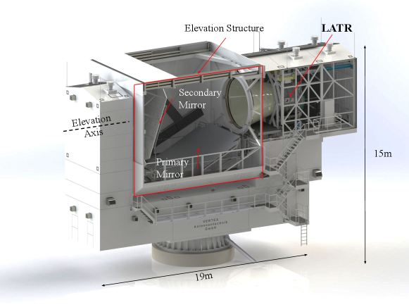
The Simons Observatory (SO) is a next generation ground-based millimeter wavelength survey located at an elevation of 5200 meters on Cerro Toco in the Atacama Desert of northern Chile. It is designed to produce deep temperature and polarization maps of the CMB. The observatory will ultimately consist of six 0.42 m small-aperture telescopes (SATs, (Galitzki et al., 2024)) and one large-aperture telescope (LAT). The LAT (Figure 1) features a crossed-Dragone optical design, with a 6 m primary mirror and a 5.4 m secondary mirror. This optical design allows for a large focal plane occupied by the Large Aperture Telescope Receiver (LATR), covering a 6.7^∘ field of view (Niemack, 2016; Gudmundsson et al., 2021). At the time of writing, construction of the first three SATs and the LAT is complete.

The LAT will survey 40% of the sky with arcminute resolution, sharing significant overlap with surveys in other wavelengths, such as the Dark Energy Spectroscopic Instrument (DESI) (DESI Collaboration et al. (2016)) and the Legacy Survey of Space and Time (LSST) survey of the Vera C. Rubin Observatory (Željko Ivezić et al. (2019)). The complementary datasets these instruments will produce can be used to constrain the lensing potential and the upper bound of the neutrino mass. Similar to ACT and SPT, the LAT will enable temperature and polarization maps. SO is expected to detect over 16,000 galaxy clusters through the thermal SZ effect, over 24,000 extragalactic point sources (The Simons Observatory Collaboration et al., 2019), and a variety of different transient events (Li et al., 2023; Orlowski-Scherer et al., 2024).

In this paper, we start with an overview of the instrument design (Section 2). We then discuss the in-lab cryogenic validation efforts (Section 3) and readout validation tests (Section 4). In Section 5, we describe the instrument’s response to different environmental tests. Finally, in Section 6 we show initial results of testing conducted during the integration of the telescope and receiver.

Refer to caption — Figure 1: A rendered cross-sectional view of the LAT (Zhu et al., 2021). The telescope yoke sits on an azimuth cone (bottom) and supports the elevation structure. The LATR is located in the receiver cabin (upper right), where it can co-rotate with the elevation structure and collect light reflected from the 5.4 m secondary mirror (left). See Figure 10 for a recent photograph of the LAT.

2 LATR Design

We will briefly review the LATR design here; for a more comprehensive treatment, please refer to Zhu et al. (2021). Many of the design details described in the following sections are informed by the experiences of earlier CMB receivers (e.g. ACTPol (Thornton et al., 2016)).

2.1 Cryogenic and Mechanical Design

The LATR consists of five cryogenic stages (80 K, 40 K, 4 K, 1 K and 100 mK) and a 300 K vacuum shell (Figure 2). The receiver utilizes superconducting transition edge sensors (TES) designed to operate at 100 mK (McCarrick et al. (2021)), which acts as the primary driver of the LATR’s cryogenic design. Large temperature variations at the 100 mK stage can induce thermal noise or even risk heating the TESs out of their transition phase, so a stable cold stage is also important for detector performance.

At warmer stages, the desire to balance the LATR’s mechanical robustness against its cryogenic requirements inform many of the design decisions for the cryostat. Mechanical and thermal design study simulations were conducted to optimize the LATR’s mechanical design (Orlowski-Scherer et al., 2018), as were simulations estimating the time to reach the cryogenic operating temperatures (Coppi et al., 2018). Minimizing the cooldown time significantly reduces the logistical challenges when operating in the field and increases the on-sky integration time.

The 300 K stage consists of a front plate, a cylindrical vacuum shell, and a dome-shaped back plate. The front plate contains 13 hexagonal cutouts for anti-reflection coated windows, behind which are mounted infrared blocking filters. The vacuum shell contains flanges for vacuum lines and pressure gauges, as well as insertion ports for the cryogenic refrigerators and readout harnesses. The external ribs of the vacuum shell are also used to mount several components of the readout hardware (Section 2.2.2). The 80 K stage consists of a 2.1 m diameter filter plate, and a short 80 K shell. It is cooled by two PT-90¹¹1https://bluefors.com/products/cryomech-products/ pulse tube cryocoolers, which are coupled to the filter plate via oxygen-free high conductivity (OFHC) copper straps, manufactured by Technology Applications, Inc.²²2https://www.techapps.com/ In order to reduce the total thermal load at 80 K, the entire stage is wrapped in 30 layers of multi-layer insulation (MLI). The 80 K stage mounts to the 300 K vacuum shell via a ring of G10 tabs.

The 40 K stage (highlighted in green in Figure 2) consists of a filter plate, an extended shell, and a back lid. As with the 80 K stage, it is also mounted to the inside of the 300 K vacuum shell through a ring of G10 tabs and is wrapped with 30 layers of MLI. The 4 K stage (highlighted in purple in Figure 2) consists of a filter plate, a radiation shell, and a back lid. It is mounted directly to the 40 K stage through a second ring of G10 tabs. While the optics tubes (OTs) mount directly to the 4 K plate, the majority of their 4 K mass protrudes into the 40 K cavity. To minimize radiative heating, we wrap these 4 K sections of the OT in aluminized Mylar. The 40 K and 4 K stages are cooled by two dual-stage PT-420¹ pulse tube cryocoolers, with each stage coupled to the respective pulse tube stages with custom OFHC braided copper straps. As with the 300 K shell, both the 40 K and 4 K shells interface with the inserted universal readout harness (URH) assemblies via rectangular cutouts (Moore et al., 2022).

The 1 K stage and 100 mK stage are coupled to the still and mixing chamber stages of a Bluefors LD400 dilution refrigerator (DR)³³3https://bluefors.com/, respectively. Mechanically, the two stages share similar designs. In order to transfer cooling power from the DR to the OTs, we utilize a hexagonal OFHC copper back-up structure (BUS). The BUS contains cutouts to minimize its overall mass while maintaining sufficient thermal conductance, and it is coupled to the DR stages via sets of braided, gold-plated OFHC copper straps⁴⁴4https://www.techapps.com/. On each BUS, we bolt copper rods (“cold fingers”) that protrude towards each OT. From there, another copper braided strap connects to a similar OT cold finger, completing the thermal path from the DR’s mixing chamber to the OT. The 1 K cold stage, which is coupled to the DR’s still stage, follows a similar structure. The two BUSes are mechanically connected by a carbon fiber truss. The 1 K BUS is mounted to the 4 K filter plate via six sets of carbon fiber tripods.

In order to preserve structural integrity while maintaining thermal isolation across stages, we use several sets of G10 tabs and carbon fiber trusses. Because of the importance of their functionality, these G10 tabs and carbon fiber trusses in the LATR were subjected to a series of weight tests and pull tests to assess their robustness. After over 20 cooldowns and the LATR’s shipment to Chile, visual in-situ inspection of the G10 tabs and carbon fiber trusses revealed no damage, giving us confidence in their future performance (Orlowski-Scherer, in prep.).

2.2 Readout and Detector Design

The fully populated LATR will field $\sim$ 62,000 TESs across 13 OTs. SO LAT deployment will be broken up into two phases: the first phase will install seven OTs into the LATR, and the second phase (referred to as Advanced Simons Observatory, or ASO) will install the final six OTs. Each OT will contain three universal focal plane modules (UFMs) of identical frequency bands.The UFMs are distributied across the following frequency bands: low-frequency (LF, with center frequencies of 27 and 39 GHz), mid-frequency (MF, with center frequencies of 93 and 145 GHz) and ultra-high-frequency (UHF, with center frequencies of 225 and 280 GHz). The MF and UHF UFMs package $1756$ detectors per array (with $36$ of those being dark detectors, (Duff et al., 2024)). At time of writing, the LF UFM is still being developed and is expected to package between 222 and 244 detectors per wafer. To read out this large volume of TESs, SO employs microwave multiplexing ( $\mu$ Mux, (McCarrick et al., 2021)) where each TES is coupled to a resonator on a transmission line via a RF superconducting quantum interference device (SQUID). This architecture allows for the ability to install $10^{3}$ resonators on a single transmission line (Figure 3). MF UFM performance is reported on in detail in Dutcher et al. (2024).

2.2.1 Cold Readout

A single UFM contains $\sim$ 1800 resonators, and is read out with two sets of transmission lines, with $\sim$ 900 resonators coupled to each line (Figure 3). Resonator frequencies span from 4 to 6 GHz. Additionally, each UFM has a single low frequency DC connection, used to transmit voltage biases to the TESs and flux ramping signals for the SQUIDs. Each OT contains three UFMs, and must support all the cabling and connectors necessary to read them out. To avoid strongly thermally coupling the different OT cold stages, the OT employs a combination of copper-nickel (CuNi) semi-rigid coaxial lines for input lines and niobium titanium (NbTi) coaxial lines for output lines. The CuNi coaxial lines provide attenuation for incoming signals, while the NbTi lines maintain a high signal to noise ratio for the outgoing tones. For the same reason, the DC bias ribbon cables are made from low thermal conductivity NbTi wire.

Outside the OTs, readout lines are connected to the URH at 4 K via isothermal, meter-long copper coaxial cables and DC ribbon cables. The URH is a multi-stage readout insert that carries RF transmissions, flux ramp signals, and DC bias voltages between the 4 K stage and the 300 K stage. Within the URH we utilize CuNi coaxial lines, and PhBr DC ribbon cables which terminate at a routing board on the 40 K stage. Each routing board splits off bias signals to 40 K low-noise amplifiers (LNAs) on the output RF lines. The remaining low frequency signals (i.e., flux ramps, detector biases, and 4 K LNA biases) are routed down to the 4 K stage via additional PhBr wiring and connectors. An analogous routing board is installed on the back of the OT at 4 K, with a corresponding 4 K LNA. While the LNAs are required on the output lines, cryogenic attenuators are required on the input lines to reduce the amount of power dropped on the resonators. The coaxial connections terminate with SMA connectors at 300 K (Moore et al., 2022; Sathyanarayana Rao et al., 2020). The full cold RF readout chain is diagrammed in Figure 4.

2.2.2 Warm Readout

SO utilizes SLAC Microresonator Radio Frequency (SMuRF) electronics (Yu et al. (2023), Henderson et al. (2018)) to read out LATR detectors. Each MF and UHF UFM is read out through a single SMuRF system, with six SMuRF systems populating an Advanced Telecommunications Computing Architecture (ATCA) electronics crate⁵⁵5https://comtel-online.com/. Because LF detectors require larger on-array coupling optics, LF UFMs contain fewer detectors than their MF or UHF counterparts. For this reason, three LF UFMs are read out via a single SMuRF system. For seven OTs, the LATR will deploy 19 SMuRF systems across four crates.

A single SMuRF system consists of five integrated boards: one carrier card, one Rear Transition Module (RTM) card, two Advanced Mezzanine Cards (AMC), and one cryostat card (or “cryocard”). Two AMCs are seated within one carrier card, with an RTM attached to the rear of the carrier card. All of these components are installed in a single ATCA crate slot. The RTM is responsible for generating the low frequency signals: the TES bias voltage, the flux ramp sawtooth signals, and the cryogenic LNA bias voltages. The AMCs generate the RF tones that are sent to the resonators through the coaxial lines, from 4 to 6 GHz. The cryocard relays the low frequency signals from the RTM to the cryostat via the URH. Finally, there is a room temperature LNA installed on the 300 K side of the output lines of the URH, for further amplification.

The cryocard is housed in a separate RF-protected enclosure, which is mounted directly above the URH on the LATR’s 300 K shell. The SMuRF crates are mounted on racks directly on the ribs of the LATR’s vacuum shell. This mechanical arrangement minimizes the length of coaxial lines between the URH 300 K plate and the AMC, reducing total signal loss and ambient coupling (Silva-Feaver et al., 2022).

2.3 Optical Design

Light reflected off the LAT’s secondary mirror enters the LATR through thirteen 3.175 mm thick anti-reflection (AR) coated ultra-high molecular weight polyethylene windows mounted to the 300 K front plate. Mounted behind the windows on the 300 K front plate is a double-sided infrared blocking filter (DSIR). The DSIRs are installed to reduce optical loading on the colder stages (Ade et al., 2006).

On the 80 K filter plate, we install another DSIR and an AR-coated alumina filter. The alumina filters are designed to act as prisms refracting incoming light into the OTs, allowing the OTs to be co-linear with the entire LATR. The central OT has a flat alumina filter, while the inner and outer rings of OTs have increasingly larger sloped gradients, sloping towards the cylindrical axis of the instrument. For reference, the focal plane of the two-mirror crossed-Dragone system is curved, and the edge rays are thus not parallel with the central axis of the OTs (Dicker et al., 2018). The prism shape of the alumina filters here enables a flat detector focal plane. Between the DSIR and the alumina filter, the 80 K stage absorbs a large quantity of optical loading (see Section 3). At 40 K, there is one additional DSIR.

The remaining optical elements are mechanically integrated into the OTs (Figure 5). At 4 K, there is a thick IR blocker, a low-pass edge (LPE) filter, and an AR coated silicon lens. The LPE helps reduce optical loading from out-of-band sources. The silicon lenses are designed to re-image light from the LAT’s focal plane onto the OTs’ focal plane baseplates (FPB). At 1 K, there is a second lens, a Lyot stop and series of baffles (covered in injection molded, carbon-loaded plastic tiles (Xu et al., 2021)), and a final, third lens. At 100 mK we install an LPE, and finally the UFMs. The UFMs contain gold-plated aluminum feedhorns, directly mounted in front of ortho-mode transducers (OMTs) that couple radiation to the TESs. The original cold optical design (Dicker et al., 2018; Gudmundsson et al., 2021) included another LPE at 1 K, but MF OT holography measurements revealed an excess of side-lobe power sourced by this LPE. Follow-up measurements of this OT without the LPE concluded that optical loading and bandpass specifications could still be satisfied without the filter, leading to the decision to leave it out in the final deployment configuration (Sierra et al., 2024).

2.4 LATR Performance Specifications

LATR design decisions were motivated by the requirement to cool the UFMs down to 100 mK. All thermal specifications for the individual cold stages were driven by this requirement. For the warmer stages, the largest concern was about the effect of thermal radiation on colder stages, particularly within the cold optical filter stack. In Tables 1 and 2, we report temperature requirements for the various LATR stages. Thermal simulations suggested that higher temperatures at 80 K would have a minimal effect on the 100 mK stage, so its associated maximum acceptable temperature is quite high (Hill et al., 2018). The reported 4 K stage requirement describes the temperature of the OT’s 4 K filter (right-most optical element in Figure 5). While these temperature stages are not expected to directly affect detector performance, we were concerned that they could potentially warm the 100 mK stage through radiative power. The pulse tube load curves are fairly flat in the regime close to their nominal temperatures listed in Tables 1 and 2. Moreover, the conductivity of aluminum increases with temperature between 40 and 4 K (Woodcraft & Gary, 2009), further alleviating the effect of increased load. Therefore, we only require that the 80, 40, and 4 K loads be under the expected PT capacity to achieve specification. Specifications for 1 K are driven by cooling loop performance in the DR unit. We budgeted $2.85\times 10^{-3}$ W for the 1 K stage and $66.5\times 10^{-6}$ W for the 100 mK stage (Zhu et al., 2021).

3 Cryogenic Validation

The LATR has previously been shown to meet cryogenic design specifications with a single, dark OT installed (Zhu et al. (2021)). In this configuration, no OT lenses, filters, or UFMs were installed. The addition of these elements introduces new sources of thermal loading that require characterization. Through incremental testing, we find that the LATR will still meet cryogenic requirements with 13 fully assembled OTs installed, as listed in Tables 2 and 1.

As mentioned in Section 2.1, any time spent cooling the LATR on the telescope is time taken away from science operations, implying that faster cooldowns can lead to deeper maps. Before turning on any pulse tubes, we pump the LATR out to $10^{-3}$ mbar. In North America, the LATR typically pumps down to the base level pressure within four days, depending on humidity. At the site, where atmospheric pressure is roughly half of what it is at sea level, it takes just under three days to pump out. Once fully pumped out, the cryostat reaches a temperature of 4 K within four days. After reaching 4 K, we start condensing the ³He–⁴He mixture in the DR, which brings the 100 mK stage down to its base temperature within hours. In sum, once completely assembled at the Chilean site, the LATR (without any OTs) can reach base temperature within a week. Based on incremental testing (by adding more OTs during in-lab testing), we estimate that each OT adds $\sim 0.5$ days to the cooldown time. Therefore, we project that the fully assembled and evacuated LATR (with 13 OTs) will take roughly 10 – 11 days to reach base temperature. All temperatures reported in this paper are recorded via a custom, open-source data acquisition framework (Koopman et al., 2020).

3.1 100 mK

Zhu et al. (2021) showed that a single dark OT, without optical elements and UFMs installed, added $<4\,\mu$ W of loading at 100 mK. Additionally, we find that the 100 mK thermal BUS adds $20\,\mu$ W of power. We subsequently performed several cooldowns in various configurations, integrating mechanical, optical, and electronic components as they became available. Ultimately, we were able to assemble an entire OT (with all its respective optical and electronic components, and unbiased detectors) and found the total load of a single OT to be $\leq 6\,\mu$ W, with the FPB temperature to be 54 mK. With this loading, we estimated the FPB temperature in a 13 OT cooldown to be $\geq 91$ mK.

At 100 mK, we budgeted $5\,\mu$ W of total loading per OT; measured values from the test above suggests a higher loading than expected. In order to address this, we introduced another set of heat straps between the 100 mK BUS and the DR to improve the thermal conductivity between them, and hence reduce the gradient induced by the higher loading levels.

In our final in-lab cooldown, we installed two fully assembled, optically-coupled OTs with the extra set of heat straps, and we estimated the 100 mK loading to be 10 $\mu$ W (on top of the $20\,\mu$ W from the thermal BUS). In order to test the new heat strap set-up, we assumed that each OT would add 5 $\mu$ W, and applied 65 $\,\mu$ W to a single resistive heater mounted to the 100 mK BUS to simulate a full 13 OT configuration. At this loading, the DR mixing chamber rose to 40 mK. However, the gradient across the DR straps was only 15 mK (compared to 25 mK with a single heat strap). After extrapolating and assuming the worst gradient from the BUS to the OT FPB based on measurements from previous cooldowns, we estimate that the hottest FPB temperature for a 13 OT configuration would be 80 mK and the BUS temperature would be 55 mK. This is comfortably below our 100 mK requirement listed in Tables 1 and 2.

In 2024, we integrated the LATR with six optically coupled OTs with the LAT. We present the results of cryogenic testing for this cooldown in Section 6.

3.2 80K/40K/4K

In addition to tracking the loading at 100 mK, we also estimated the loading at 80, 40, and 4 K, and made similar extrapolations to 13 OTs.

The 80 K stage’s performance is largely independent from the rest of the receiver, and thus the easiest to characterize. In Table 1, we show that with 7 sets of filters, the filter plate is well under 80 K. Assuming the gradient across the 80 K plate scales linearly with the number of filters, extrapolations to the 13 OT configuration using this data suggest that the hottest part of the 80 K filter plate reaches 85 K, which is under the specification listed in Table 1.

The 40 and 4 K loading is shown in Table 2. Since we employ a dual-stage PT-420 pulse tube here, the performances of these two stages are coupled. This leads to some degeneracy in the measured loading values and contributes to the uncertainties reported in Table 2. Additionally, we installed components as they were obtained; for this reason, the configurations reported in Table 2 are not necessarily well-defined. For example, the 1 OT setup includes one OT, one URH, and three filter sets at 40 K, meaning that from the perspective of 4 K, this is a 1 OT cooldown, while from the perspective of 40 K, it is a 3 OT cooldown. The 40 and 4 K loading is not strictly linear with number of OTs due to slightly differing numbers of available readout cables between OTs. This is a small effect, and to a good approximation, we can estimate the 13 OT loading as:

\text{q}_{13}=\text{q}_{\text{dark}}+\frac{13}{7}(\text{q}_{7}-\text{q}_{\text{dark}}),

(1)

where $q_{dark}$ represents loading in a zero OT configuration. This results in a loading estimate of $66\pm 2$ W and $1.7\pm 0.2$ W at 40 and 4 K, respectively. The 40 K loading is somewhat higher than budgeted (Zhu et al., 2021), while the 4 K loading is lower than budgeted. Both are, however, significantly less than the 40 and 4 K capacities of 110 W and 4 W, respectively. As such we have qualified the 40 and 4 K stages for 7 OTs and forecast that they will also meet specifications for 13 OTs, as described in Tables 1 and 2.

Configuration	Filter Plate Temperature	Loading
Budgeted	$<$ 120 K	180 W
Dark	37-39 K	22 ${}^{+1}_{-1}$ W
2 Filters	40-43 K	35 ${}^{+1}_{-1}$ W
3 Filters	44-47 K	42 ${}^{+1}_{-1}$ W
7 Filters	48-58 K	88 ${}^{+1}_{-1}$ W
13 Filters*	63-85 K	144 ${}^{+1}_{-1}$ W
6 OTs	40-48 K	47 ${}^{+1}_{-1}$ W

Table 1: Budget and estimates of 80 K loading. The first row (“Budgeted”) are informed by performance specfications (Zhu et al., 2021). The number of filters in the configuration column refer to the number of 300 K windows, 300 K DSIRs, and 80 K DSIRs that are installed. Values for the asterisked configuration come from an estimate by extrapolation of measured values, using Equation 1. The “Filter Plate Temperature” describes the range of temperatures measured across the entire filter plate, where the coldest temperature is at one of the pulse tube cryocooler. The final row (“6 OTs”) details the most recent cryogenic measurements from the LATR, with a different filter stack than the other rows; see Section 6 for more details.

Configuration	4 K Plate Temperature	4 K Loading	40 K Plate temperature	40 K Loading
Budgeted	$<$ 8 K	4.0 W	$<$ 55 K	110 W
Dark	2.7 - 5.0 K	$0.9^{+1}_{-1}$ W	$27-47$ K	$33^{+1}_{-1}$ W
1 OT	2.9 - 5.3 K	$1.0^{+0.1}_{-0.1}$ W	$27-48$ K	$34^{+1}_{-1}$ W
3 OT	2.9 - 5.4 K	$1.1^{+0.1}_{-0.1}$ W	$28-49$ K	$38^{+1}_{-1}$ W
7 OT	3.0 - 6.3 K	$1.3^{+0.1}_{-0.1}$ W	$30-53$ K	$51^{+1}_{-1}$ W
13 OT*	$>$ 3.5 K	$1.7^{+0.2}_{-0.2}$ W	$>$ 31 K	$66^{+2}_{-2}$ W
6 OTs	3.0 - 6.3 K	$0.7^{+0.2}_{-0.2}$ W	32 - 52K	$61^{+1}_{-1}$ W

Table 2: Budget and estimates of 4K̇ and 40 K Loading. The dark setup features no OTs, no URHs, and no filter sets. The first row (“Budgeted”) are informed by performance specfications (Zhu et al., 2021). The “1 OT” setup includes one OT, one URH, and three filter sets. The “3OT” setup includes three OTs, one URH, and two filter sets. The “7OT” setup includes seven OTs, two URHs, and seven filter sets. The values in the final row (“13OT”) represent estimates, from extrapolations based on measurements from the first several rows of this table. The ”Plate Temperature” column describes the range of temperatures measured across the entire filter plate, where the coldest temperature is at one of the pulse tube cryocooler. The final row (“6 OTs”) details the most recent cryogenic measurements from the LATR, with a different filter stack than the other rows; see Section 6 for more details.

3.3 Thermal Stability

Thermal fluctuations on the UFMs can lead to high 1/ $f$ noise levels and, in some cases, a loss of resonator tracking. In order to avoid this, the LATR’s 100 mK stage must remain as thermally stable as possible. In a static state, the OT FPBs have been shown to be stable to millikelvin levels (Bhandarkar et al., 2022). However, when overbiasing detectors, the loading at the 100 mK stage jumps by 500 nW per array (Wang et al., 2022; Dutcher et al., 2024). This is a sudden increase in power on the cold stage, but as seen in Figure 6, the cold stage recovers to a stable operating temperature in 5 minutes. When UFMs are biased into their transitions, the load falls to 150 nW per UFM. Detector specifications require thermal fluctuations on the UFMs to be $\leq 500$ $\mathrm{\mu K}$ over 5 minutes. After allowing detectors to settle following biasing, we find the root-mean-square of the UFM temperature across any five minute time period to be $\sim 310$ $\mathrm{\mu K}$ . Here, we take the 12 minute mark in Figure 6 to indicate the start of the stable period.

3.4 TES response vs Bath Temperature

TES bolometers are sensitive to changes in the temperature of the $100$ mK stage of the cryostat to which they sink power ( $T_{\mathrm{bath}}$ ). To maintain equilibrium, the power coming into the TES, including the photons it measures and electrical heating from the TES bias, must match the power flowing out to the bath, which depends on the temperature difference between the TES and $T_{\mathrm{bath}}$ . To first order, small variations in $T_{\mathrm{bath}}$ look like signal in the detector timestreams.

The coupling factor – measured in $\mathrm{pA/mK}$ or $\mathrm{pW/mK}$ – between changes in $T_{bath}$ and detector signal can be calculated from known detector properties, including the thermal conductivity between the TES and the bath and TES gain (which depends on bias level (Irwin & Hilton (2005))).

Other parts of the detector and readout system are also temperature sensitive, such as the resonators in the readout chain or the impedance of the (non-superconducting) coax. The TESs will also slightly vary in gain (current response to incoming power) with changes in $T_{\mathrm{bath}}$ . However, the dominant response to changes in $T_{\mathrm{bath}}$ should be the apparent signal picked up in the TESs. Understanding this coupling also has implications for stability requirements on $T_{\mathrm{bath}}$ while operating and for data processing (see Section 3.3).

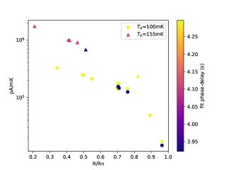
To determine the coupling factor, we designed a test to vary $T_{\mathrm{bath}}$ by varying the power on a resisitve heater mounted on the OT’s FPB. For our initial in-lab testing, we installed a high conductance single pixel box (SPB), with 6 TESs. Testing with an SPB allowed for small-scale detector and readout testing, before scaling up to deployment-grade UFMs. With a function generator, we powered the heater with a long period (45 s) sine wave, in order to give time for the thermal mass of the FPB to respond to the change in power on the resistor. From this test, we estimated a coupling factor of order $10^{6}\,\mathrm{pA/mK}$ , which was consistent with predictions (Figure 7).

However, we note that the high conductance nature of the SPB is not representative of deployment-grade UFMs. Once we had installed UFMs into the LATR, we ran similar tests to determine the coupling factor. For these tests, we incrementally increased the temperature of the UFMs while recording time-ordered data (TODs). While detectors were biased to 50% $R_{N}$ , we measured the coupling factor to be $0.025$ $\mathrm{pW/mK}$ , .

We note that there is a difference in units presented here (pW vs. pA). During SPB testing, we were primarily focused on validating readout noise. Current units are a helpful gauge for this, and much of our infrastructure was designed to test this. However, as we advanced to full-scale detector testing, power units became more important and relevant. Thus, when we tested UFMs, we took measurements in units of pW.

During LATR testing, we were concerned about the effect telescope motion may have on the receiver’s cryogenic environment. This concern motivated the measurements and tests described in this section; because we could not directly measure the effect of LAT motion before LAT/LATR integration, characterizing and constraining the effect of changes to $T_{bath}$ helped manage this risk. In Section 6, we will describe the effect of LAT motions on the LATR’s cryogenic and detector systems.

4 Readout and Detector Validation

Following cryogenic validation, we focused on testing the LATR’s readout system. Characterizing the detector system and understanding the contributions of environmental effects to readout and detector noise prior to on-sky observations was critical in the receiver’s validation efforts. For the baseline detector properties presented in this section, the OT was closed off with an aluminum plate at 4 K. Thus, all the UFMs were exposed to 4 K radiation.

For each cooldown, the LATR readout chain is subject to a litany of checks before closing up: continuity checks are conducted for each DC line, every 4 K and 40 K LNA is biased to check functionality, and the RF chain is looped back at the 4 K stage on the URH. For this last check, we check the 3 GHz to 9 GHz coaxial transmission from 300 K to 4 K with a vector network analyzer (VNA). This warm transmission measurement is useful for checking cable loss and poor coaxial connections. Each UFM bias line and flux ramp line is probed for short or open circuits twice; once before installation into the OT, and once after being fully integrated in an OT. After the OT is installed in the LATR, the full readout chain is connected, from the URH’s 300 K stage to the UFMs on OT’s 100 mK FPB. In this stage of assembly, we can probe the bias lines one last time; however, we cannot make warm RF transmission measurements once the resonators are installed, because the resistance of the niobium traces on the devices is too large to make RF transmission measurements at room temperature. Finally, we connect SMuRF systems and run basic system health checks on the warm hardware.

Once all physical connections and SMuRF systems pass their health checks, we cool the LATR down and start the detector tuning and biasing processes. To begin, we run a full transmission sweep and identify all the resonators (this often includes estimating and setting amplifier biases and in-line attenuation values). We then start tracking resonators, which allows us to monitor TES current for changes in absorbed power. At this point, we are able to stream data and estimate noise-equivalent currents (NEI), providing us with useful information about system performance. If superconducting detector noise is consistent with expectations, we then begin biasing the TESs. This involves running I-V load curves, where we drive the detectors normal by overbiasing them and then slowly step the bias value down to zero. This brings the TESs through their transition regime and provides us with the values of desired bias voltages for operations (typically at 50% $R/R_{N}$ , where $R_{N}$ is the normal resistance of the TES). After setting up detectors initially, we cache all relevant parameters and refer to those values when re-tuning. Typically, these values do not change greatly during a single cooldown. Therefore, caching values cuts out some of the initial set-up steps and minimizes the time spent setting up detectors if the need to re-tune or re-bias comes up. All the processes described here are relayed to the SMuRF hardware via custom software.⁶⁶6https://github.com/simonsobs/sodetlib^,⁷⁷7https://github.com/slaclab/pysmurf

4.1 Baseline Noise

Initial validation of the LATR’s readout system was conducted with an SPB containing 66 RF resonators (Xu et al. (2020)). The simplicity of the SPB enabled straightforward baseline characterization of the readout chain; it allowed us to understand basic properties of the readout system (such as cable loss) while avoiding the confusion introduced from a large number of detector channels. Six of the 66 resonators in the SPB are coupled to prototype TESs, allowing us to test the DC bias chains as well. Testing of the SPB showed that the LATR’s readout chain was performing as expected, in terms of RF noise and DC continuity.

Following SPB testing, we integrated UFMs in to the LATR and continued baseline testing. An MF UFM is designed to support 1756 TESs, but it will never have 100% yield rates when testing and fielding these devices. For each UFM, SO aims to field detectors at a $\geq 70\%$ end-to-end yield, with an ultimate goal of $80\%$ (McCarrick et al., 2021; Dutcher et al., 2024). In Table 3 we list the measured detector yields for six UFMs installed in the LATR. Yield is determined by observing the TES responses to I-V load curves. TES that do not respond to I-V curves correctly are cut and are not a part of the reported yield counts. In Table 3, we show that the first six deployed UFMs meet this specification. UFM Mv11 has a noticeably lower yield; this is due to an open bias line that was discovered after LATR assembly. We know that there are 135 TES associated with this bias line, and the yield rate across the other eleven bias lines on Mv11 is $79.8\%$ .

Array	Test Yield	LATR Yield	Yield Rate
Mv11	1275	1265	72.0%
Mv21	1381	1459	83.1%
Mv24	1497	1543	87.9%
Mv25	1582	1592	90.7%
Mv26	1567	1580	90.0%
Mv28	1442	1440	82.0%

Table 3: Detector yield for LATR MF UFMs during dark testing. Test yield indicates yield from the pre-deployment screening in a test cryostat (Dutcher et al., 2024). LATR yield represents the TES yield measured in the LATR while in the field. Note that the yield for Mv11 is much lower than the other UFMs due to an open bias line, which we plan to repair. Yield rate is calculated for the LATR Yield with respect to the total number of TES per UFM, 1756.

Because LATR cooldowns are lengthy, full-scale initial in-lab UFM screening and testing happens in a test cryostat before installation in the LATR (Wang et al. (2022)). This process delivers baseline noise and efficiency measurements that can be compared with the LATR’s in-situ measurements for validation purposes. Noise-equivalent power (NEP) measurements serve as our principal check for LATR UFM noise properties. Through the software mentioned in Section 4, we directly measure NEI for devices under test. NEP is then calculated as the following (Irwin & Hilton (2005)):

NEP=NEI\frac{1}{|s_{i}|},

(2)

where $s_{i}$ is the responsivity of the TES, determined through bias-steps or I-Vs (Wang et al. (2022)). In Figure 8, we plot the NEPs for a single biased MF UFM and show that the majority of TESs meet the dark baseline specification set for SO, derived from SO instrument forecasting models (McCarrick et al., 2021; The Simons Observatory Collaboration et al., 2019). The vertical dotted lines in Figure 8 represent the baseline dark specifications for each MF frequency: 14.12 $\mathrm{aW/\sqrt{Hz}}$ for 90 GHz, and 25.36 $\mathrm{aW/\sqrt{Hz}}$ for 150 GHz. Future studies will be able to comment on LAT on-sky detector noise, as well as LF and UHF arrays.

5 In Lab Environmental Testing

5.1 Vibrations

To characterize the LATR response to vibrations, we ran a series of shake tests to determine vibrational pickup within the LATR. We were initially concerned that vibrational pickup would have the largest impact in the form of readout noise, but we discovered that the larger effect was thermal. In fact, any effect seen in the detector system is a response to thermal changes induced by vibrations. We mounted a ButtKicker Mini Concert transducer⁸⁸8https://thebuttkicker.com/ to the flange of the LATR’s front plate, and used it to produce vibrations at frequencies supplied via a tone generator. Testing shows that the most noticeable amount of vibrational pickup came in at the 100 mK stage, in the 26 Hz range, although there are peaks at frequencies from 21–24 Hz as well (Figure 9).

Based on simulations and our benchtop thermal BUS testing, we determined that the most likely mode of vibrations was a drum-like feature, where the largest amplitude of vibrations occur at the center of the BUS. To mitigate this, we bolted a copper bar across one axis of the hexagonal BUS, hoping to stiffen any drum-like mode. Testing showed that we did not completely eliminate the mode, but still reduced the amplitude of the thermal change.

As a part of factory acceptance testing of the LAT prior to its installation in Chile, we measured the vibrational environment of the receiver cabin during test scans. To do so, we installed an accelorometer to the front flange of a LATR mass dummy in the telescope and performed scans. Testing showed that the LAT’s primary resonant frequency while scanning was at 3 Hz. This finding was in agreement with pre-fabrication design studies. At higher frequencies, we found minimal power while scanning. Since most of our in-lab LATR tests raised concerns for resonant frequencies above 20 Hz (Figure 9), we concluded that the LATR would not experience vibrational heating when installed in the LAT. To alleviate concerns about the 3 Hz mode, we manually excited a 3 Hz mode on the LATR with a hammer in the lab, and saw no resultant heating. It is worth noting that any testing we conducted involved inducing more vibrational power on the LATR than it would ever actually experience in the LAT. For this reason, we are confident that any vibrational coupling in the telescope would not result in the large thermal changes shown in Figure 9. In Section 6, we show that the LATR does not experience significant heating during LAT scans due to vibrations in the system.

5.2 Ambient RF

6 LATR and LAT Integration

Though the LAT structure has been erected at its site in Chile (Figure 10), as of August 2024 the primary and secondary mirrors have yet to be fully assembled and integrated. In order to proceed with LAT characterization, we opted to install the LATR (with two MF OTs) in the LAT, with aluminum blanks installed at the 4 K stage of the OTs in August 2023. Without the blank and mirrors, the TESs would be saturated and thus unusable for testing. However, with the blanks installed, we are able to bias the TESs into transition and take dark scans while monitoring detector performance.

Figure 11a shows noise performance of LATR detectors during a constant elevation scan (solid lines), with the LAT moving at 1 deg/s with a throw of $60^{\circ}$ and an average turnaround acceleration $1$ deg/s² for $\sim 1$ week, as well as noise performance with the telescope stationary (dashed lines). These scans mimic the expected scan strategy for LAT science observation, so the high degree of agreement between the noise while scanning and while stationary, with very little disagreement between the two sets of auto-spectral densities, indicates the instrument will be stable during operations. Scans are organized, written and commanded via custom observatory control software (Koopman et al., 2024). The peak at 50 Hz is a result of AC power, and the peaks at 1.4 Hz and 2.8 Hz are caused by the pulse tube cryocoolers used by the LATR. The low frequency noise is mostly common mode signal, and $\sim 99\%$ can be removed by subtracting off a common mode modeled using singular value decomposition (SVD) (Figure 11b). This is a promising sign for future on-sky observations, as the LAT plans to perform maximum likelihood map-making with a noise modeling scheme similar to that of ACT, which uses SVD derived modes to model the noise (Dünner et al., 2012).

As seen in Figure 12, most detectors have a white noise level below what we predict from forecasted sensitivity simulations, and NEP medians are comparable to pre-deployment screening values (Dutcher et al., 2024). This implies that the derived values for LAT sensitivities used in forecasting will be achievable once the LAT is taking on-sky observations. The forecasted sensitivities were calculated using BoloCalc (Hill et al., 2018), a sensitivity calculator that takes into account detector properties, bandpasses, the transmission and loading of all elements in the optical chain, and a model of the atmosphere at the SO site. Wherever possible, such as with the bandpasses, we use in-lab measurements for these values (Sierra et al., 2024).

As mentioned in Section 5, detector performance is strongly linked to thermal stability at the 100 mK stage. For this reason, we were concerned about the effect LAT movement may have on cold stage temperatures, and thus, on detector performance. In Figure 13a, we can see the effect of LAT scanning movement on the cold stages of the LATR. All temperature responses that are recorded during LAT scans are sub-percent level. We also note that at turnarounds in LAT scans, there are no significant spikes in temperature, which was a concern prior to integration. To further illustrate this, we plot the temperature of an UFM as a function of azimuth (in Figure 13b) during constant elevation scans. The total measured peak-to-peak temperature during these scans is $\sim 0.25$ mK. The turnarounds are represented by the vertical dotted-lines in this plot; we see no major temperature spikes at those azimuths, implying that the turnarounds do not disrupt the cryogenic environment of the UFM. Based on our test results from Section 3.4, we found the coupling factor to be 0.025 pW/mK. Applying this conversion to the measured peak-to-peak temperature from above yields $6.25$ x $10^{-3}$ pW as the maximum power seen by the detectors from the thermal fluctuations. Assuming a 10 K sky and using the baseline BoloCalc conversion for this configuration (Table 4), we expect sky loading will be $\sim 0.43$ pW at 90 GHz and $\sim 0.59$ pW at 150 GHz. Therefore, the power from temperature fluctuations is at the sub percent level even with a relatively low sky loading.

We also note that the detectors are not affected by LAT turnarounds. For our scan strategy, we expect a turnaround to occur every $120$ s, or at a rate of roughly $0.008$ Hz. In the inset plot of Figure 11a, we see no noticeable peak at that frequency, indicating the detectors are agnostic to turnarounds.

Figure 14 is a dark map we derived from the TODs recorded during LAT scans. Because we are not mapping an actual sky signal, we choose to follow a filter-and-bin mapmaking approach to produce this map, where we simply bin the common mode subtracted TODs into a map. When collecting on-sky data, we will utilize a maximum likelihood (ML) mapmaker. By using the filter-and-bin method, we can derive the map from the TODs faster on the limited compute capabilities at the high elevation site. These maps display variations in the noise levels that correspond to areas of uneven sky coverage and have white noise levels in good agreement with our TODs; see Haridas et al. (2024) for a more complete treatment.

Configuration	90 GHz	150 GHz
Capped at 4K	20.13	14.19
Open to 10K Sky	23.44	16.92

Table 4: K/pW conversions from BoloCalc using SO baseline values (Hill et al., 2018). For example, for the 90 GHz detectors, we expect the sky signal of 10 K to result in 0.43 pW of power at the detectors. This is well-below the saturation power (

P_{sat}

) of SO TES, which are designed to be 2.62 pW for 90 GHz detectors and 7.18 pW for 150 GHz detectors.

Following dark testing of two MF OTs, we installed four more OTs into the LATR (2 MF and 2 UHF). In anticipation of mirror installation, we removed any metal blanks installed at the cryogenic stages. Finally, during site integration, we noticed imperfections in several of the DSIRs that were meant to be installed in the LATR. This led us to replace all DSIRs with several layers of radio-transparent multi-layer insulation (specifically Zotefoam). At 300 K (directly behind the window), we installed two $1/8$ ” layers, one 1” layer, seven more $1/8$ ” layers. At 80 K, we installed three more $1/8$ ” layers. Finally, at 40 K, we installed two $1/8$ ” layers. Zotefoam was selected to replace the filters for spectral and thermal reasons (Choi et al., 2013; Ade et al., 2022). After this switch, we found the thermal loading values below 40 K to be consistent with prior configurations, but we noticed a larger effect at the 40 K and 80 K stages. Specifically: we found $\sim$ 47 W at the 80 K stage, $\sim$ 65 W at the 40 K stage, and $\sim$ 0.7 W at the 4 K stage. The 1 K and 100 mK stages were agnostic to this change (we estimate 6.5 $\mu$ W of loading per OT at 100 mK). Comparing these values to those from prior cooldowns (see Tables 1 and 2), we note that there is far more loading at 40 K and less loading at 80 K in this current configuration. We are currently investigating this change further. Because we do not see a large change in thermal power at the 100 mK stage, we are comfortable with moving forward using this configuration. Initial Fourier transform spectroscopy indicates that the switch to Zotefoam filters has no impact to MF bandpass, with further analysis on the performance of the UHF OTs underway. Additionally, we report on the performance of the recently installed UFMs in Satterthwaite et al. (2024).

7 Conclusion and Future Plans

The Large Aperture Telescope Receiver (LATR) has been integrated into the Simons Observatory (SO) Large Aperture Telescope (LAT) in the Atacama Desert of Chile. The LATR’s cryogenic stages have been shown to meet the desired thermal performance requirements in both the laboratory and the LAT. We also show that the thermal performance of the cold optical elements meets its requirement as well. Additionally, the LATR’s readout and detector chains have been fully characterized in a dark configuration, and we expect that the detector performance will be suitable for on-sky observations.

We expect the LAT’s mirrors will be completed and installed in 2025. At the time of writing, there are six OTs (four MF, two UHF) installed in the LATR in Chile (Haridas et al., 2024; Satterthwaite et al., 2024). The final seven OTs are undergoing development, and are expected to be installed by 2027. In preparation for this final installation, we are exploring minor upgrades to the LATR, in order to improve cryogenic performance. First, as mentioned in Section 6, we replaced our DSIR filters with Zotefoam filters. We will continue to investigate the optical and cryogenic effects of this change. Additionally, previous studies have found that the thermal straps employed in the LATR are not qualified for sub-kelvin performance (Dhuley et al., 2020). While the vendor who produced the LATR’s straps press-welds the copper braids, we believe that electron-beam welding or press welding this interface may greatly improve their performance. We are currently investigating the feasibility and efficacy of these upgrades.

8 Acknowledgements

This work was supported in part by a grant from the Simons Foundation (Award #457687, B.K.). This work was supported by the National Science Foundation (UEI GM1XX56LEP58).

9 CRediT Roles

We list here the roles and contributions of the authors according to the Contributor Roles Taxonomy (CRediT)⁹⁹9https://credit.niso.org/.

Tanay Bhandarkar: Conceptualization (equal), Data curation (equal), Formal analysis (lead), Investigation (lead), Methodology (equal), Resources (equal), Software (equal), Validation (lead), Visualization (equal), Writing - original draft (lead), Writing - review & editing (lead).
Gabriele Coppi: Conceptualization (supporting), Investigation (supporting), Methodology (supporting), Resources (supporting), Writing - review & editing (supporting).
Thomas Satterthwaite: Conceptualization (supporting), Formal analysis (equal), Investigation (equal), Methodology (supporting), Validation (supporting), Writing - review & editing (supporting).
Shawn Henderson: Conceptualization (supporting), Investigation (supporting), Methodology (supporting), Project administration (supporting), Resources (supporting), Software (supporting), Validation (supporting), Writing - review & editing (supporting).
Federico Nati: Conceptualization (supporting), Funding acquisition (lead), Investigation (supporting), Methodology (supporting), Resources (supporting), Validation (supporting), Writing - review & editing (supporting).
Matthew Koc: Conceptualization (supporting), Investigation (supporting), Methodology (supporting), Resources (supporting), Validation (supporting).
Carlos Sierra: Conceptualization (supporting), Investigation (supporting), Methodology (supporting), Resources (supporting), Validation (supporting).
Michael Link: Conceptualization (supporting), Investigation (supporting), Methodology (supporting), Resources (supporting), Validation (supporting), Writing - review & editing (supporting).
Tammy Lucas: Conceptualization (supporting), Investigation (supporting), Methodology (supporting), Resources (supporting), Validation (supporting), Writing - review & editing (supporting).
Michael Vissers: Conceptualization (supporting), Investigation (supporting), Methodology (supporting), Resources (supporting), Validation (supporting).
Kyuyoung Bae: Conceptualization (supporting), Investigation (supporting), Methodology (supporting), Resources (supporting), Validation (supporting).
Shannon Duff: Conceptualization (supporting), Investigation (supporting), Methodology (supporting), Resources (supporting), Validation (supporting), Writing - review & editing (supporting).
Jenna Moore: Conceptualization (supporting), Investigation (supporting), Methodology (supporting), Resources (supporting), Validation (supporting), Writing - review & editing (supporting).
Tran Tsan: Conceptualization (supporting), Methodology (supporting), Software (supporting), Validation (supporting), Writing - review & editing (supporting).
Liam Walters: Conceptualization (supporting), Validation (supporting), Writing - review & editing (supporting).
Jason Austermann: Conceptualization (supporting), Resources (supporting), Validation (supporting), Writing - review & editing (supporting).
Eve Vavagiakis: Conceptualization (supporting), Resources (supporting), Validation (supporting), Writing - review & editing (supporting).
Zeeshan Ahmed: Conceptualization (supporting), Formal analysis (supporting), Funding acquisition (supporting), Investigation (supporting), Methodology (supporting), Project administration (supporting), Resources (supporting), Supervision (supporting), Writing - review & editing (supporting).
Brian Koopman: Conceptualization (supporting), Software (supporting), Writing - review & editing (supporting).
Nicholas Galitzki: Conceptualization (supporting), Methodology (supporting), Writing - review & editing (supporting).
Daniel Dutcher: Conceptualization (supporting), Investigation (supporting), Methodology (supporting), Resources (supporting), Software (supporting), Validation (supporting), Writing - review & editing (supporting).
Mark Devlin: Conceptualization (supporting), Funding acquisition (lead), Investigation (supporting), Methodology (equal), Project administration (lead), Resources (lead), Supervision (lead), Writing - review & editing (supporting).
Robert Thornton: Conceptualization (supporting), Investigation (supporting), Methodology (supporting), Project administration (supporting), Resources (supporting), Validation (supporting), Writing - review & editing (supporting).
Simon Dicker: Conceptualization (supporting), Investigation (supporting), Methodology (supporting), Resources (supporting), Validation (supporting), Writing - review & editing (supporting).
John Orlowski-Scherer: Conceptualization (supporting), Formal analysis (supporting), Investigation (supporting), Methodology (supporting), Validation (supporting), Writing - review & editing (supporting).
Yuhan Wang: Conceptualization (supporting), Data curation (equal), Formal analysis (supporting), Investigation (supporting), Methodology (supporting), Resources (supporting), Software (supporting), Validation (supporting), Writing - review & editing (supporting).
Anna Kofman: Conceptualization (supporting), Formal analysis (supporting), Investigation (supporting), Methodology (supporting), Resources (equal), Software (supporting), Validation (supporting), Visualization (supporting), Writing - review & editing (supporting).
Saianeesh Haridas: Conceptualization (supporting), Data curation (equal), Formal analysis (equal), Investigation (supporting), Methodology (equal), Resources (equal), Software (equal), Validation (supporting), Visualization (supporting), Writing - original draft (supporting), Writing - review & editing (supporting).
Jon Gudmundsson: Conceptualization (supporting), Resources (supporting), Validation (supporting), Visualization (supporting), Writing - review & editing (supporting).
Karen Perez Sarmiento: Conceptualization (supporting), Data curation (supporting), Investigation (supporting), Methodology (supporting), Software (supporting), Validation (supporting), Writing - original draft (supporting).
Mario Zannoni: Conceptualization (supporting), Funding acquisition (supporting), Investigation (supporting), Methodology (supporting), Resources (supporting), Validation (supporting), Writing - review & editing (supporting).
Michele Limon: Conceptualization (supporting), Investigation (supporting), Methodology (supporting), Project administration (supporting), Supervision (supporting), Validation (supporting), Visualization (supporting).
Suzanne Staggs: Conceptualization (supporting), Funding acquisition (supporting), Methodology (supporting), Project administration (supporting), Resources (supporting), Supervision (supporting), Validation (supporting).
Michael Niemack: Conceptualization (supporting), Funding acquisition (supporting), Methodology (supporting), Project administration (supporting), Resources (supporting), Supervision (supporting), Validation (supporting), Writing - review & editing (supporting).

References

Abazajian et al. (2015) Abazajian, K., Arnold, K., Austermann, J., et al. 2015, Astroparticle Physics, 63, 66, doi: https://doi.org/10.1016/j.astropartphys.2014.05.014
Ade et al. (2006) Ade, P. A. R., Pisano, G., Tucker, C., & Weaver, S. 2006, in Millimeter and Submillimeter Detectors and Instrumentation for Astronomy III, ed. J. Zmuidzinas, W. S. Holland, S. Withington, & W. D. Duncan, Vol. 6275, International Society for Optics and Photonics (SPIE), 62750U, doi: 10.1117/12.673162
Ade et al. (2022) Ade, P. A. R., Ahmed, Z., Amiri, M., et al. 2022, The Astrophysical Journal, 927, 77, doi: 10.3847/1538-4357/ac4886
Aghanim et al. (2020) Aghanim, N., Akrami, Y., Ashdown, M., et al. 2020, Astronomy and Astrophysics, 641, A6, doi: 10.1051/0004-6361/201833910
Bhandarkar et al. (2022) Bhandarkar, T., Bhimani, S., Coppi, G., et al. 2022, in Millimeter, Submillimeter, and Far-Infrared Detectors and Instrumentation for Astronomy XI, ed. J. Zmuidzinas & J.-R. Gao, Vol. 12190, International Society for Optics and Photonics (SPIE), 1219012, doi: 10.1117/12.2629557
Bleem et al. (2020) Bleem, L. E., Bocquet, S., Stalder, B., et al. 2020, The Astrophysical Journal Supplement Series, 247, 25, doi: 10.3847/1538-4365/ab6993
Carlstrom et al. (2011) Carlstrom, J. E., Ade, P. A. R., Aird, K. A., et al. 2011, PASP, 123, 568, doi: 10.1086/659879
Choi et al. (2013) Choi, J., Ishitsuka, H., Mima, S., et al. 2013, Review of Scientific Instruments, 84, 114502, doi: 10.1063/1.4827081
Coppi et al. (2018) Coppi, G., Xu, Z., Ali, A., et al. 2018, in 2018SPIE10708, ed. J. Zmuidzinas & J.-R. Gao, Vol. 10708, International Society for Optics and Photonics (SPIE), 246 – 258, doi: 10.1117/12.2312679
Dahal et al. (2022) Dahal, S., Appel, J. W., Datta, R., et al. 2022, The Astrophysical Journal, 926, 33, doi: 10.3847/1538-4357/ac397c
DESI Collaboration et al. (2016) DESI Collaboration, Aghamousa, A., Aguilar, J., et al. 2016, The DESI Experiment Part I: Science,Targeting, and Survey Design. https://arxiv.org/abs/1611.00036
Dhuley et al. (2020) Dhuley, R. C., Posen, S., Geelhoed, M. I., Prokofiev, O., & Thangaraj, J. C. T. 2020, Superconductor Science Technology, 33, 06LT01, doi: 10.1088/1361-6668/ab82f0
Dicker et al. (2018) Dicker, S. R., Gallardo, P. A., Gudmundsson, J. E., et al. 2018, in 2018SPIE10700, ed. H. K. Marshall & J. Spyromilio, Vol. 10700, International Society for Optics and Photonics (SPIE), 1064 – 1076, doi: 10.1117/12.2313444
Duff et al. (2024) Duff, S. M., Austermann, J., Beall, J. A., et al. 2024, Journal of Low Temperature Physics, doi: 10.1007/s10909-024-03117-x
Dutcher et al. (2024) Dutcher, D., Duff, S. M., Groh, J. C., et al. 2024, Journal of Low Temperature Physics, 214, 247, doi: 10.1007/s10909-023-03045-2
Dünner et al. (2012) Dünner, R., Hasselfield, M., Marriage, T. A., et al. 2012, The Astrophysical Journal, 762, 10, doi: 10.1088/0004-637x/762/1/10
Galitzki et al. (2024) Galitzki, N., Tsan, T., Spisak, J., et al. 2024, The Astrophysical Journal Supplement Series, 274, 33, doi: 10.3847/1538-4365/ad64c9
Gudmundsson et al. (2021) Gudmundsson, J. E., Gallardo, P. A., Puddu, R., et al. 2021, Appl. Opt., 60, 823, doi: 10.1364/AO.411533
Haridas et al. (2024) Haridas, S. K., Ahmed, Z., Bhandarkar, T., et al. 2024, The Simons Observatory: Dark Characterization of the Large Aperture Telescope. https://arxiv.org/abs/2407.09669
Henderson et al. (2018) Henderson, S. W., Ahmed, Z., Brown, D., et al. 2018, in Millimeter, Submillimeter, and Far-Infrared Detectors and Instrumentation forAstronomy IX, ed. J. Zmuidzinas & J.-R. Gao (SPIE), doi: 10.1117/12.2314435
Hill et al. (2018) Hill, C. A., Bruno, S. M., Simon, S. M., et al. 2018, in Millimeter, Submillimeter, and Far-Infrared Detectors and Instrumentation for Astronomy IX, ed. J. Zmuidzinas & J.-R. Gao (SPIE), doi: 10.1117/12.2313916
Hilton et al. (2021) Hilton, M., Sifón, C., Naess, S., et al. 2021, ApJS, 253, 3, doi: 10.3847/1538-4365/abd023
Irwin & Hilton (2005) Irwin, K., & Hilton, G. 2005, Transition-Edge Sensors (Berlin, Heidelberg: Springer Berlin Heidelberg), 63–150, doi: 10.1007/10933596_3
Kamionkowski et al. (1997) Kamionkowski, M., Kosowsky, A., & Stebbins, A. 1997, Physical Review Letters, 78, 2058, doi: 10.1103/physrevlett.78.2058
Koopman et al. (2020) Koopman, B. J., Lashner, J., Saunders, L. J., et al. 2020, in Software and Cyberinfrastructure for Astronomy VI, ed. J. C. Guzman & J. Ibsen (SPIE), 6, doi: 10.1117/12.2561771
Koopman et al. (2024) Koopman, B. J., Bhimani, S., Galitzki, N., et al. 2024, The Simons Observatory: Deployment of the observatory control system and supporting infrastructure. https://arxiv.org/abs/2406.15703
Li et al. (2023) Li, Y., Biermann, E., Naess, S., et al. 2023, ApJ, 956, 36, doi: 10.3847/1538-4357/ace599
Madhavacheril et al. (2024) Madhavacheril, M. S., Qu, F. J., Sherwin, B. D., et al. 2024, ApJ, 962, 113, doi: 10.3847/1538-4357/acff5f
McCarrick et al. (2021) McCarrick, H., Healy, E., Ahmed, Z., et al. 2021, The Astrophysical Journal, 922, 38, doi: 10.3847/1538-4357/ac2232
Moore et al. (2022) Moore, J. E., Bhandarkar, T., DiGia, B., et al. 2022, in Millimeter, Submillimeter, and Far-Infrared Detectors and Instrumentation for Astronomy XI, ed. J. Zmuidzinas & J.-R. Gao, Vol. 12190, International Society for Optics and Photonics (SPIE), 1219025, doi: 10.1117/12.2630527
Niemack (2016) Niemack, M. D. 2016, Appl. Opt., 55, 1688, doi: 10.1364/AO.55.001688
Orlowski-Scherer (in prep.) Orlowski-Scherer, J. in prep., Review of Scientific Instruments
Orlowski-Scherer et al. (2024) Orlowski-Scherer, J., Venterea, R. C., Battaglia, N., et al. 2024, The Astrophysical Journal, 964, 138, doi: 10.3847/1538-4357/ad21fe
Orlowski-Scherer et al. (2018) Orlowski-Scherer, J. L., Zhu, N., Xu, Z., et al. 2018, in 2018SPIE10708, ed. J. Zmuidzinas & J.-R. Gao, Vol. 10708, International Society for Optics and Photonics (SPIE), 644 – 657, doi: 10.1117/12.2312868
POLARBEAR Collaboration et al. (2020) POLARBEAR Collaboration, Adachi, S., Faúndez, M. A. O. A., et al. 2020, The Astrophysical Journal, 897, 55, doi: 10.3847/1538-4357/ab8f24
Sathyanarayana Rao et al. (2020) Sathyanarayana Rao, M., Silva-Feaver, M., Ali, A., et al. 2020, Journal of Low Temperature Physics, 199, 807, doi: 10.1007/s10909-020-02429-y
Satterthwaite et al. (2024) Satterthwaite, T. P., Ahmed, Z., Bae, K., et al. 2024, in Society of Photo-Optical Instrumentation Engineers (SPIE) Conference Series, Vol. 13102, Society of Photo-Optical Instrumentation Engineers (SPIE) Conference Series, ed. J. Zmuidzinas & J.-R. Gao, 1310223, doi: 10.1117/12.3019196
Sierra et al. (2024) Sierra, C. E., Harrington, K., Sutariya, S., et al. 2024, Simons Observatory: Pre-deployment Performance of a Large Aperture Telescope Optics Tube in the 90 and 150 GHz Spectral Bands, doi: 10.48550/arXiv.2405.06868
Silva-Feaver et al. (2022) Silva-Feaver, M., Ahmed, Z., Arnold, K., et al. 2022, in Millimeter, Submillimeter, and Far-Infrared Detectors and Instrumentation for Astronomy XI, ed. J. Zmuidzinas & J.-R. Gao, Vol. 12190, International Society for Optics and Photonics (SPIE), 121900U, doi: 10.1117/12.2629024
The Simons Observatory Collaboration et al. (2019) The Simons Observatory Collaboration, 2019, JCAP, 2019, 056, doi: 10.1088/1475-7516/2019/02/056
Thornton et al. (2016) Thornton, R. J., Ade, P. A. R., Aiola, S., et al. 2016, ApJS, 227, 21, doi: 10.3847/1538-4365/227/2/21
Wang et al. (2022) Wang, Y., Zheng, K., Atkins, Z., et al. 2022, Journal of Low Temperature Physics, 209, 944, doi: 10.1007/s10909-022-02870-1
Woodcraft & Gary (2009) Woodcraft, A., & Gary, A. 2009, AIP Conference Proceedings, 1185, 681, doi: 10.1063/1.3292433
Xu et al. (2020) Xu, Z., Bhandarkar, T., Coppi, G., et al. 2020, in Millimeter, Submillimeter, and Far-Infrared Detectors and Instrumentation for Astronomy X, ed. J. Zmuidzinas & J.-R. Gao, Vol. 11453, International Society for Optics and Photonics (SPIE), 1145315, doi: 10.1117/12.2576151
Xu et al. (2021) Xu, Z., Chesmore, G. E., Adachi, S., et al. 2021, Applied Optics, 60, 864, doi: 10.1364/ao.411711
Yu et al. (2023) Yu, C., Ahmed, Z., Frisch, J. C., et al. 2023, Review of Scientific Instruments, 94, 014712, doi: 10.1063/5.0125084
Zhu et al. (2021) Zhu, N., Bhandarkar, T., Coppi, G., et al. 2021, The Astrophysical Journal Supplement, 256, 23, doi: 10.3847/1538-4365/ac0db7
Željko Ivezić et al. (2019) Željko Ivezić, Kahn, S. M., Tyson, J. A., et al. 2019, The Astrophysical Journal, 873, 111, doi: 10.3847/1538-4357/ab042c