Signatures of topological phase transition on a quantum critical line
Abstract
Recently topological states of matter have witnessed a new physical phenomenon where both edge modes and gapless bulk coexist at topological quantum criticality. The presence and absence of edge modes on a critical line can lead to an unusual class of topological phase transition between the topological and non-topological critical phases. We explore the existence of this new class of topological phase transitions in a generic model representing the topological insulators and superconductors and we show that such transition occurs at a multicritical point i.e. at the intersection of two critical lines. To characterize these transitions we reconstruct the theoretical frameworks which include bound state solution of the Dirac equation, winding number, correlation factors and scaling theory of the curvature function to work for the criticality. Critical exponents and scaling laws are discussed to distinguish between the multicritical points which separate the critical phases. Entanglement entropy and its scaling in the real-space provide further insights into the unique transition at criticality revealing the interplay between fixed point and critical point at the multicriticalities.
I Introduction
In the quest of classifying novel phases of quantum matter in the absence of local order parameters, the topology of electronic band structure plays a prime role haldane1988model ; kane2005quantum ; narang2021topology ; wang2017topological . It enables the distinction between gapped phases in terms of a quantized invariant number, which counts the number of localized edge modes present thouless1982quantized . The transition between the distinct topological phases involves a bulk band gap closing at the point of topological phase transition. Across the transition the number of edge modes, protected by the bulk gap, changes hasan2010colloquium . In the gapped phases, the localization length of the edge modes diverges as the system drives towards the transition point or criticality continentino2020finite .
Interestingly, this conventional knowledge is revised recently, realizing even criticalities can host the stable localized edge modes despite the vanishing bulk gap verresen2018topology ; verresen2019gapless ; jones2019asymptotic ; verresen2020topology ; rahul2021majorana ; niu2021emergent ; PhysRevB.104.075132 ; PhysRevResearch.3.043048 ; fraxanet2021topological ; keselman2015gapless ; scaffidi2017gapless ; duque2021topological . This results in the emergence of non-trivial criticalities with unique topological properties even in the presence of gapless bulk excitations. The non-trivial criticalities can be effectively characterized in terms of the zeros and poles of complex function associated with the Hamiltonian verresen2018topology . The localized edge modes at criticality are protected by novel phenomena such as kinetic inversion verresen2020topology (in fermionic models) and finite high energy charge gap fraxanet2021topological (in bosonic models). It has been shown that they also remain robust against interactions and disorders verresen2018topology ; verresen2019gapless . This intriguing interplay between topology and criticality causes an unconventional topological transition between critical phases verresen2020topology ; kumar2021multi .
In this work, we report the possibility of a new kind of topological phase transition between critical phases, happening at a multicritical point where two critical lines intersect. Considering a two-band model as a prototype representing gapless (critical) topological insulators and superconductors, in Sec. II, we find the critical lines in the model and existence of two species of multicritical points with quadratic and linear dispersions, both corresponding to the topological transition between distinct critical phases. In support of our finding, in Sec. III, we solve the Dirac equation for criticality to obtain the localized edge mode solutions in the non-trivial critical phases. This is further supported by our proposal of obtaining the non-zero integer winding number for non-trivial critical phases which we discuss in Sec. IV.1. This proposal is supported in Sec. IV.2 by calculating the winding number using zeros and poles of a complex function. The curvature function diverges on approaching the multicritical points from critical phases indicating the existence of a transtion between critical phases. The critical exponents , discussed in Sec. V.1, unravel the different universality classes of two multicritical points. Using the divergence of curvature function we develop a renormalization group (RG) scheme to distinguish the different critical phases in Sec. V.2. In Sec. V.3 we show that a correlation length, extracted from the Fourier-transformed curvature function, diverges at the multicritical points indicating phase transitions between critical phases. Further, in Sec. VI we study the spatial scaling of entanglemet entropy, especially to characterize and distinguish the multicritical points. The scaling reveals an interplay between the fixed points and multicritical points. The entanglement entropy is minimum where the fixed point and multicritical point overlap reflecting the dominance of the former over the latter. Finally, we conclude in Sec. VII .
II Model
We consider a one-dimensional lattice chain of spinless fermions in momentum space PhysRevLett.42.1698 ; kitaev2001unpaired represented by a generic two-band Bloch Hamiltonian of the form
| (1) |
where , and and are the Pauli matrices. The model represents extended Su-Schrieffer-Heeger (SSH) hsu2020topological and extended Kitaev models niu2012majorana by uniquely defining the parameters (see Appendix.A for detailed discussion on the physical relevance of the model). The parameters , and describe the onsite potential, the nearest neighbor (NN) couplings and the next nearest neighbor (NNN) couplings respectively.
In general, the model can support three distinct gapped phases distinguished by the number of edge modes they possess. These phases can be identified with the winding numbers and , which quantify the edge modes. The model undergoes transition between these phases with necessarily involving the gap closing, , at the phase boundaries. The criticalities, where the bulk gap closes, occurs for the momentum , which respectively gives the critical surfaces , and . The model possesses three multicritical lines at which two critical surfaces intersect. Two of them () share identical properties and shows quadratic dispersion around the gap closing point and the other one () is identified with the linear dispersion. Uniquely, the model supports the edge modes and topological transition at critical surfaces corresponding to respectively (see Appendix.B for the numerical results).
To further explore these unique phenomena we propose a framework that works out for criticality without referring to any of the gapped phases of the model. Ideally driving the system to criticality involves and , where is the critical point in the parameter space. To avoid the singularities involving the exact critical point, one can define the Hamiltonian critical only in the parameter space as with , where . This situation is hereafter referred as criticality in this work.
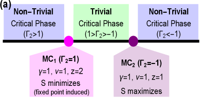
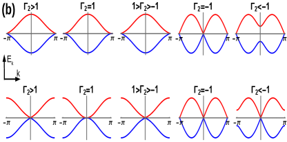
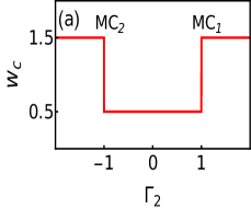
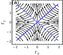
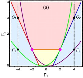
The model at criticality can be obtained by using the critical surface relation which modifies the components into and for and and for . The possible topological trivial and non-trivial critical phases are separated by the phase boundaries at the multicritical lines () and (). Without loss of any generality, we assume . Hence hereafter the critical surfaces and the multicritical lines will be called as the critical lines and the multicritical points respectively, as shown in Fig. 1(a). The multicriticalities, , are identified with quadratic and linear dispersion respectively, as shown in Fig. 1(b). They can be obtained for the following . For ():
| (2) | ||||
| (3) |
For ():
| (4) | ||||
| (5) |
Interestingly, exhibits swapping of the values of . At , one can observe that for which was obtained for and for which was obtained for . This property emerge as a result of intersection of both the critical lines at . We will show in the following that our proposed framework based on the near-critical Hamiltonian can capture the essential physics of topological transition at criticality.
III Bound state solution of the Dirac equation
The presence of edge modes in topological insulators and superconductors is lucid from the bound state solution of Dirac equation jackiw1976solitons ; lu2011non ; shun2018topological . We solve the model in Eq.1 for the bound state solution at criticality (see Appendix.C for the bound state solution at gapped phases). Interestingly, as a consequence of the near-critical approach adopted here, the Dirac Hamiltonian at criticality naturally fixes the interface at a multicritical point. Dirac Hamiltonian at criticality up to third-order expansion around for is
| (6) |
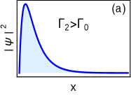
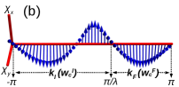
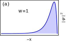
where , and . We look for zero energy solution in real space (we set throughout the discussion), . Identifying the spinor of the wave-function is an eigenstate of and using , inverse of the non-zero decay length can be obtained as . For both roots to be positive, it requires , which implies . The edge mode decay length (longer one of two) is remains finite and positive for i.e., , which means the criticality in this region possesses edge modes and is the topological non-trivial phase. Note that, the term is the gap term at criticality, which mimics the role of mass. As the decay length indicating the edge mode delocalize into the bulk and topological transition takes place at i.e., at . To visualize this phenomenon we write the bound state solution which distributes dominantly near the boundary and decay exponentially as , as shown in Fig.2(a).
To identify the topological transition at and the corresponding topological non-trivial phase one has to consider the swapping property of , which emerge as a result of intersection of critical lines at . In this case, after expanding around and using the swapping property, the Dirac Hamiltonian can be obtained up to second order as
| (7) |
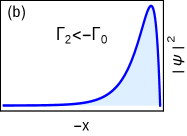
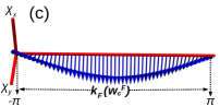
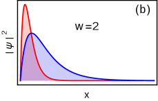
where , and . With , the edge mode decay length is obtained using and is positive if . Therefore, in this case, the gap term is which vanish at the multicritical point , i.e. at . This implies that the criticality is topological non-trivial phase and the topological transition occur at , i.e. as a consequence of the delocalization of edge mode into the bulk as . In this case the bound state solution , distribute near the boundary and decay as as shown in Fig.2(b).
IV Winding number
The topological character of a gapped phase is quantified using topological invariant numbers thouless1982quantized . The quantized values of these invariant numbers represents the number of localized stable edge modes at each end of the open chain. For one dimensional systems winding number is a good invariant number which represents the winding of psuedospin vector in the Brillion zone PhysRevLett.115.177204 .
Therefore, the edge excitations of the gapped phases can be quantified in terms of winding number hasan2010colloquium
| (8) |
where is the Berry connection or curvature function of Bloch wavefunction .
In order to quantify the edge modes at criticality one has to define the winding number at criticality verresen2020topology . The conventional definition of winding number fails at criticalities. This is due to the non-analyticity of the curvature function (integrand in Eq.8) at criticalities. This constraint is naturally avoided in the near-critical approach and allows one to calculate the winding number in its usual integral form even at criticality.
| (9) |
However, it yields fractional values, as shown in Fig.3(a), which does not account correctly for the number of edge modes present at criticalities.
Alternatively, one can refer to the auxiliary space and differentiate between NN and NNN loops and consider only one among them which gives integer contribution and accounts for the edge modes at criticality rahul2021majorana . However, this method is not efficient as the auxiliary space loops gets complicated with the increasesing NN couplings PhysRevLett.115.177204 .
IV.1 Winding number at criticality
The fractional values at criticality imply the presence of fractional winding of unit vector , in the auxiliary space over the Brillouin zone PhysRevLett.115.177204 ; verresen2020topology ; rahul2021majorana . For non-trivial critical phases, one can identify integer winding () of the unit vector along with an extended fractional winding () in the Brillouin zone, as shown in Fig.3(b). For trivial criticalities, only fractional winding can be observed as in Fig.3(c). Based on this, we propose that the winding number at criticality should be approximated to only the integer values which effectively captures the number of edge modes at criticality.
Proposition: Winding number at criticality (), which acquires fractional values (), can be effectively approximated only to its integer part i.e. , to quantify the number of edge modes present at criticality.
The proposal roots in the fact that the momentum zones can be divided into integer and fractional windings as and respectively. The cut-off differentiates the momentum zones responsible for integer and fractional windings of the unit vector, as shown in Fig.3(b). Therefore, we write
| (10) |
The fractional winding can be found to have since the critical phases have one gap closing point in the Brillouin zone. The interger winding counts the number of edge modes in the corresponding critical phase. The winding number in the non-trivial critical phases of the model can be found to have , for which the corresponding . Hence correctly accounts for one edge mode living at the criticalities which we also find from the solution of the Dirac equation. For the trivial critical phase and implying no localized edge modes. The transition between the critical phases with and occur at the multicritical points. This clearly demonstrates the topological transition at criticality through multicritical points.
The proposal can be found viable for the critical systems that support non-trivial critical phases having the winding number and characterized with a single gap closing point. The models with couplings beyond the second neighbor kumar2022topological support the non-trivial critical phases with winding numbers , etc. In the case of , the unit vector winds twice with an extended fractional winding in the Brillouin zone. The approximation to only the integer value yields which counts the two edge modes localized in the corresponding critical phase. Therefore, we expect that the proposition will be useful in characterizing the non-trivial critical phases with higher winding numbers and a single gap closing point. For more than one gap closing point in the Brillouin zone, such as the non-high symmetry points discussed in Ref. kumar2022topological , the proposition might need further modification.
IV.2 Winding number using zeros and poles
The proposal and the integer winding number can be found consistent with the method used in Ref.verresen2018topology , where the winding number is defined using number of zeros () and order of poles (), . The zeros and poles of a complex function is obtained by writing the fermionic creation and annihilation operators in terms of Majorana operators and followed by a Fourier transformation. With the substitution , (where is a complex number) where goes around the unit circle in the complex plane as varies over the Brillouin zone, we get the complex function living on the unit circle in the complex plane
| (11) |
For extended Kitaev model it reads (with no poles) where are respectively (parameters of Kitaev model in Eq.33). Using the mapping , , and one can write the complex function for the generic model
| (12) |
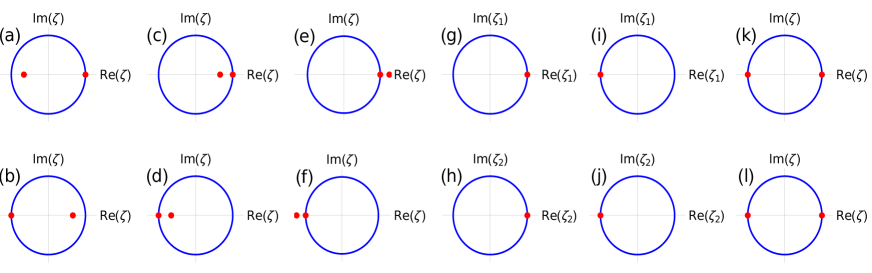
The solutions are . To characterize the topological trivial and non-trivial critical phases we write the solution at criticalities. For we get , and for we get , .
It is evident that one of the zero lie on the unit circle since the system is critical and other zero falls inside (outside) the unit circle for topological non-trivial (trivial) critical phase, as shown in Fig.4. Winding number is determined by the number of zeros falls inside the unit circle, whose value can be found consistent with . For non-trivial critical phases as shown in Fig.4(a,b,c,d) (where upper and lower panels represents respectively), and for trivial critical phases as shown in Fig.4(e,f), .
V Curvature function
Topological phase transition can be induced by changing the underlying topology of the system upon tuning the parameters appropriately. The information of the topological property of the system is embedded in the curvature function defined at momentum chen2016scaling ; chen2016scalinginvariant ; chen2018weakly ; PhysRevB.95.075116 ; chen2019universality ; molignini2018universal ; molignini2020generating ; abdulla2020curvature ; malard2020scaling ; molignini2020unifying ; rufo2019multicritical ; kartik2021topological . The topological quantum phase transition can be identified from the quantized jump of topological invariant number as the parameter tuned across the critical point . As the system approaches critical point to undergo topological phase transition i.e, , curvature function diverges at , with the diverging curve satisfying . The sign of the diverging peak flips across the critical point as
| (13) |
Interestingly, even at criticality, the qualitative behavior of the curvature function remains the same with the fact that, now the critical point is a multicriticality which governs the topological transition between critical phases. As one tunes the parameters at criticality towards a multicritical point , the curvature function diverges at with the symmetric nature , as shown in Fig.5(a).
Topological transition is signalled as the sign of the diverging peak flips if the parameters tuned across the multicritical point.
| (14) |
This is the characteristic feature of topological transition at criticality through both the multicritical points . The curvature function of the generic model at criticality can be written using the critical line relations of the parameters. The pseudo-spin vectors on the two critical lines, , of the model are and . This defines curvature function on the critical lines ,
| (15) |
The property in Eq.14 can be observed to be obeyed by as shown in the Fig.5(b,c,d,e). They show the critical behavior of curvature function around the multicritical points , which distinguish between distinct critical phases. The peak of the curvature function tends to diverge as the parameters approach from both sides at criticality. Both the criticalities exhibit the universal nature of curvature function around the multicritical points.
The scenario around on the critical line shows the divergence in curvature function at the , as shown in Fig.5(b). As the parameter is tuned towards its multicritical value (i.e ) on both sides, the diverging peak of curvature function increases leading to a complete divergence at and flips sign as the critical value is crossed. This signals the topological transition across at criticality. Similar behavior of curvature function can be observed around on the critical line , for which the divergence occurs at , as shown in Fig.5(c).

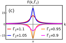
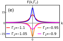
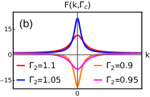
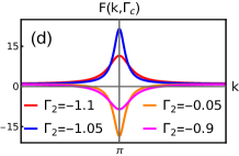
The nature of curvature function around at both the criticalities share the same property of divergence and flipping of sign as shown in Fig.5(d) and 5(e). Note that, the at which the diverging peak increases on approaching the multicritical value, is instead of for (and instead of for ). This swapping of occur as a consequence of the intersection of critical lines. Typically the multicritical point is the same point for both the critical lines in parameter space. These critical lines intersect each other at , which results in the swapping of respective values.
V.1 Critical exponents
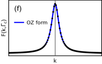
The condition in Eq.13 for curvature function allows one to choose the proper gauge for which can be written in Ornstein-Zernike form around the chen2016scaling ,
| (16) |
where is small deviation from , is the height of the peak and is characteristic length scale or the width of the peak. As we approach critical point, one can also find the divergence in the characteristic length along with the curvature function. The divergences in both and give rise to the critical exponents
| (17) |
where and are the critical exponents which define the universality class of the undergoing topological phase transition. These exponents obeys a scaling law, imposed by the conservation of topological invariant, which reads for 1D systems PhysRevB.95.075116 .
Surprisingly, these scaling behavior of curvature function also appear at multicriticality by approaching it along the critical lines. Approaching multicritical points , curvature function acquires Ornstein-Zernike form around .
| (18) |
where , is the characteristic length scale at criticality and it represents the width of the curvature function that develops around as the parameters . The critical behavior of curvature function around the multicritical points can be captured by the same exponents and defined by
| (19) |
One can calculate these critical exponents and quantify the scaling properties, numerically, through fitting the diverging peak of curvature function with the Ornstein-Zernike form in Eq.18, as shown in Fig.5(f). The data points collected for and can then be fitted again with the equation of the form in Eq.19, to extract the exponents and at the multicritical points. Fig.6(a) and (b) shows the acquired values of exponents for and respectively, on approaching from either sides. The critical exponents are found to be, and for both multicritical points , where and represents the scaling behavior of curvature function with positive (negative) peaks around the multicritical points on both the criticalities.

The exponents can also be estimated analytically by writing the curvature function in Ornstein-Zernike form (see Appendix.D for details). It yield the same values of critical exponents for both . The exponents calculated obeys certain scaling laws and defines universality class of the multicriticalities. For topological transition occurring through both the multicritical point the exponents are found to have both numerically and analytically. The scaling law for 1D systems PhysRevB.95.075116 is thus true for the critical behavior of the multicritical points governing the topological transition at criticality.
In addition, the dynamical exponent dictates the nature of the spectra near the gap closing momenta , i.e. verresen2018topology . It can be calculated numerically as shown in the Fig.6(c) and (d), where the data points around gap closing momenta at the multicritical points are shown. The spectra is quadratic at and linear at . The quadratic spectra results in the dynamical critical exponent , whilst for linear spectra . This behavior is true for both the criticalities. Therefore, the multicriticalities with both and favour the topological transition at criticality.
The universality class for the topological transition at criticality through both can now be obtained using the set of three critical exponents , which captures the scaling behavior around the multicritical points with distinct nature. The universality class of the multicriticality at is and for it reads . Therefore, it is clear that the topological transition at quantum criticality occurs through two distinct multicriticalities which belongs to different universality classes.
V.2 Scaling theory
Based on the divergence of the curvature function, a scaling theory has been developed chen2016scaling ; chen2016scalinginvariant ; chen2018weakly ; chen2019universality ; molignini2018universal ; molignini2020generating ; abdulla2020curvature ; chen2016scaling ; malard2020scaling ; molignini2020unifying ; kumar2021multi . This is achieved by the deviation reduction mechanism where the deviation of the curvature function from its fixed point configuration can be reduced gradually. In the curvature function , for a given in the parameter space, one can find a new which satisfies
| (20) |
where is small deviation away from the , satisfying . As a consequence of the same topology of the system at and at fixed point , the curvature function can be written as , where is curvature function at fixed point and is deviation from the fixed point. The scaling procedure drives the deviation part of curvature function . The fixed point configuration is invariant under the scaling operation i.e., .
Performing the scaling procedure in Eq.20 iteratively and solving for every deviation , one can obtain a renormalization group (RG) equation for the coupling parameters. Expanding Eq.20 in leading order and writing and , one can obtain a generic RG equation
| (21) |
Since the curvature function diverges at , the scaling procedure gradually drives the system away from towards without changing the topological invariant. Thus, eventually, the RG flow distinguishes between distinct gapped phases and correctly captures the topological phase transitions between the gapped phases in the system.
In order to capture the topological transition at criticality one can modify the same scaling scheme to incorporate the multicriticality. This is possible since the qualitative behavior of the curvature function defined at criticality exhibits the same diverging nature near multicritical points with the property (here is small deviation from ). As the parameters at criticality , the topology of the critical phase changes implying a topological transition at multicritical point.
Based on the divergence of the curvature function at criticality, the scaling theory can be achieved by performing the deviation reduction mechanism at criticality. As a consequence of the same topology of the system at and at fixed point , the curvature function can be written as , where is the curvature function at fixed point and is deviation from the fixed point. For a given , one can find a new which satisfies . Iteratively performing this scaling procedure and solving for every , deviation of curvature function decreases and eventually .
One can obtain a renormalization group (RG) equation for the coupling parameters using the scaling parameter and as
| (22) |
The distinct critical phases with different topological characters can be distinguished from the RG flow of Eq.22. The multicritical points and fixed points are then easily captured by analyzing the RG flow lines.
| Multicritical point: | ||||
| Stable fixed point: | ||||
| Unstable fixed point: | (23) |
Performing the RG scheme to the model at criticality, we obtain the RG equations for as
| (24) |
Both the critical lines , yield the same RG equations. The multicritical point is manifested as a line with all flow lines flowing away, as shown in Fig.7(a). The condition in Eq.23 for multicritical points is satisfied as the flow rate diverges at , which also indicate that it is the topological phase transition point between critical phases. Surprisingly, () is obtained as a line of unstable fixed points at which flow rate vanishes with all the flow lines are flowing away.
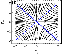
In order to realize the topological transition at criticality through one has to consider the swapping of . The RG equation for the critical line , has to be derived with and vice versa. This procedure yield the RG equations of the form
| (25) |
In this case, () is obtained to be the topological transition point between critical phases, with the diverging flow rate and flow lines directing away, as shown in Fig.7(b). The unstable fixed point appear at () with vanishing flow rate and flow lines flowing away.
V.3 Wannier state correlation function
Along with the RG scheme, a correlation function in terms of Wannier-state representation is proposed to characterize the topological phase transition PhysRevB.95.075116 . This quantity may be measured in higher dimensions chen2019universality ; PhysRevLett.110.165304 ; duca2015aharonov . It is the filled-band contribution to the charge-polarization correlation between Wannier states at different positions, and can be obtained after the Fourier transform of the curvature function. For the two-band model considered here with only the lower band occupied the Wannier state at a distance ,
| (26) |
with position operator , defines Wannier state correlation function as the overlap of the states at the origin and at a distance , as PhysRevB.95.075116
| (27) |
Meanwhile, the substitution of the Ornstein-Zernike form of curvature function (Eq.16) yields the Wannier state correlation function , to be
| (28) |
where can be treated as correlation length of topological phase transition. The correlation function decays exponentially on either sides of the critical point. The decay gets slower as the parameter is tuned towards criticality.
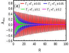
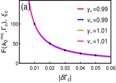
Surprisingly, this notion of correlation function holds true even at criticality and identify the unique topological phase transition at criticality. The behavior of correlation function evidently show that the topological phase transition occurs at the multicritical points at both the criticalities. The Wannier state correlation function can be calculated at criticality as
| (29) |
where for . The correlation function decays faster away from the the multicritical point and the decay slow down as one approaches with the correlation length , as shown in Fig.8(a). Both the criticalities shows same behavior of correlation function near this multicritical point on both sides indicating that the multicriticality is indeed a topological phase transition point at criticality. Note that, the only difference between the criticalities for and is the oscillatory behavior of originating from the term .
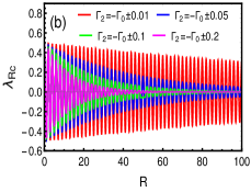
To obtain the critical nature of one has to consider the swapping of (Eq.4 and Eq.5), which yields . This captures the critical nature of , where the decay gets slower as one approaches this point from both the sides, as shown in Fig.8(b). Therefore, the behavior of the correlation function evidently shows that the topological phase transition occurs at the multicritical points. For both the criticalities, the correlation length coinsides with the decay length of the edge modes at criticality studied earlier.
VI Entanglement Entropy
The characteristics of a criticality can be effectively quantified from the entanglement entropy (EE) of the ground state by arbitrarily dividing a system into two subsystems PhysRevLett.90.227902 ; PhysRevLett.102.255701 ; PhysRevLett.121.076802 . Taking the advantage of Wick’s theorem, the eigenvalues of the reduced density matrix can be extracted from the two point correlation matrix, which in the thermodynamic limit can be written as PhysRevLett.121.076802
| (30) |
with (where is the subsystem size). The EE () can be computed as PhysRevLett.121.076802
| (31) |
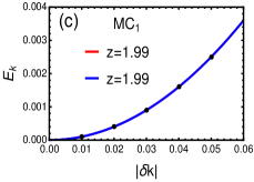
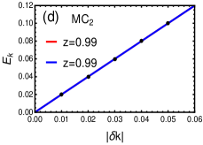
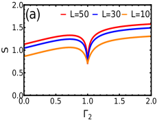
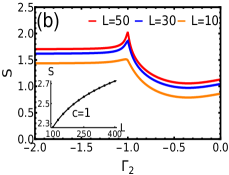
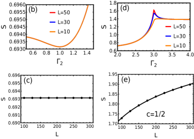
where are the eigenvalues of correlation matrix. The EE signals the topological transition at the multicritical points, as shown in Fig.9. The profile of EE shows, maxima at (Fig.9(b)) and surprisingly minima at (Fig.9(a)).
For the generic model in Eq.1, the is the intersection point of fixed and critical lines. Remarkably, at , we observe that the fixed point characteristic is more dominant which results in the minima of entanglement entropy, in oppose to the critical point behavior where entanglement is supposed to maximize due to the enhanced correlations (see Appendix.E for more details). Besides, at , the bulk is not a CFT. This can be seen from the multiplicity factor () i.e. the degenerate zeros on the unit circle of the complex function associated with the Hamiltonian. The multiplicity at is (see Fig.4(g,h,i,j)). As shown in Ref.verresen2018topology , if the complex function has degenerate zeros with multiplicity , the bulk is not CFT and implies the dynamical exponent . This is consistent with value obtained for (see Fig.6(c)).
At , the EE is PhysRevLett.121.076802 where constant and the central charge as shown in the inset of Fig.9(b). The value of at is consistent with Ref. PhysRevLett.121.076802 , where was found to be the sum of the central charges of intersecting criticalities. As is the intersecting point of the two Ising criticalities (), we get .
VII Conclusion
In this work, we reconstruct various tools to characterize the unusual topological phase transitions between distinct critical phases of an extended model that represents topological insulators and superconductors at criticality. Bound state solutions of the Dirac equation and winding number defined for criticality show that the transitions between the critical phases occur through multicritical points of different universality classes as captured through the critical exponents obtained from the divergence of the curvature function. There exists an interesting swapping behavior of the critical momenta at which manifests in the behavior of curvature function. A scaling theory based on the curvature function unravels that the transitions at can be efficiently identified from the RG flow in the parameter space and also shows that, manifests as unstable fixed line of RG flow for and vice versa. A diverging correlation length obtained from the Wannier state correlation function, which essentially is the Fourier transform of the curvature function, indicates the ocurrences of topological phase transitions at . Moreover, the unique transitions at are characterized with the minima and maxima of entanglement entropy respectively revealing an intriguing dominance of the fixed point over the criticality at .
Our proposed framework, in general, can be applied to the driven systems and higher dimensional systems. A unique advantage of having topological non-trivial criticalities is that the quantum information remains robust upon tuning the system towards it verresen2019gapless . By identifying the multicritical points one can choose a proper criticality to tune into and avoid the decoherence due to bulk gap closing and opening. Our topological model at criticality can be simulated with a good control over the tunable parameters in the suitable experimental platforms which include the superconducting circuit with a single qubit PhysRevB.101.035109 ; niu2021simulation and the ultracold atoms mimicking the topological models goldman2016topological ; xie2019topological ; an2018engineering ; meier2018observation ; meier2016observation , especially the Kitaev model with controlled NN and NNN couplings kraus2012preparing ; jiang2011majorana ; an2018engineering .
Acknowledgements.
We would like to thank Wei Chen, Griffith M. Rufo, Ruben Verresen, Yuanzhen Chen, Aditi Mitra, Vinod N Rao, Randeep N. C for the useful discussions. RRK, YRK and RS would like to acknowledge DST (Department of Science and Technology, Government of India-EMR/2017/000898 and CRG/2021/00996) and AMEF (Admar Mutt Education Foundation) for the funding and support. NR acknowledges Indian Institute of Science (IISc.), Bangalore for support through the Institution of Eminence (IoE) Post-Doc program. This research was supported in part by the International Centre for Theoretical Sciences (ICTS) during a visit for participating in the program - Novel phases of quantum matter (Code: ICTS/topmatter2019/12).Appendix A Physical relevance of model Hamiltonian
The model considered in Eq.1 is a generic two band model for spinless fermions in 1D lattice with nearest neighbor (NN) and next nearest neighbor (NNN) coupling amplitudes of electrons. It maps into extended Su-Schrieffer–Heeger (SSH) PhysRevLett.42.1698 ; hsu2020topological and Kitaev chains kitaev2001unpaired ; niu2012majorana in momentum space, which are the simplest 1D models for topological insulators and superconductors respectively. The tight-binding Hamiltonians can be written as
| (32) |
| (33) |
where and are the fermionic creation and annihilation operators. In , the subscripts denote the sub-lattices, with onsite potential and NN (NNN) hopping amplitude . In , is onsite potential and is NN (NNN) pairing and hopping amplitudes.
The Hamiltonians can be readily diagonalised by Fourier transformation to obtain a generalized Bloch Hamiltonian in the basis of spinor
| (34) |
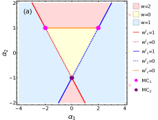
The Hamiltonian , where and . The excitation spectra can be obtained as . The gap closing points (i.e., ) for a specific defines critical surfaces or phase boundaries which separate topologically distinct gapped phases. The gapless edge excitations of these gapped phases are quantified in terms of winding number , which counts the number of edge modes present in the corresponding gapped phases. There are three critical surfaces for extended SSH model. Two of them are with high symmetry nature (i.e, ), and respectively for and . One with non-high symmetry nature (i.e, ), for . Without loss of generality, we assume , hence critical surfaces and multicritical lines will be critical lines and multicritical points respectively on the plane, as shown in Fig.10(a). The three critical lines distinguish the gapped phases with invariant number . There are three multicritical points named (two of them) and , with distinct nature, at which the critical lines meet malard2020multicriticality .
The edge mode remains localized at the criticalities (critical lines) between the topological non-trivial gapped phases ( and ), which give rise to the topological characteristics to the criticality. The same does not occur at the criticality between a trivial and non-trivial gapped phases ( and ). This results in the criticality to get separated into two distinct critical phases with trivial and non-trivial topological properties. The multicritical points , with quadratic (i.e. ) and linear dispersions (i.e. ) respectively, facilitates the topological transition at criticality between trivial and non-trivial critical phases.
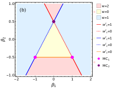
Similar qualitative behavior can also be observed in the extended Kitaev model due to the striking similarity in the phase diagram with SSH model. For the Kitaev model one can obtain
| (35) |
The Hamiltonian , where and , after a rotation along . The gap closing critical surfaces for this case are , and respectively for , and . These phase boundaries separate the gapped phases with invariant numbers as shown in Fig.10(b) (for ). Localized edge modes living at the criticalities between the non-trivial topological gapped phases can be observed here as well which defines trivial and non-trivial critical phases with distinct topological properties. The multicritical points mediate the topological transition at criticality between critical phases with distinct topological nature and share the same properties as in the case of SSH model.
To study the unusual topological transition at criticalities we consider a generic model which essentially summarize both SSH and Kitaev model, thereby giving one platform to study both topological insulator and superconductor models in one dimension. We define a generalized Bloch Hamiltonian for two band model by setting , , and . This model captures the physics of both SSH and Kitaev models, especially the phenomenon of multicriticality and the corresponding topological transition.
Appendix B Numerical results of edge modes and topological transition at criticality
We begin by discussing the behavior of the pseudo spin-vectors to identify the trivial and non-trivial criticalities. The characteristic feature of the parameter space curve at criticality is that it passes through the origin while tracing closed curve. Non-trivial critical phases can be identified with the emergence of secondary loops which encircle the origin indicating a finite winding number or edge modes at criticality, as shown in Fig.11(a). In trivial critical phase parameter space curves always passes through the origin without encircling loops, thus there is no edge modes at criticality, as shown in Fig.11(b).


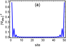
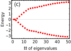
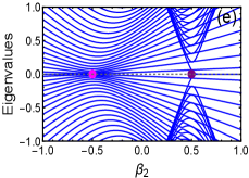
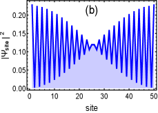
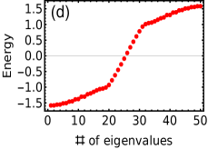
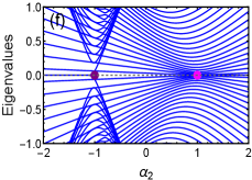
Numerical diagonalization of the Hamiltonians in Eq.32 and Eq.33 (the results shown in this section summerizes both SSH and Kitaev model in open boundary condition) reveals that for the non-trivial critical phases the probability of wave function significantly distributes at the edge of the finite open chain representing the stable localized edge modes, as shown in Fig.12(a). The corresponding eigenvalue distribution shows two of the eigenvalues trapped at zero energy even if there is no bulk gap, as shown in Fig.12(c). In case of the trivial critical phase, probability distribution can be found delocalized over the entire system, as shown in Fig.12(b). Correspondingly, there are no eigenvalues living at zero energy, as shown in Fig.12(d). The localization and delocalization of the edge modes change across the multicritical points which thus differentiate between trivial and non-trivial critical phases.
The topological transition among the non-trivial and trivial critical phases can be identified in the energy spectrum with the system parameter. The presence (absence) of zero energy states dictates the non-triviality (triviality) with respect to the system parameter, as shown in Fig.12(e) and (f). Note that, there is no bulk gap in the spectrum since the system is at criticality. The zero energy states represent localized stable edge modes living at the critical phases. The transition among the trivial and non-trivial phases can be seen at the multicritical points.
Appendix C Bound state solution of Dirac equation for gapped phases
The model Hamiltonian in Eq.1 can be recasted in the form of Dirac Hamiltonian in 1D, which represents the topological insulator and superconductor models. The Dirac Hamiltonian of the model can be obtained by the second order expansion of around the gap closing momenta
| (36) |
For we have , and . For , , and . The continuum version of the model reads (with )
| (37) |
To obtain zero energy solution , we multiply from right-hand side. This implies the wavefunction , is an eigenstate of . The resulting second order differential equation can be written as
| (38) |
We set the trial wavefunction to obtain the secular equation, which yields the inverse of the decay length
| (39) |
The decay length is positive if which identifies the gapped topological non-trivial phase with . Similarly, topological phase with can also be identified by using the ansatz , which under the condition yields the decay length . The decay length is positive if . Even though, the topological trivial phase with is also identified with , it does not host any zero energy solution since the region for trivial phase satisfies the relation . If the parameter , spin distribution of the ground state does not show anti-parallel spin orientation in momentum space shun2018topological . If is satisfied, spin orientation align in the opposite directions with the increasing momentum. Thus the gapped phases and are identified with the condition respectively. The wave-function for zero energy solution can be derived to be
| (40) |
up to normalization constant. The solution is exponentially localized near the boundary, as shown in Fig.13 for different gapped phases.
Appendix D Analytical evaluation of critical exponents
The critical exponents in Section.V.1 can also be estimated analytically by writing the curvature function (Eq.15) in Ornstein-Zernike form. It can be achieved by expanding the pseudo-spin vector around up to third order.
| (41) |
Expansion of the individual components of the vectors and for both the criticalities of the model yields
| (42) | ||||
| (43) | ||||
| (44) | ||||
| (45) |
The expression for is obtained after considering the swapping of . The Ornstein-Zernike form of the curvature function for can be obtained as
| (46) |
where , and . Similarly, for it reads
| (47) |
where , and . Now the critical exponents can be obtained using Eq.19. The exponent is given by
| (48) |
Exponent can be obtained by identifying the dominant term among the coefficients of and . It can be easily seen that approaching multicritical points on both the criticalities yields . This implies
| (49) |
Thus both the numerical and analytical methods yield the same values of critical exponents for topological transition through multicritical points at criticality.
Appendix E Entanglement entropy at critical and fixed points
In order to understand the behavior of EE at the multicritical point , at first, we show is the intersection point of fixed and critical lines in the parameter space. The fixed lines can be obtained by performing the curvature function renormalization group method chen2016scaling , to capture the topological transition between gapped phases of the generic model in Eq.1, in plane with . There are two high symmetry critical lines for respectively. The CRG equations can be obtained as
| (50) | ||||
| (51) |
where the upper and lower signs are for respectively. The critical and fixed lines can be obtained from the CRG equations using the conditions and respectively chen2018weakly , and are depicted in Fig.14(a). From the CRG equations for , the fixed line can be obatined as (purple line), which intersects the critical line (red line) at the multicritical point . Similarly, from the CRG equations for , the fixed line (green line) is obtained and it intersects the critical line (blue line) at the multicritical point . Both the multicritical points are of type as explained in Fig.10. Therefore, it is clear that the is the intersection point of fixed and critical lines.
The EE shows minima at a fixed point in contrast to a critical point (where the EE is maximum), as shown in Fig.14(b,c,d,e). We choose two vertical paths in the parameter space at , as shown in Fig.14(a). The paths intersect the critical points at (i.e. at ) and fixed points at (i.e. at ). The EE shows minima as a consequence of minimal correlations at the fixed points, as shown in Fig.14(b) and subsytem-size independence at the fixed points 14(c). Similarly, the maximum correlations yields the maxima at the critical points, as shown in Fig.14(d). Moreover, at the critical points the EE is where ‘’ is the central charge of the CFT and is a constant. Fig.14(e) shows the scaling of EE at and with , representing Ising criticality verresen2019gapless . In contrast, the fixed points and are in the gapped phase and the EE remains constant with subsystem size representing the area law, as shown in Fig.14(c). This demonstrates the distinction between fixed and critical points in terms of EE and its scaling.
References
- (1) F. D. M. Haldane. Phys. Rev. Lett. 61, 2015 (1988).
- (2) Charles L Kane and Eugene J Mele. Phys. Rev. Lett. 95, 226801 (2005).
- (3) Prineha Narang, Christina A. C. Garcia and Claudia Felser. Nat. Mater. 20, 293–300 (2021).
- (4) Jing Wang and Shou-Cheng Zhang. Nat. Mater. 16, 1062–1067 (2017).
- (5) D. J. Thouless, M. Kohmoto, M. P. Nightingale, and M. den Nijs. Phys. Rev. Lett. 49, 405 (1982).
- (6) M Zahid Hasan and Charles L Kane. Rev. Mod. Phys. 82, 3045 (2010).
- (7) Mucio A Continentino, Sabrina Rufo, and Griffith M Rufo. Finite size effects in topological quantum phase transitions. Strongly Coupled Field Theories for Condensed Matter and Quantum Information Theory, Springer Proceedings in Physics 239 (2020).
- (8) Ruben Verresen, Nick G Jones, and Frank Pollmann. Phys. Rev. Lett. 120, 057001 (2018).
- (9) Ruben Verresen, Ryan Thorngren, Nick G Jones, and Frank Pollmann. Phys. Rev. X. 11, 041059 (2021).
- (10) Nick G Jones and Ruben Verresen. J. Stat. Phys. 175, 1164–1213 (2019).
- (11) Ruben Verresen. arXiv:2003.05453v1 [cond-mat.str-el] (2020).
- (12) S Rahul, Ranjith R Kumar, Y R Kartik, and Sujit Sarkar. J. Phys. Soc. Jpn. 90, 094706 (2021).
- (13) Sen Niu, Yucheng Wang, and Xiong-Jun Liu. arXiv:2106.13400v2 [cond-mat.str-el] (2021).
- (14) Ryan Thorngren, Ashvin Vishwanath, and Ruben Verresen. Phys. Rev. B. 104, 075132 (2021).
- (15) Oleksandr Balabanov, Daniel Erkensten, and Henrik Johannesson. Phys. Rev. Res. 3, 043048 (2021).
- (16) Joana Fraxanet, Daniel González-Cuadra, Tilman Pfau, Maciej Lewenstein, Tim Langen, and Luca Barbiero. Phys. Rev. Lett. 128, 043402 (2022).
- (17) Anna Keselman, Erez Berg. Phys. Rev. B. 91, 235309 (2015).
- (18) Thomas Scaffidi, Daniel E. Parker, Romain Vasseur. Phys. Rev. X. 7, 041048 (2017).
- (19) Carlos M. Duque, Hong-Ye Hu, Yi-Zhuang You, Vedika Khemani, Ruben Verresen, and Romain Vasseur. Phys. Rev. B. 103, L100207 (2021).
- (20) Ranjith R Kumar, Y R Kartik, S Rahul, and Sujit Sarkar. Sci. Rep. 11, 1–20 (2021).
- (21) W. P. Su, J. R. Schrieffer, and A. J. Heeger. Phys. Rev. Lett. 42, 1698–1701 (1979).
- (22) A Yu Kitaev. Phys. Usp. 44, 131 (2001).
- (23) Hsiu-Chuan Hsu and Tsung-Wei Chen. Phys. Rev. B. 102, 205425 (2020).
- (24) Yuezhen Niu, Suk Bum Chung, Chen-Hsuan Hsu, Ipsita Mandal, S Raghu, and Sudip Chakravarty. Phys. Rev. B. 85, 035110 (2012).
- (25) Roman Jackiw and Cláudio Rebbi. Phys. Rev. D. 13, 3398 (1976).
- (26) Jie Lu, Wen-Yu Shan, Hai-Zhou Lu, and Shun-Qing Shen. New J. Phys. 13, 103016 (2011).
- (27) Shun-Qing Shen. Topological Insulators: Dirac Equation in Condensed Matter. Springer (2018).
- (28) G. Zhang and Z. Song. Phys. Rev. Lett. 115, 177204 (2015).
- (29) Ranjith R Kumar, Y R Kartik, and Sujit Sarkar. arXiv:2211.03320 [cond-mat.str-el] (2022).
- (30) Wei Chen. J. Condens. Matter Phys. 28, 055601 (2016).
- (31) Wei Chen, Manfred Sigrist, and Andreas P Schnyder. J. Condens. Matter Phys. 28, 365501 (2016).
- (32) Wei Chen. Phys. Rev. B. 97, 115130 (2018).
- (33) Wei Chen and Andreas P Schnyder. New J. Phys. 21, 073003 (2019).
- (34) Paolo Molignini, Wei Chen, and Ramasubramanian Chitra. Phys. Rev. B. 98, 125129 (2018).
- (35) Paolo Molignini, Wei Chen, and R Chitra. Phys. Rev. B. 101, 165106 (2020).
- (36) Faruk Abdulla, Priyanka Mohan, and Sumathi Rao. Phys. Rev. B. 102, 235129 (2020).
- (37) M Malard, H Johannesson, and W Chen. Phys. Rev. B. 102, 205420 (2020).
- (38) Paolo Molignini, R Chitra, and Wei Chen. Europhys. Lett. 128, 36001 (2020).
- (39) Rufo, S., Lopes, N., Continentino, M.A. and Griffith, M.A.R. Phys. Rev. B. 100, 195432 (2019).
- (40) Y R Kartik, Ranjith R Kumar, S Rahul, Nilanjan Roy, and Sujit Sarkar. Phys. Rev. B. 104, 075113 (2021).
- (41) Wei Chen, Markus Legner, Andreas Rüegg, and Manfred Sigrist. Phys. Rev. B. 95, 075116 (2017).
- (42) Dmitry A. Abanin, Takuya Kitagawa, Immanuel Bloch, and Eugene Demler. Phys. Rev. Lett. 110, 165304 (2013).
- (43) L. Duca, T. Li, M. Reitter, I. Bloch, M. Schleier-Smith, and U. Schneider. Science. 347, 288–292 (2015).
- (44) G. Vidal, J. I. Latorre, E. Rico, and A. Kitaev. Phys. Rev. Lett. 90, 227902 (2003).
- (45) Frank Pollmann, Subroto Mukerjee, Ari Turner, Joel E. Moore. Phys. Rev. Lett. 102, 255701 (2009).
- (46) Daniel Yates, Yonah Lemonik, Aditi Mitra. Phys. Rev. Lett. 121, 076802 (2018).
- (47) Ziyu Tao, Tongxing Yan, Weiyang Liu, Jingjing Niu, Yuxuan Zhou, Libo Zhang, Hao Jia, Weiqiang Chen, Song Liu, Yuanzhen Chen, and Dapeng Yu. Phys. Rev. B. 101, 035109, (2020).
- (48) Jingjing Niu, Tongxing Yan, Yuxuan Zhou, Ziyu Tao, Xiaole Li, Weiyang Liu, Libo Zhang, Hao Jia, Song Liu, Zhongbo Yan, et al. Sci. Bull. 66, 1168–1175 (2021).
- (49) Nathan Goldman, Jan C Budich, and Peter Zoller. Nat. Phys. 12, 639–645 (2016).
- (50) Eric J Meier, Fangzhao Alex An, and Bryce Gadway. Nat. Commun. 7, 1–6 (2016).
- (51) Fangzhao Alex An, Eric J Meier, and Bryce Gadway. Phys. Rev. X. 8, 031045 (2018).
- (52) Dizhou Xie, Wei Gou, Teng Xiao, Bryce Gadway, and Bo Yan. npj Quantum Inf. 5, 1–5 (2019).
- (53) Eric J. Meier, Fangzhao Alex An, Alexandre Dauphin, Maria Maffei, Pietro Massignan, Taylor L. Hughes, and Bryce Gadway. Science 362, 929–933 (2018).
- (54) Liang Jiang, Takuya Kitagawa, Jason Alicea, AR Akhmerov, David Pekker, Gil Refael, J Ignacio Cirac, Eugene Demler, Mikhail D Lukin, and Peter Zoller. Phys. Rev. Lett. 106, 220402 (2011).
- (55) Christina V Kraus, Sebastian Diehl, Peter Zoller, and Mikhail A Baranov. New J. Phys. 14, 113036 (2012).
- (56) Mariana Malard, David Brandao, Paulo Eduardo de Brito, and Henrik Johannesson. Phys. Rev. Res. 2, 033246 (2020).