Signal Processing Meets SGD: From Momentum to Filter
Abstract
In deep learning, stochastic gradient descent (SGD) and its momentum-based variants are widely used for optimization, but they typically suffer from slow convergence. Conversely, existing adaptive learning rate optimizers speed up convergence but often compromise generalization. To resolve this issue, we propose a novel optimization method designed to accelerate SGD’s convergence without sacrificing generalization. Our approach reduces the variance of the historical gradient, improves first-order moment estimation of SGD by applying Wiener filter theory, and introduces a time-varying adaptive gain. Empirical results demonstrate that SGDF (SGD with Filter) effectively balances convergence and generalization compared to state-of-the-art optimizers. The code is available at https://github.com/LilYau350/SGDF-Optimizer.
1 Introduction
During the training process, the optimizer serves as a critical component of the model. It refines and adjusts model parameters to ensure that the model can recognize underlying data patterns. Beyond updating weights, the optimizer’s role includes strategically navigating complex loss landscapes [16] to locate regions that offer the best generalization [30]. The chosen optimizer significantly impacts training efficiency, influencing model convergence speed, generalization performance, and resilience to data distribution shifts [3]. A poor optimizer choice can result in suboptimal convergence or failure to converge, whereas a suitable one can accelerate learning and ensure robust performance [46]. Thus, continually refining optimization algorithms is essential for enhancing the capabilities of machine learning models.
Meanwhile, Stochastic Gradient Descent (SGD) [41] and its variants, such as momentum-based SGD [50], Adam [32], and RMSprop [25], have secured prominent roles. Despite their substantial contributions to deep learning, these methods have inherent drawbacks. They primarily exploit first-order moment estimation and frequently overlook the pivotal influence of historical gradients on current parameter adjustments. Consequently, they can result in training instability or poor generalization [7], especially with high-dimensional, non-convex loss functions common in deep learning [21]. Such characteristics render adaptive learning rate methods prone to entrapment in sharp local minima, which can significantly impair the model’s generalization capability [63]. Various Adam variants [8, 37, 40, 66] aim to improve optimization and enhance generalization performance by adjusting the adaptive learning rate. Although these variants have achieved some success, they still have not completely resolved the issue of generalization loss.
To achieve an effective trade-off between convergence speed and generalization capability [20], this paper introduces a novel optimization method called SGDF (SGD with Filter). SGDF incorporates filter theory from signal processing to enhance first-moment estimation, balancing historical and current gradient estimates. Through its adaptive weighting mechanism, SGDF precisely adjusts gradient estimates throughout the training process, thereby accelerating model convergence while preserving generalization ability.
Initial evaluations demonstrate that SGDF surpasses many traditional adaptive learning rate and variance reduction optimization methods across various benchmark datasets, particularly in terms of accelerating convergence and maintaining generalization. This indicates that SGDF successfully navigates the trade-off between speeding up convergence and preserving generalization capability. By achieving this balance, SGDF offers a more efficient and robust optimization option for training deep learning models.
The main contributions of this paper can be summarized as follows:
-
•
We introduce SGDF, an optimizer that integrates historical and current gradient data to compute the gradient’s variance estimate, addressing the slow convergence of the vanilla SGD method.
-
•
We theoretically analyze the benefits of SGDF in terms of generalization (Section 3.3) and convergence (Section 3.4), and empirically verify the effectiveness of SGDF (Section 4).
-
•
We employ first-moment filter estimation in SGDF, which can also significantly enhance the generalization capacity of adaptive optimization algorithms (e.g., Adam) (Section 4.4), surpassing traditional momentum strategies.
2 Related Works
Convergence: Variance Reduction to Adaptive Methods. In the early stages of deep learning development, optimization algorithms focused on reducing the variance of gradient estimation [2, 13, 27, 48] to achieve a linear convergence rate. Subsequently, the emergence of adaptive learning rate methods [15, 17, 62] marked a significant shift in optimization algorithms. While SGD and its variants have advanced many applications, they come with inherent limitations. They often oscillate or become trapped in sharp minima [54]. Although these methods can lead models to achieve low training loss, such minima frequently fail to generalize effectively to new data [22, 56]. This issue is exacerbated in the high-dimensional, non-convex landscapes characteristic of deep learning settings [11, 39].
Generalization: Sharp and Flat Solutions. The generalization ability of a deep learning model depends heavily on the nature of the solutions found during the optimization process. Keskar et al. [31] demonstrated experimentally that flat minima generalize better than sharp minima. SAM [19] theoretically showed that the generalization error of smooth minima is lower than that of sharp minima on test data, and further proposed optimizing the zero-order smoothness. GAM [65] improves SAM by simultaneously optimizing the prediction error and the number of paradigms of the maximum gradient in the neighborhood during the training process. Adaptive Inertia [55] aims to balance exploration and exploitation in the optimization process by adjusting the inertia of each parameter update. This adaptive inertia mechanism helps the model avoid falling into sharp local minima.
Second-Order and Filter Methods. The recent integration of second-order information into optimization problems has gained popularity [36, 60]. Methods such as Kalman Filter [28] combined with Gradient Descent incorporate second-order curvature information [42, 51]. The KOALA algorithm [12] posits that the optimizer must adapt to the loss landscape. It adjusts learning rates based on both gradient magnitudes and the curvature of the loss landscape. However, it should be noted that the Kalman filtering framework introduces more complex parameter settings, which can hinder understanding and application.
3 Method
We derive SGDF and discovered that it shares the same underlying principles as Wiener Filter [53]. SGDF minimizes the mean squared error [29], which effectively reduces the variance of the estimated gradient distribution. This design ensures that the algorithm achieves a trade-off between convergence speed and generalization. We demonstrate how SGDF intuitively acts. As illustrated in Fig. 1, the property of SGDF to estimate the optimal gradient when the noise of a specific stochastic gradient is very large makes its descent direction more accurate. However, the stochastic gradient descent is affected by the noise, causing the descent path to deviate from the optimal point.
3.1 SGDF General Introduction

In the SGDF algorithm, serves as a key indicator, calculated as the exponential moving average of the squared difference between the current gradient and its momentum , acting as a marker for gradient variation with weight-adjusted by . Zhuang et al. [66] first proposed the calculation of , which is utilized for estimating the fluctuation variance of the stochastic gradient. We derived a correction factor under the assumption that and are independently and identically distributed (i.i.d.), to accurately estimate the variance of using . Fig. 11 compares performances with and without the correction factor, showing superior results with correction. For the derivation of the correction factor, please refer to Appendix A.2.
At each time step , represents the stochastic gradient for our objective function, while approximates the historical trend of the gradient through an exponential moving average. The difference highlights the gradient’s deviation from its historical pattern, reflecting the inherent noise or uncertainty in the instantaneous gradient estimate, which can be expressed as [37].
SGDF utilizes the gain , where the components of each dimension of the estimated gain range between 0 and 1, to balance the current observed gradient and the past corrected gradient , thus optimizing the gradient estimate. This balance plays a crucial role in noisy or complex optimization scenarios, helping to mitigate noise and achieve stable gradient direction, faster convergence, and enhanced performance. The computation of , based on and , aims to minimize the expected variance of the corrected gradient for optimal linear estimation in noisy conditions. For the method derivation, please refer to Appendix A.1.
3.2 Method Principle of Fusion of Gaussian Distributions for Gradient Estimate
SGDF optimizes gradient estimate through the Wiener Filter, enhancing the stability and effectiveness of the optimization process and facilitating faster convergence. By fusing two Gaussian distributions, SGDF significantly reduces the variance of gradient estimates, thereby benefiting in solving complex stochastic optimization problems. In this section, we will delve into how SGDF achieves the reduction of gradient estimate variance.
The properties of SGDF ensure that the estimated gradient is a linear combination of the current noisy gradient observation and the first-order moment estimate . These two components are assumed to have Gaussian distributions, where . Hence, their fusion by the filter naturally ensures that the fused estimate is also Gaussian.
Consider two Gaussian distributions for the momentum term and the current gradient :
-
•
The momentum term is normally distributed with mean and variance , denoted as .
-
•
The current gradient is normally distributed with mean and variance , denoted as .
The product of their probability density functions is given by:
| (1) |
Through coefficient matching in the exponential terms, we obtain the new mean and variance:
| (2) |
The new mean is a weighted average of the two means, and , with weights inversely proportional to their variances. This places between and , closer to the mean with the smaller variance. The new standard deviation is smaller than either of the original standard deviations and , reflecting the reduced uncertainty in the estimate due to the combination of information from both sources. This is a direct consequence of the Wiener Filter’s optimality in the mean-square error sense. The proof is provided in Appendix A.3.
3.3 Generalization Analysis of the Variance Lower Bound for SGDF
In Section 3.2, we explained the principle of noise reduction by SGDF. In this section, we illustrate the advantages of SGDF over other variance reduction techniques, ensuring better generalization.
In prior variance reduction techniques [13, 27, 48], the variance is gradually reduced at a rate of . This approach rapidly decreases the initial variance, facilitating a linear convergence rate, as noted in [5]. However, this approach poses a potential problem in that the variance may approach zero, thus depriving the optimization process of necessary stochastic exploration. The Wiener Filter satisfies statistical estimation theory, wherein the Cramér-Rao lower bound (CRLB) [43] provides an important lower bound of the variance in the estimator. Thus, we construct a dynamical system modeled by the Fokker-Planck equation to demonstrate the potential benefits of having a lower bound on the variance for optimization.
Theorem 3.1.
Consider a system described by the Fokker-Planck equation, evolving the probability density function in parameter spaces. Given a loss function , and the noise variance or diffusion matrix satisfying , where is a positive lower bound constant, known as the Cramér-Rao lower bound. In the steady state condition, i.e., , the analytical form of the probability density can be obtained by solving the corresponding Fokker-Planck equation. These solutions reveal the probability distribution of the system at steady state, described as follows:
| (3) |
Here, is also a normalization constant, ensuring the total probability sums to one, assuming , where is the Kronecker delta.
The existence of a variance lower bound critically enhances the algorithm’s exploration capabilities, especially in regions of the loss landscape where gradients are minimal. By preventing the probability density function from becoming unbounded, it ensures continuous exploration and increases the probability of converging to flat minima associated with better generalization properties [57]. The proof of Theorem 3.1 is provided in Appendix A.4.
3.4 Convergence Analysis in Convex and Non-convex Optimization
Finally, we provide the convergence property of SGDF as shown in Theorem 3.2 and Theorem 3.3. The assumptions are common and standard when analyzing the convergence of convex and non-convex functions via SGD-based methods [9, 32, 44]. Proofs for convergence in convex and non-convex cases are provided in Appendix B and Appendix C, respectively. In the convergence analysis, the assumptions are relaxed and the upper bound is reduced due to the estimation gain introduced by SGDF, promoting faster convergence.
Theorem 3.2.
(Convergence in convex optimization) Assume that the function has bounded gradients, , for all and distance between any generated by SGDF is bounded, , for any , and . Let . SGDF achieves the following guarantee, for all :
| (4) |
where denotes the cumulative performance gap between the generated solution and the optimal solution.
For the convex case, Theorem 3.2 implies that the regret of SGDF is upper bounded by . In the Adam-type optimizers, it’s crucial for the convex analysis to decay towards zero [32, 66]. We have relaxed the analysis assumption by introducing a time-varying gain , which can adapt with variance. Moreover, converges with variance at the end of training to improve convergence [50].
Theorem 3.3.
(Convergence for non-convex stochastic optimization) Under the assumptions:
-
•
A1 Bounded variables (same as convex). or for any dimension of the variable,
-
•
A2 The noisy gradient is unbiased. For , the random variable is defined as , satisfy , , and when , and are statistically independent, i.e., .
-
•
A3 Bounded gradient and noisy gradient. At step , the algorithm can access a bounded noisy gradient, and the true gradient is also bounded. .
-
•
A4 The property of function. (1) is differentiable; (2) ; (3) is also lower bounded.
Consider a non-convex optimization problem. Suppose assumptions A1-A4 are satisfied, and let . For all , SGDF achieves the following guarantee:
| (5) |
where denotes the minimum of the squared-paradigm expectation of the gradient, is the learning rate at the -th step, are constants independent of and , is a constant independent of , and the expectation is taken w.r.t all randomness corresponding to .
Theorem 3.3 implies the convergence rate for SGDF in the non-convex case is , which is similar to Adam-type optimizers [9, 44]. Note that these bounds are derived under the worst possible case, so they may be loose. The components of each dimension of the estimated gain converge with variance, causing the upper bound to decrease rapidly. This is why SGDF converges faster than SGD.
4 Experiments
4.1 Empirical Evaluation
In this study, we focus on the following tasks: Image Classification. We employed the VGG [49], ResNet [23], and DenseNet [26] models for image classification tasks on the CIFAR dataset [33]. The major difference between these three network architectures is the residual connectivity, which we will discuss in section 4.4. We evaluated and compared the performance of SGDF with other optimizers such as SGD, Adam, RAdam [37], AdamW [38], MSVAG [2], Adabound [40], Sophia [36], and Lion [10], all of which were implemented based on the official PyTorch. Additionally, we further tested the performance of SGDF on the ImageNet dataset [14] using the ResNet model. Object Detection. Object detection was performed on the PASCAL VOC dataset [18] using Faster-RCNN [45] integrated with FPN. For hyper-parameter tuning related to image classification and object detection, refer to [66]. Image Generation. Wasserstein-GAN (WGAN) [1] on the CIFAR-10 dataset.
Hyperparameter tuning. Following Zhuang et al. [66], we delved deep into the optimal hyperparameter settings for our experiments. In the image classification task, we employed these settings:
-
•
SGDF: We adhered to Adam’s original parameter values: , , .
-
•
SGD: We set the momentum to 0.9, the default for networks like ResNet and DenseNet. The learning rate was searched in the set {10.0, 1.0, 0.1, 0.01, 0.001}.
-
•
Adam, RAdam, MSVAG, AdaBound: Traversing the hyperparameter landscape, we scoured values in , probed as in SGD, while tethering other parameters to their literary defaults.
-
•
AdamW, SophiaG, Lion: Mirroring Adam’s parameter search schema, we fixed weight decay at ; yet for AdamW, whose optimal decay often exceeds norms [38], we ranged weight decay over .
- •
CIFAR-10/100 Experiments. We initially trained on the CIFAR-10 and CIFAR-100 datasets using the VGG, ResNet, and DenseNet models and assessed the performance of the SGDF optimizer. In these experiments, we employed basic data augmentation techniques such as random horizontal flip and random cropping (with a 4-pixel padding). To facilitate result reproduction, we provide the parameter table for this subpart in Tab. 5. The results represent the mean and standard deviation of 3 runs, visualized as curve graphs in Fig. 2.
As Fig. 2 shows, that it is evident that the SGDF optimizer exhibited convergence speeds comparable to adaptive optimization algorithms. Additionally, SGDF’s final test set accuracy was either better than or equal to that achieved by SGD.
ImageNet Experiments. We utilized the ResNet18 model to train on the ImageNet dataset. Due to extensive computational demands, we did not conduct an exhaustive hyperparameter search for other optimizers and instead opted to use the best-reported parameters from [8, 37]. We applied basic data augmentation strategies such as random cropping and random horizontal flipping. The results are presented in Tab. 1. To facilitate result reproduction, we provide the parameter table for this subpart in Tab. 6. Detailed training and test curves are depicted in Fig. 8. Additionally, to mitigate the effect of learning rate scheduling, we employed cosine learning rate scheduling as suggested by [10, 65] and trained ResNet18, 34, and 50 models. The results are summarized in Tab. 2. Experiments on the ImageNet dataset demonstrate that SGDF has improved convergence speed and achieves similar accuracy to SGD on the test set.
| Method | SGDF | SGD | AdaBound | Yogi | MSVAG | Adam | RAdam | AdamW |
|---|---|---|---|---|---|---|---|---|
| Top-1 | 70.23 | 70.23† | 68.13† | 68.23† | 65.99∗ | 63.79† (66.54‡) | 67.62‡ | 67.93† |
| Top-5 | 89.55 | 89.40† | 88.55† | 88.59† | - | 85.61† | - | 88.47† |
| Model | ResNet18 | ResNet34 | ResNet50 |
|---|---|---|---|
| SGDF | 70.16 | 73.37 | 76.03 |
| SGD | 69.80 | 73.26 | 76.01∗ |
Object Detection. We conducted object detection experiments on the PASCAL VOC dataset [18]. The model used in these experiments was pre-trained on the COCO dataset [35], obtained from the official website. We trained this model on the VOC2007 and VOC2012 trainval dataset (17K) and evaluated it on the VOC2007 test dataset (5K). The utilized model was Faster-RCNN [45] with FPN, and the backbone was ResNet50 [23]. Results are summarized in Tab. 3. To facilitate result reproduction, we provide the parameter table for this subpart in Tab. 6. As expected, SGDF outperforms other methods. These results also illustrate the efficiency of our method in object detection tasks.
| Method | SGDF | SGD | Adam | AdamW | RAdam |
|---|---|---|---|---|---|
| mAP | 83.81 | 80.43 | 78.67 | 78.48 | 75.21 |
Image Generation. The stability of optimizers is crucial, especially when training Generative Adversarial Networks (GANs). If the generator and discriminator have mismatched complexities, it can lead to imbalance during GAN training, causing the GAN to fail to converge. This is known as model collapse. For instance, Vanilla SGD frequently causes model collapse, making adaptive optimizers like Adam and RMSProp the preferred choice. Therefore, GAN training provides a good benchmark for assessing optimizer stability. For reproducibility details, please refer to the parameter table in Table 7.
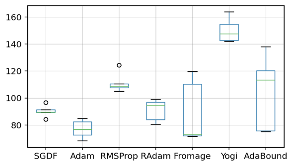

We evaluated the Wasserstein-GAN with gradient penalty (WGAN-GP) [47]. Using well-known optimizers [4, 61], the model was trained for 100 epochs. We then calculated the Frechet Inception Distance (FID) [24] which is a metric that measures the similarity between the real image and the generated image distribution and is used to assess the quality of the generated model (lower FID indicates superior performance). Five random runs were conducted, and the outcomes are presented in Figure 3. Results for SGD and MSVAG were extracted from Zhuang et al. [66].
Experimental results demonstrate that SGDF significantly enhances WGAN-GP model training, achieving a FID score higher than vanilla SGD and outperforming most adaptive optimization methods. The integration of a Wiener filter in SGDF facilitates smooth gradient updates, mitigating training oscillations and effectively addressing the issue of pattern collapse.
4.2 Top Eigenvalues of Hessian and Hessian Trace
The success of optimization algorithms in deep learning not only depends on their ability to minimize training loss but also critically hinges on the nature of the solutions they converge to. Adam-type algorithms tend to converge to sharp minima, characterized by large eigenvalues of the Hessian matrix [6].
We computed the Hessian spectrum of ResNet-18 trained on the CIFAR-100 dataset for 200 epochs using four optimization methods: SGD, SGDM, Adam, and SGDF. These experiments ensure that all methods achieve similar results on the training set. We employed power iteration [58] to compute the top eigenvalues of Hessian and Hutchinson’s method [59] to compute the Hessian trace. Histograms illustrating the distribution of the top 50 Hessian eigenvalues for each optimization method are presented in Fig. 4.
4.3 Visualization of Landscapes
We visualized the loss landscapes of models trained with SGD, SGDM, SGDF, and Adam using the ResNet-18 model on CIFAR-100, following the method in [34]. All models are trained with the same hyperparameters for 200 epochs, as detailed in Section 4.1. As shown in Fig. 5, SGDF finds flatter minima. Notably, the visualization reveals that Adam is more prone to converge to sharper minima.
4.4 Wiener Filter combines Adam
We’ve conducted comparative experiments on the CIFAR-100 dataset, evaluating both the vanilla Adam algorithm and Wiener Adam, which substitutes the first-moment gradient estimates in the Adam optimizer with Wiener filter estimates. The results are presented in Tab. 4, and the detailed test curves are depicted in Fig. 10. This suggests that our first-moment filter estimation method has the potential to be applied to other optimization methods.
| Model | VGG11 | ResNet34 | DenseNet121 |
|---|---|---|---|
| Wiener-Adam | 62.64 | 73.98 | 74.89 |
| Vanilla-Adam | 56.73 | 72.34 | 74.89 |
The performance improvement observed when using filter estimate can be attributed to several factors related to the nature of the Wiener filter and the architecture of the neural networks used.
Noise Reduction. The Wiener Filter is fundamentally designed to minimize the mean square error in the presence of noise. In the context of gradient estimation, this means it can effectively reduce the noise in the gradient updates. The vanilla Adam optimizer calculates the first moment (the mean) of the gradients, which may still include some noise components. By employing the Wiener filter, the algorithm may benefit from cleaner and more reliable gradient signals, thus improving the optimizer’s ability to converge to better minima.
Network Architecture. The impact of the Wiener Filter on gradient estimation varies with the network architecture’s unique handling of features and gradients. For VGG, which lacks residual connections, the Wiener filter significantly enhances performance by providing more accurate gradient estimations, reducing noise-induced errors, and leading to better overall accuracy. In contrast, the benefits are less pronounced in ResNet and DenseNet, which incorporate residual and dense connections, respectively. These architectures naturally promote more stable gradient flows through direct paths or dense layer interconnectivity, diminishing the additional advantage offered by the Wiener filter. Intuitively, we can find the loss landscape with residual connected networks in [34]. Thus, while the Wiener filter improves performance in simpler architectures like VGG, its impact is mitigated in more complex architectures where inherent features already assist in gradient stability.
5 Limitations
Theoretical Limitations. Our analysis relies on the common L-smooth condition for optimization continuity. Zhang et al. [64] propose gradient clipping, weakening this constraint. This suggests considering additional conditions for better understanding optimization in non-convex settings [52].
Empirical Limitations. Modern Large Language Models (LLMs) prioritize performance on training datasets [10, 36]. Discussing the theoretical properties of the Hessian matrix may lack relevance without comparable training losses. In practice, metrics like convergence speed and final loss values matter most.
6 Conclusion
In this paper, we introduce SGDF, a novel optimization method that estimates the gradient for faster convergence by leveraging both the variance of historical gradients and the current gradient. We demonstrate that SGDF yields solutions with a flat spectrum akin to SGD through Hessian spectral analysis. Through extensive experiments employing various deep learning architectures on benchmark datasets, we showcase SGDF’s superior performance compared to other state-of-the-art optimizers, striking a balance between convergence speed and generalization.
Acknowledgement
Zhipeng Yao thanks to Aram Davtyan and Prof. Dr. Paolo Favaro in the Computer Vision Group at the University of Bern for discussing and improving the paper.
Thanks to computational support from the Ascend AI Eco-Innovation Centre at the Shenyang AI Computing Hub.
References
- Arjovsky et al. [2017] Arjovsky, M., Chintala, S., and Bottou, L. Wasserstein gan. 2017.
- Balles & Hennig [2018] Balles, L. and Hennig, P. Dissecting adam: The sign, magnitude and variance of stochastic gradients. In International Conference on Machine Learning, pp. 404–413. PMLR, 2018.
- Bengio & Lecun [2007] Bengio, Y. and Lecun, Y. Scaling learning algorithms towards ai. 2007.
- Bernstein et al. [2020] Bernstein, J., Vahdat, A., Yue, Y., and Liu, M.-Y. On the distance between two neural networks and the stability of learning. Advances in Neural Information Processing Systems, 33:21370–21381, 2020.
- Bottou et al. [2018] Bottou, L., Curtis, F. E., and Nocedal, J. Optimization methods for large-scale machine learning. SIAM review, 60(2):223–311, 2018.
- Caldarola et al. [2022] Caldarola, D., Caputo, B., and Ciccone, M. Improving generalization in federated learning by seeking flat minima. ArXiv, 2022.
- Chandramoorthy et al. [2022] Chandramoorthy, N., Loukas, A., Gatmiry, K., and Jegelka, S. On the generalization of learning algorithms that do not converge. Advances in Neural Information Processing Systems, 35:34241–34257, 2022.
- Chen et al. [2018a] Chen, J., Zhou, D., Tang, Y., Yang, Z., Cao, Y., and Gu, Q. Closing the generalization gap of adaptive gradient methods in training deep neural networks. arXiv preprint arXiv:1806.06763, 2018a.
- Chen et al. [2018b] Chen, X., Liu, S., Sun, R., and Hong, M. On the convergence of a class of adam-type algorithms for non-convex optimization. arXiv preprint arXiv:1808.02941, 2018b.
- Chen et al. [2023] Chen, X., Liang, C., Huang, D., Real, E., Wang, K., Liu, Y., Pham, H., Dong, X., Luong, T., Hsieh, C.-J., et al. Symbolic discovery of optimization algorithms. arXiv preprint arXiv:2302.06675, 2023.
- Dauphin et al. [2014] Dauphin, Y., Pascanu, R., Gulcehre, C., Cho, K., Ganguli, S., and Bengio, Y. Identifying and attacking the saddle point problem in high-dimensional non-convex optimization. MIT Press, 2014.
- Davtyan et al. [2022] Davtyan, A., Sameni, S., Cerkezi, L., Meishvili, G., Bielski, A., and Favaro, P. Koala: A kalman optimization algorithm with loss adaptivity. In Proceedings of the AAAI Conference on Artificial Intelligence, volume 36, pp. 6471–6479, 2022.
- Defazio et al. [2014] Defazio, A., Bach, F., and Lacoste-Julien, S. Saga: A fast incremental gradient method with support for non-strongly convex composite objectives. In Advances in Neural Information Processing Systems, pp. 1646–1654, 2014.
- Deng et al. [2009] Deng, J., Dong, W., Socher, R., Li, L.-J., Li, K., and Fei-Fei, L. Imagenet: A large-scale hierarchical image database. In IEEE Conference on Computer Vision and Pattern Recognition, 2009.
- Dozat [2016] Dozat, T. Incorporating nesterov momentum into adam. ICLR Workshop, 2016.
- Du & Lee [2018] Du, S. S. and Lee, J. D. On the power of over-parametrization in neural networks with quadratic activation. 2018.
- Duchi et al. [2011] Duchi, John, Hazan, Elad, Singer, and Yoram. Adaptive subgradient methods for online learning and stochastic optimization. Journal of Machine Learning Research, 2011.
- Everingham et al. [2010] Everingham, M., Van Gool, L., Williams, C. K., Winn, J., and Zisserman, A. The pascal visual object classes (voc) challenge. International journal of computer vision, 88(2):303–338, 2010.
- Foret et al. [2021] Foret, P. et al. Sharpness-aware minimization for efficiently improving generalization. In ICLR, 2021. spotlight.
- Geman et al. [2014] Geman, S., Bienenstock, E., and Doursat, R. Neural networks and the bias/variance dilemma. Neural Computation, 4(1):1–58, 2014.
- Goodfellow et al. [2016] Goodfellow, I., Bengio, Y., and Courville, A. Deep learning. MIT Press, 2016.
- Hardt et al. [2015] Hardt, M., Recht, B., and Singer, Y. Train faster, generalize better: Stability of stochastic gradient descent. Mathematics, 2015.
- He et al. [2016] He, K., Zhang, X., Ren, S., and Sun, J. Deep residual learning for image recognition. In Proceedings of the IEEE conference on computer vision and pattern recognition, pp. 770–778, 2016.
- Heusel et al. [2017] Heusel, M., Ramsauer, H., Unterthiner, T., Nessler, B., Klambauer, G., and Hochreiter, S. Gans trained by a two time-scale update rule converge to a nash equilibrium. 2017.
- Hinton et al. [2012] Hinton, G., Srivastava, N., and Swersky, K. Neural networks for machine learning lecture 6a overview of mini-batch gradient descent. Cited on, 14(8):2, 2012.
- Huang et al. [2017] Huang, G., Liu, Z., Van Der Maaten, L., and Weinberger, K. Q. Densely connected convolutional networks. In Proceedings of the IEEE conference on computer vision and pattern recognition, pp. 4700–4708, 2017.
- Johnson & Zhang [2013] Johnson, R. and Zhang, T. Accelerating stochastic gradient descent using predictive variance reduction. Advances in neural information processing systems, 26, 2013.
- Kalman [1960] Kalman, R. E. A new approach to linear filtering and prediction problems. Journal of Basic Engineering, 1960.
- Kay [1993] Kay, S. M. Fundamentals of Statistical Signal Processing: Estimation Theory, volume 1. Prentice-Hall, Inc., 1993.
- Keskar et al. [2016] Keskar, N. S., Mudigere, D., Nocedal, J., Smelyanskiy, M., and Tang, P. T. P. On large-batch training for deep learning: Generalization gap and sharp minima. 2016.
- Keskar et al. [2017] Keskar, N. S. et al. On large-batch training for deep learning: Generalization gap and sharp minima. In ICLR, 2017.
- Kingma & Ba [2014] Kingma, D. P. and Ba, J. Adam: A method for stochastic optimization. arXiv preprint arXiv:1412.6980, 2014.
- Krizhevsky et al. [2009] Krizhevsky, A., Hinton, G., et al. Learning multiple layers of features from tiny images. 2009.
- Li et al. [2018] Li, H., Xu, Z., Taylor, G., Studer, C., and Goldstein, T. Visualizing the loss landscape of neural nets. Advances in neural information processing systems, 31, 2018.
- Lin et al. [2014] Lin, T.-Y., Maire, M., Belongie, S., Hays, J., Perona, P., Ramanan, D., Dollár, P., and Zitnick, C. L. Microsoft coco: Common objects in context. European Conference on Computer Vision (ECCV), 2014.
- Liu et al. [2023] Liu, H., Li, Z., Hall, D., Liang, P., and Ma, T. Sophia: A scalable stochastic second-order optimizer for language model pre-training. arXiv preprint arXiv:2305.14342, 2023.
- Liu et al. [2019] Liu, L., Jiang, H., He, P., Chen, W., Liu, X., Gao, J., and Han, J. On the variance of the adaptive learning rate and beyond. arXiv preprint arXiv:1908.03265, 2019.
- Loshchilov & Hutter [2017] Loshchilov, I. and Hutter, F. Decoupled weight decay regularization. arXiv preprint arXiv:1711.05101, 2017.
- Lucchi et al. [2022] Lucchi, A., Proske, F., Orvieto, A., Bach, F., and Kersting, H. On the theoretical properties of noise correlation in stochastic optimization. Advances in Neural Information Processing Systems, 35:14261–14273, 2022.
- Luo et al. [2019] Luo, L., Xiong, Y., Liu, Y., and Sun, X. Adaptive gradient methods with dynamic bound of learning rate. arXiv preprint arXiv:1902.09843, 2019.
- Monro [1951] Monro, R. S. a stochastic approximation method. Annals of Mathematical Statistics, 22(3):400–407, 1951.
- Ollivier [2019] Ollivier, Y. The extended kalman filter is a natural gradient descent in trajectory space. arXiv: Optimization and Control, 2019.
- Rao [1992] Rao, C. R. Information and the accuracy attainable in the estimation of statistical parameters. In Breakthroughs in Statistics: Foundations and basic theory, pp. 235–247. Springer, 1992.
- Reddi et al. [2019] Reddi, S. J., Kale, S., and Kumar, S. On the convergence of adam and beyond. 2019.
- Ren et al. [2015] Ren, S., He, K., Girshick, R., and Sun, J. Faster r-cnn: Towards real-time object detection with region proposal networks. Neural Information Processing Systems (NIPS), 2015.
- Ruder [2016] Ruder, S. An overview of gradient descent optimization algorithms. 2016.
- Salimans et al. [2016] Salimans, T., Goodfellow, I., Zaremba, W., Cheung, V., Radford, A., and Chen, X. Improved techniques for training gans. Advances in neural information processing systems, 29, 2016.
- Schmidt et al. [2017] Schmidt, M., Roux, N. L., and Bach, F. Minimizing finite sums with the stochastic average gradient. Mathematical Programming, 162(1):83–112, 2017.
- Simonyan & Zisserman [2014] Simonyan, K. and Zisserman, A. Very deep convolutional networks for large-scale image recognition. Computer Science, 2014.
- Sutskever et al. [2013] Sutskever, I., Martens, J., Dahl, G., and Hinton, G. On the importance of initialization and momentum in deep learning. In International conference on machine learning, pp. 1139–1147. PMLR, 2013.
- Vuckovic [2018] Vuckovic, J. Kalman gradient descent: Adaptive variance reduction in stochastic optimization. ArXiv, 2018.
- Wang et al. [2022] Wang, B., Zhang, Y., Zhang, H., Meng, Q., Ma, Z.-M., Liu, T.-Y., and Chen, W. Provable adaptivity in adam. arXiv preprint arXiv:2208.09900, 2022.
- Wiener [1950] Wiener, N. The extrapolation, interpolation and smoothing of stationary time series, with engineering applications. Journal of the Royal Statistical Society Series A (General), 1950.
- Wilson et al. [2017] Wilson, A. C., Roelofs, R., Stern, M., Srebro, N., and Recht, B. The marginal value of adaptive gradient methods in machine learning. 2017.
- Xie et al. [2020] Xie, Z., Wang, X., Zhang, H., Sato, I., and Sugiyama, M. Adai: Separating the effects of adaptive learning rate and momentum inertia. arXiv preprint arXiv:2006.15815, 2020.
- Xie et al. [2022] Xie, Z., Tang, Q. Y., Cai, Y., Sun, M., and Li, P. On the power-law spectrum in deep learning: A bridge to protein science. 2022.
- Yang et al. [2023] Yang, N., Tang, C., and Tu, Y. Stochastic gradient descent introduces an effective landscape-dependent regularization favoring flat solutions. Physical Review Letters, 130(23):237101, 2023.
- Yao et al. [2018] Yao, Z., Gholami, A., Lei, Q., Keutzer, K., and Mahoney, M. W. Hessian-based analysis of large batch training and robustness to adversaries. 2018.
- Yao et al. [2020a] Yao, Z., Gholami, A., Keutzer, K., and Mahoney, M. W. Pyhessian: Neural networks through the lens of the hessian. In International Conference on Big Data, 2020a.
- Yao et al. [2020b] Yao, Z., Gholami, A., Shen, S., Keutzer, K., and Mahoney, M. W. Adahessian: An adaptive second order optimizer for machine learning. arXiv preprint arXiv:2006.00719, 2020b.
- Zaheer et al. [2018] Zaheer, M., Reddi, S., Sachan, D., Kale, S., and Kumar, S. Adaptive methods for nonconvex optimization. Advances in neural information processing systems, 31, 2018.
- Zeiler [2012] Zeiler, M. D. Adadelta: An adaptive learning rate method. arXiv e-prints, 2012.
- Zhang et al. [2016] Zhang, C., Bengio, S., Hardt, M., Recht, B., and Vinyals, O. Understanding deep learning requires rethinking generalization. 2016.
- Zhang et al. [2019] Zhang, J., He, T., Sra, S., and Jadbabaie, A. Why gradient clipping accelerates training: A theoretical justification for adaptivity. arXiv preprint arXiv:1905.11881, 2019.
- Zhang et al. [2023] Zhang, X., Xu, R., Yu, H., Zou, H., and Cui, P. Gradient norm aware minimization seeks first-order flatness and improves generalization. IEEE/CVF Conference on Computer Vision and Pattern Recognition (CVPR), 2023.
- Zhuang et al. [2020] Zhuang, J., Tang, T., Ding, Y., Tatikonda, S. C., Dvornek, N., Papademetris, X., and Duncan, J. Adabelief optimizer: Adapting stepsizes by the belief in observed gradients. Advances in neural information processing systems, 33:18795–18806, 2020.
Appendix A Method Derivation (Section 3 in main paper)
A.1 Wiener Filter Derivation for Gradient Estimation (Main paper Section 3.1)
Given the sequence of gradients in a stochastic gradient descent process, we aim to find an estimate that incorporates information from both the historical gradients and the current gradient. The Wiener Filter provides an estimate that minimizes the mean squared error. We begin by constructing the estimate as a simple average and then refine it using the properties of the Wiener Filter.
| (6) | ||||
In the above derivation, step (a) replaces the arithmetic mean of gradients with the momentum term . The Wiener gain is then introduced to update the gradient estimate with information from the new gradient.
By defining as the weighted combination of the momentum term and the current gradient , we can compute the variance of as follows:
| (7) | ||||
Minimizing the variance of with respect to , by setting the derivative , yields:
| (8) | ||||
The final expression for shows that the optimal interpolation coefficient is the ratio of the variance of the momentum term to the sum of the variances of the momentum term and the current gradient. This result exemplifies the essence of the Wiener Filter: optimally combining past information with new observations to reduce estimation error due to noisy data.
A.2 Variance Correction (Correction factor in main paper Section 3.1)
The momentum term is defined as:
| (9) |
which means that the momentum term is a weighted sum of past gradients, where the weights decrease exponentially over time.
To compute the variance of the momentum term , we first observe that since are independent and identically distributed with a constant variance , the variance of the momentum term can be obtained by summing up the variances of all the weighted gradients.
The variance of each weighted gradient is , because the variance operation has a quadratic nature, so the weight becomes in the variance computation.
Therefore, the variance of is the sum of all these weighted variances:
| (10) |
The factor comes from the multiplication factor in the momentum update formula, which is also squared when calculating the variance.
The summation part is a geometric series, which can be formulated as:
| (11) |
As , and given that , we note that , and the geometric series sum converges to:
| (12) |
Consequently, the long-term variance of the momentum term is expressed as:
| (13) |
This result shows how the effective gradient noise is reduced by the momentum term, which is a factor of compared to the variance of the gradients .
A.3 Fusion Gaussian distribution (Main paper Section 3.2)
Consider two Gaussian distributions for the momentum term and the current gradient :
-
•
The momentum term is normally distributed with mean and variance , denoted as .
-
•
The current gradient is normally distributed with mean and variance , denoted as .
The product of their probability density functions is given by:
| (14) |
The goal is to find equivalent mean and variance for the new Gaussian distribution that matches the product:
| (15) |
We derive the expression for combining these two distributions. For convenience, let us define the variable as follows:
| (16) | ||||
Through coefficient matching in the exponential terms, we obtain the new mean and variance:
| (17) |
The new mean is a weighted average of the two means, and , with weights inversely proportional to their variances. This places between and , closer to the mean with the smaller variance. The new standard deviation is smaller than either of the original standard deviations and , which reflects the reduced uncertainty in the estimate due to the combination of information from both sources. This is a direct consequence of the Wiener Filter’s optimality in the mean-square error sense.
A.4 Fokker Planck modelling (Theorem 3.1 in main paper)
Theorem A.1.
Consider a system described by the Fokker-Planck equation, evolving the probability density function in one-dimensional and multi-dimensional parameter spaces. Given a loss function , and the noise variance or diffusion matrix satisfying or , where is a positive lower bound constant, known as the Cramér-Rao lower bound. In the steady state condition, i.e., , the analytical form of the probability density can be obtained by solving the corresponding Fokker-Planck equation. These solutions reveal the probability distribution of the system at steady state, described as follows:
One-dimensional case In a one-dimensional parameter space, the probability density function is
| (18) |
where is a normalization constant, ensuring the total probability sums to one.
Multi-dimensional case In a multi-dimensional parameter space, the probability density function is
| (19) |
Here, is also a normalization constant, ensuring the total probability sums to one, assuming , where is the Kronecker delta.
Proof.
one-dimensional Fokker-Planck equation: Given the one-dimensional Fokker-Planck equation:
| (20) |
where is the loss function, and is the variance of the noise, with representing a positive lower bound for the variance. denotes the probability density of finding the state of the system near a given point or region
Derivation of the Steady-State Distribution:
In the steady state condition, , thus the equation simplifies to:
| (21) |
Our goal is to find the probability density as a function of .
By integrating, we obtain:
| (22) |
Next, we set as the probability current, and we have:
| (23) |
Upon integration, we get:
| (24) |
where is an integration constant. Assuming the probability current vanishes at infinity, then .
Therefore, we have:
| (25) |
This equation can be rewritten as:
| (26) |
Now, leveraging the variance lower bound , we analyze the above equation. Since is a positive constant, we can further integrate to get :
| (27) |
where is an integration constant.
Solving for , we get:
| (28) |
Since we know that has a lower bound, is bounded above, which suggests that will not explode at any specific value of .
multi-dimensional Fokker-Planck equation: Consider a multi-dimensional parameter space and a loss function . The evolution of the probability density function in this space governed by the Fokker-Planck equation is given by:
| (29) |
where are elements of the diffusion matrix, representing the intensity and correlation of the stochastic in the directions and . At the steady state, where the time derivative of vanishes, we find:
| (30) |
Assuming where is the Kronecker delta, and , the equation simplifies to:
| (31) |
Integrating with respect to , we obtain a set of equations:
| (32) |
where is an integration constant. Assuming , which corresponds to no flux at the boundaries, we can solve for :
| (33) |
where is a normalization constant ensuring that the total probability integrates to one.
Exploration Efficacy of SGD due to Variance Lower Bound The existence of a variance lower bound in Stochastic Gradient Descent (SGD) critically enhances the algorithm’s exploration capabilities, particularly in regions of the loss landscape where gradients are minimal. By preventing the probability density function from becoming unbounded, it ensures continuous exploration and increases the probability of converging to flat minima that are associated with better generalization properties. This principle holds true across both one-dimensional and multi-dimensional scenarios, making the variance lower bound an essential consideration for optimizing SGD’s performance in finding robust, generalizable solutions.
Appendix B Convergence analysis in convex online learning case (Theorem 3.2 in main paper).
Assumption B.1.
Variables are bounded: . Gradients are bounded: .
Definition B.2.
Let be the loss at time and be the loss of the best possible strategy at the same time. The cumulative regret at time is defined as:
| (34) |
Definition B.3.
If a function : is convex if for all for all ,
| (35) |
Also, notice that a convex function can be lower bounded by a hyperplane at its tangent.
Lemma B.4.
If a function is convex, then for all ,
| (36) |
The above lemma can be used to upper bound the regret, and our proof for the main theorem is constructed by substituting the hyperplane with SGDF update rules.
The following two lemmas are used to support our main theorem. We also use some definitions to simplify our notation, where and as the element. We denote as a vector that contains the dimension of the gradients over all iterations till
Lemma B.5.
Let and be defined as above and bounded,
| (37) |
Then,
| (38) |
Proof. We will prove the inequality using induction over . For the base case :
| (39) |
Assuming the inductive hypothesis holds for , for the inductive step:
| (40) | ||||
Given,
| (41) |
taking the square root of both sides, we get:
| (42) | ||||
Substituting into the previous inequality:
| (43) |
Lemma B.6.
Let bounded , , the following inequality holds
| (44) |
Proof. Under the inequality: . We can expand the last term in the summation using the updated rules in Algorithm 1,
| (45) | ||||
Similarly, we can upper-bound the rest of the terms in the summation.
| (46) | ||||
For , using the upper bound on the arithmetic-geometric series, :
| (47) |
Apply Lemma B.5,
| (48) |
Theorem B.7.
Assume that the function has bounded gradients, , for all and the distance between any generated by SGDF is bounded, , for any , and . Let . For all , SGDF achieves the following guarantee:
| (49) |
Proof of convex Convergence.
We aim to prove the convergence of the algorithm by showing that is bounded, or equivalently, that converges to zero as goes to infinity.
To express the cumulative regret in terms of each dimension, let and represent the loss and the best strategy’s loss for the th dimension, respectively. Define as:
| (50) |
Then, the overall regret can be expressed in terms of all dimensions as:
| (51) |
Establishing the Connection: From the Iteration of to
Using Lemma B.4, we have,
| (52) |
From the update rules presented in algorithm 1,
| (53) | ||||
We focus on the dimension of the parameter vector . Subtract the scalar and square both sides of the above update rule, we have,
| (54) |
Separating items:
| (55) |
We then deal with (1), (2) and (3) separately.
For the first term (1), we have:
| (56) | ||||
Given that and , we can bound it as:
| (57) | ||||
For the second term (2), we have:
| (58) | ||||
For the third term (3), we have:
| (59) | ||||
Collate all the items that we have:
| (60) |
Appendix C Convergence analysis for non-convex stochastic optimization (Theorem 3.3 in main paper).
We have relaxed the assumption on the objective function, allowing it to be non-convex, and adjusted the criterion for convergence from the statistic to . Let’s briefly review the assumptions and the criterion for convergence after relaxing the assumption:
Assumption C.1.
-
•
A1 Bounded variables (same as convex). or for any dimension of the variable,
-
•
A2 The noisy gradient is unbiased. For , the random variable is defined as , satisfy , , and when , and are statistically independent, i.e., .
-
•
A3 Bounded gradient and noisy gradient. At step , the algorithm can access a bounded noisy gradient, and the true gradient is also bounded. .
-
•
A4 The property of function. The objective function is a global loss function, defined as . Although is no longer a convex function, it must still be a -smooth function, i.e., it satisfies (1) is differentiable, exists everywhere in the domain; (2) there exists such that for any and in the domain, (first definition)
(62) or (second definition)
(63) This condition is also known as L - Lipschitz.
Definition C.2.
The criterion for convergence is the statistic :
| (64) |
When , if the amortized value of , , we consider such an algorithm to be convergent, and generally, the slower grows with , the faster the algorithm converges.
Definition C.3.
Define as
| (65) |
Theorem C.4.
Consider a non-convex optimization problem. Suppose assumptions A1-A5 are satisfied, and let . For all , SGDF achieves the following guarantee:
| (66) |
where denotes the minimum of the squared-paradigm expectation of the gradient, is the learning rate at the -th step, are constants independent of and , is a constant independent of , and the expectation is taken w.r.t all randomness corresponding to .
Proof of convex Convergence.
Since is an L-smooth function,
| (67) |
Thus,
| (68) | ||||
Next, we will deal with the three terms (1), (2), and (3) separately.
For term (1)
When ,
When ,
| (69) | ||||
Where (a) holds because for any :
-
•
.
-
•
, or for any dimension of the variable :
For term (2)
When ,
| (70) | ||||
Thus,
| (71) | ||||
When ,
| (72) | ||||
Due to
| (73) | ||||
So,
| (74) | ||||
We have:
| (75) | ||||
Because
-
•
,
-
•
-
•
, we have
| (76) | ||||
| (77) |
Therefore
| (78) |
For term (3)
When , referring to the case of in the previous subsection,
| (79) | ||||
The last equality is due to the definition of : . Let’s consider them separately:
| (80) | ||||
| (81) | ||||
Thus
| (82) | ||||
When ,
| (83) | ||||
Start by looking at the first item after the equal sign:
| (84) | ||||
The second and third terms after the equal sign:
| (85) | ||||
The fourth and fifth terms after the equal sign:
| (86) | ||||
Final:
| (87) | ||||
Summarizing the results
Let’s start summarizing: when ,
| (88) |
Taking the expectation over the random distribution of on both sides of the inequality:
| (89) |
When ,
| (90) | ||||
Taking the expectation over the random distribution of on both sides of the inequality:
| (91) | ||||
Since the value of is independent of , they are statistically independent of :
| (92) | ||||
Summing up both sides of the inequality for :
• Left side of the inequality (can be reduced to maintain the inequality)
| (93) | ||||
Since , , and both are deterministic:
| (94) | ||||
• The right side of the inequality (can be enlarged to keep the inequality valid)
We perform a series of substitutions to simplify the symbols:
When ,
-
1.
-
2.
-
3.
-
4.
-
5.
-
6.
When ,
-
1.
-
2.
-
3.
After substitution,
| (95) | ||||
Combining the results of scaling on both sides of the inequality:
| (96) | ||||
Due to ,
| (97) | ||||
Then let , , therefore
| (98) | ||||
Since , we have:
| (99) |
Appendix D Detailed Experimental Supplement
We performed extensive comparisons with other optimizers, including SGD [41], Adam[32], RAdam[37] and AdamW[38]. The experiments include: (a) image classification on CIFAR dataset[33] with VGG [49], ResNet [23] and DenseNet [26], and image recognition with ResNet on ImageNet [14].
D.1 Image classification with CNNs on CIFAR
For all experiments, the model is trained for 200 epochs with a batch size of 128, and the learning rate is multiplied by 0.1 at epoch 150. We performed extensive hyperparameter search as described in the main paper. Detailed experimental parameters we place in Tab. 5. Here we report both training and test accuracy in Fig. 6 and Fig. 7. SGDF not only achieves the highest test accuracy, but also a smaller gap between training and test accuracy compared with other optimizers.
| Optimizer | Learning Rate | Epochs | Schedule | Weight Decay | Batch Size | |||
|---|---|---|---|---|---|---|---|---|
| SGDF | 0.3 | 0.9 | 0.999 | 200 | StepLR | 0.0005 | 128 | 1e-8 |
| SGD | 0.1 | 0.9 | - | 200 | StepLR | 0.0005 | 128 | - |
| Adam | 0.001 | 0.9 | 0.999 | 200 | StepLR | 0.0005 | 128 | 1e-8 |
| RAdam | 0.001 | 0.9 | 0.999 | 200 | StepLR | 0.0005 | 128 | 1e-8 |
| AdamW | 0.001 | 0.9 | 0.999 | 200 | StepLR | 0.01 | 128 | 1e-8 |
| MSVAG | 0.1 | 0.9 | 0.999 | 200 | StepLR | 0.0005 | 128 | 1e-8 |
| AdaBound | 0.001 | 0.9 | 0.999 | 200 | StepLR | 0.0005 | 128 | - |
| Sophia | 0.0001 | 0.965 | 0.99 | 200 | StepLR | 0.1 | 128 | - |
| Lion | 0.00002 | 0.9 | 0.99 | 200 | StepLR | 0.1 | 128 | - |
Note: StepLR indicates a learning rate decay by a factor of 0.1 at the 150th epoch.
D.2 Image Classification on ImageNet
We experimented with a ResNet18 on ImageNet classification task. For SGD, we set an initial learning rate of 0.1, and multiplied by 0.1 every 30 epochs; for SGDF, we use an initial learning rate of 0.5, set = 0.5. Weight decay is set as for both cases. To match the settings in [37]. Detailed experimental parameters we place in Tab. 6. As shown in Fig. 8, SGDF achieves an accuracy very close to SGD.
| Optimizer | Learning Rate | Epochs | Schedule | Weight Decay | Batch Size | |||
|---|---|---|---|---|---|---|---|---|
| SGDF | 0.5 | 0.5 | 0.999 | 100 | StepLR | 0.0005 | 256 | 1e-8 |
| SGD | 0.1 | - | - | 100 | StepLR | 0.0005 | 256 | - |
| SGDF | 0.5 | 0.5 | 0.999 | 90 | Cosine | 0.0005 | 256 | 1e-8 |
| SGD | 0.1 | - | - | 90 | Cosine | 0.0005 | 256 | - |
Note: StepLR indicates a learning rate decay by a factor of 0.1 every 30 epochs.
D.3 Objective Detection on PASCAL VOC
We show the results on PASCAL VOC[18]. Object detection with a Faster-RCNN model[45]. Detailed experimental parameters we place in Tab. 7. The results are reported in Tab. 2, and detection examples shown in Fig. 9. These results also illustrate that our method is still efficient in object detection tasks.
| Optimizer | Learning Rate | Epochs | Schedule | Weight Decay | Batch Size | |||
|---|---|---|---|---|---|---|---|---|
| SGDF | 0.01 | 0.9 | 0.999 | 4 | StepLR | 0.0001 | 2 | 1e-8 |
| SGD | 0.01 | 0.9 | - | 4 | StepLR | 0.0001 | 2 | - |
| Adam | 0.0001 | 0.9 | 0.999 | 4 | StepLR | 0.0001 | 2 | 1e-8 |
| AdamW | 0.0001 | 0.9 | 0.999 | 4 | StepLR | 0.0001 | 2 | 1e-8 |
| RAdam | 0.0001 | 0.9 | 0.999 | 4 | StepLR | 0.0001 | 2 | 1e-8 |
Note: StepLR schedule indicates a learning rate decay by a factor of 0.1 at the last epoch.
D.4 Image Generation.
We experiment with one of the most widely used models, the Wasserstein-GAN with gradient penalty (WGAN-GP)[47] using a small model with a vanilla CNN generator. Using popular optimizer[40, 61, 2, 4], we train the model for 100 epochs, generate 64,000 fake images from noise, and compute the Frechet Inception Distance (FID)[24] between the fake images and real dataset (60,000 real images). FID score captures both the quality and diversity of generated images and is widely used to assess generative models (lower FID is better). For SGD and MSVAG, we report results from [66]. We perform 5 runs of experiments, and report the results in Fig. 5. Detailed experimental parameters we place in Tab. 8.
| Optimizer | Learning Rate | Epochs | Batch Size | |||
|---|---|---|---|---|---|---|
| SGDF | 0.01 | 0.5 | 0.999 | 100 | 64 | 1e-8 |
| Adam | 0.0002 | 0.5 | 0.999 | 100 | 64 | 1e-8 |
| AdamW | 0.0002 | 0.5 | 0.999 | 100 | 64 | 1e-8 |
| Fromage | 0.01 | 0.5 | 0.999 | 100 | 64 | 1e-8 |
| RMSProp | 0.0002 | 0.5 | 0.999 | 100 | 64 | 1e-8 |
| AdaBound | 0.0002 | 0.5 | 0.999 | 100 | 64 | 1e-8 |
| Yogi | 0.01 | 0.9 | 0.999 | 100 | 64 | 1e-8 |
| RAdam | 0.0002 | 0.5 | 0.999 | 100 | 64 | 1e-8 |
D.5 Extended Experiment.
The study involves evaluating the vanilla Adam optimization algorithm and its enhancement with a Wiener filter on the CIFAR-100 dataset. Fig. 9 contains detailed test accuracy curves for both methods across different models. The results indicate that the adaptive learning rate algorithms exhibit improved performance when supplemented with the proposed first-moment filter estimation. This suggests that integrating a Wiener filter with the Adam optimizer may improve performance.
D.6 Optimizer Test.
We derived a correction factor from the geometric progression to correct the variance of by the correction factor. So we test the SGDF with or without correction in VGG, ResNet, DenseNet on CIFAR. We report both test accuracy in Fig. 11. It can be seen that the SGDF with correction exceeds the uncorrected one.
We built a simple neural network to test the convergence speed of SGDF compared to SGDM and vanilla SGD. We trained 5 epochs and recorded the loss every 30 iterations. As Fig. 12 shown, the convergence rate of the filter method surpasses that of the momentum method, which in turn exceeds that of vanilla SGD.


![[Uncaptioned image]](https://cdn.awesomepapers.org/papers/921e89db-7462-418b-9285-b0c558cd99ae/sgdf_test1_result.png)
![[Uncaptioned image]](https://cdn.awesomepapers.org/papers/921e89db-7462-418b-9285-b0c558cd99ae/sgdm_test1_result.png)
![[Uncaptioned image]](https://cdn.awesomepapers.org/papers/921e89db-7462-418b-9285-b0c558cd99ae/adam_test1_result.png)
![[Uncaptioned image]](https://cdn.awesomepapers.org/papers/921e89db-7462-418b-9285-b0c558cd99ae/adamw_test1_result.png)
![[Uncaptioned image]](https://cdn.awesomepapers.org/papers/921e89db-7462-418b-9285-b0c558cd99ae/radam_test1_result.png)
