Shortcuts to Adiabaticity in Digitized Adiabatic Quantum Computing
Abstract
Shortcuts to adiabaticity are well-known methods for controlling the quantum dynamics beyond the adiabatic criteria, where counter-diabatic (CD) driving provides a promising means to speed up quantum many-body systems. In this work, we show the applicability of CD driving to enhance the digitized adiabatic quantum computing paradigm in terms of fidelity and total simulation time. We study the state evolution of an Ising spin chain using the digitized version of the standard CD driving and its variants derived from the variational approach. We apply this technique in the preparation of Bell and Greenberger-Horne-Zeilinger states with high fidelity using a very shallow quantum circuit. We implement this proposal in the IBM quantum computer, proving its usefulness for the speed up of adiabatic quantum computing in noisy intermediate-scale quantum devices.
I introduction
Quantum computing is known to have significant advantages in solving certain computational tasks, such as simulating quantum systems Feynman (1999); Georgescu et al. (2014); Houck et al. (2012); Lanyon et al. (2011); Gerritsma et al. (2010), machine learning Biamonte et al. (2017); Lloyd et al. (2013); Dunjko et al. (2016); Schuld and Killoran (2019), solving optimization problems Moll et al. (2018); Farhi and Harrow (2016); Arute et al. (2020), cryptography Gisin et al. (2002); Bennett and Brassard (2014), and several others. Recent advancements in quantum technologies have already shown that quantum computers can outperform currently existing classical computers Arute et al. (2019).
Quantum adiabatic algorithms (QAA) Farhi et al. (2001); Ambainis and Regev (2004); Young et al. (2010); Peng et al. (2008) are one of the leading candidates for solving optimization problems Reichardt (2004); Steffen et al. (2003); Bapst et al. (2013). In adiabatic quantum computation (AdQC), we start with a simple Hamiltonian whose ground state can be easily prepared and evolve the system adiabatically to the ground state of the final Hamiltonian, which encodes the solution of the optimization problem. This is embodied by the well-known method of quantum annealing Das and Chakrabarti (2008). Quantum annealers, such as the D-Wave machine Johnson et al. (2011), provide the test-bed for adiabatic algorithms Boixo et al. (2013). Despite its applications, quantum annealers have certain limitations, such as difficulty in implementing non-stoquastic Hamiltonian, limited qubit connectivity and noise. Although AdQC is equivalent to the standard circuit model Aharonov et al. (2008), the advantage of digital quantum computation (DQC) over quantum annealers is that the circuit model offers more flexibility to construct arbitrary interactions, and it is consistent with error correction. The recent work by R. Barends et al. Barends et al. (2016) combines the advantage of AdQC and the circuit model, termed as digitized adiabatic quantum computation (DAdQC), has been presented and implemented on a superconducting system.
QAAs are generally governed by the quantum adiabatic theorem that restricts a system to evolve along a specific eigenstate, i.e., from the ground state of an initial Hamiltonian to the ground state of a final Hamiltonian , while the evolution is considerably slow. The computation time for the QAA depends on the minimum energy gap between the successive eigenstates during the evolution. When the system size increases, this poses a significant disadvantage for the implementation of QAA as the energy gap decreases with increasing system size, which ends up in transition between various instantaneous eigenstates. One has to increase the adiabatic evolution time to circumvent such an issue. However, in practice, evolution time for QAA is significantly larger than the coherence time of the current quantum computers, leading to the loss of fidelity of the evolution.
The techniques of “Shortcut to adiabaticity” (STA) Torrontegui et al. (2013); Guéry-Odelin et al. (2019) have been developed during the past decade and proved to be extremely useful for accelerating quantum adiabatic processes in general Takahashi (2019). Various techniques like counter diabatic (CD) driving (equivalently transitionless quantum algorithm) Demirplak and Rice (2003, 2005); Berry (2009), invariant based inverse engineering Chen et al. (2010, 2011), fast-forward approach Masuda and Nakamura (2008, 2010) are rigorously explored and implemented in several studies Schaff et al. (2010); An et al. (2016); Du et al. (2016). Among these works, studies related to quantum spin systems such as Ising and Heisenberg spin models are of particular interest due to their relevance to the applicability and ease of implementation in the development of modern-day quantum algorithms Lucas (2014). In particular, the CD driving has been useful for studying fast dynamics del Campo et al. (2012); Özgüler et al. (2018); Takahashi (2013); Hartmann and Lechner (2019); Petiziol et al. (2018), preparation of entangled states Opatrnỳ and Mølmer (2014); Petiziol et al. (2019); Ji et al. (2019); Zhou et al. (2020), quantum annealing Vinci and Lidar (2017); Takahashi (2017); Passarelli et al. (2020) and, others.
In this work, we explore the STA techniques to enhance the performance of the DAdQC using Ising spin systems. Starting from a single spin, we extend our study to many spins with nearest-neighbor interactions using the CD driving. We find out that the CD interactions in the QAA improve the fidelity remarkably compared to the previous studies. Due to the difficulty in the implementation of the exact CD term for a many-body system, we opt to find local CD terms that can drive smaller systems precisely and able to achieve the target state in very few time steps. By considering approximate CD terms using the nested commutator, we study the non-integrable Ising-model and extend this idea for the preparation of Bell state and GHZ state in larger systems.
The paper is organized as follows. In the next Sec. II, we give a detailed insight into the implementation of STA in a single spin, where the CD interaction can be exactly calculated using Berry’s formula. Sec. III explains the application of the approximate local CD driving and its limitations when applied to strongly interacting many-spin systems. In Sec. IV, we show the improvement in fidelity when the approximate CD driving is calculated using the nested commutator through the adiabatic gauge potential using the variational approach. This is followed by an example of entangled state preparation, where we show the preparation of Bell state and GHZ state for few spin systems with high fidelity. In the final Sec. V, we summarize our findings and discuss the scope for future research.
II Single spin system
We begin our heuristic discussions with a single spin in the presence of time-dependent external magnetic-field , represented by a two-level Hamiltonian, given by
| (1) |
where represents the Pauli matrices, and the superscript represents the number of spin. Following the general method for AdQC, also that of quantum annealing, we express this Hamiltonian as a combination of two time-independent parts.
| (2) |
and are time-independent with ground states and , respectively. The time dependence of the system is introduced through the parameter . The initial Hamiltonian is chosen as , and the final Hamiltonian as , where and being the magnetic field strength along respective directions. Such a choice leads to express the magnetic field effectively as . AdQC, in its rudimentary approach, allows to be any function that varies from to and drives the system from to . Although, the most general way to choose it as a linear function, here to begin with, it is considered as , where with being the total evolution time. Although is extremely elementary and can easily be implemented in the circuit model Sieberer et al. (2019), there are hints that the evolution can be improved significantly using the STA Özgüler et al. (2018). In this case, one should be tempted to find out the CD term, which is somewhat straightforward to calculate using Berry (2009),
| (3) |
yielding the explicit form as following,
| (4) |
Therefore, the total Hamiltonian assisted with CD term becomes
| (5) |
Note that the introduction of the CD term should not affect the initial and final states, since should always satisfy the boundary conditions, . Also, the STA methods generally follow the inverse engineering approach of quantum control, i.e., designing the interaction for achieving the desired eigenstates. Therefore the notion of the eigenstate, although not that essential in traditional AdQC, turns out to be extremely important in the present case. Here, the initial state of is chosen in the computational basis, i.e., , as and the final state is, . It should be noted that and are the natural ground states of and , respectively, but these choices are not restricted to the ground states only. However, such a choice restraints the qubit in the ground state, minimizing the effect of the decoherences.
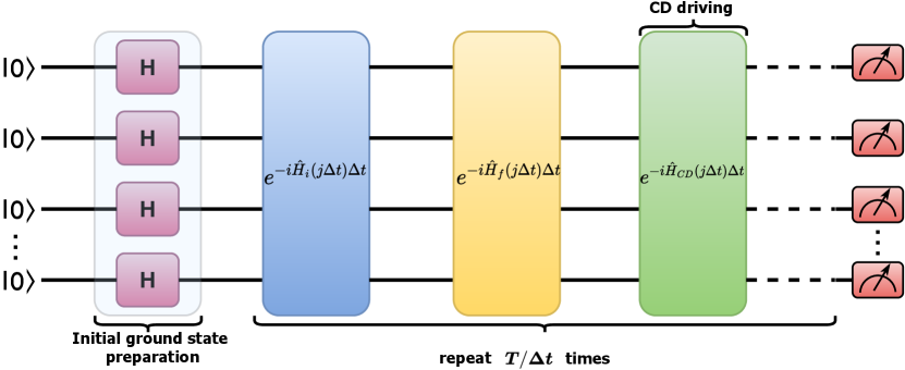
To implement the evolution using one qubit, we used first-order Trotter-Suzuki formula. The time evolution is digitized with number of small time steps (see Eq (18)). Ideally, the discretized version of AdQC approaches the actual adiabatic evolution for , (). Although, in real situations, is finite and it has to be a relatively small number since each trotter step is being implemented by three rotation gates (see Appendix A). The error associated with the first-order trotterization is Suzuki (1976).
To perform the simulation, we used publicly available five qubit superconducting quantum computer of IBM Quantum Experience ibm . For the single spin experiment we use qubit on . Since the single qubit gate error of the device is of the order of , the initial state is prepared with very high fidelity. Also a significant error in this simulation comes from the readout error , for that we used the error mitigation technique using matrix inversion method described in Appendix C.
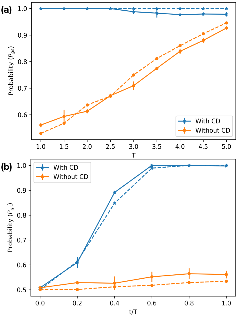
In the simulation, time evolution takes place between to and measured in the computational basis, which restricts the variation of the probability between to , see Fig. 2. Since the trotter error is of the order , we choose, , and for the comparison of the evolution using DAdQC and STA assisted DAdQC. To study the probability of final ground state , where denotes the time evolved state of , measurement is performed at each progressing time step. Fig. 2(b) shows a single evolution of the qubit governed by both Eq. (2) and Eq. (5), using both simulation and experiment on a real quantum device. With the application of CD driving , the probability of getting the state from the experiment comes out to be around . Whereas, when the CD driving is zero, i.e., for the adiabatic evolution, the final state probability is around only. However, if the evolution is extended for a larger , we could obtain a much higher probability, even without , a signature of the typical adiabatic process. This is evident in Fig. 2(a), where the fidelity of the evolution (in the computational basis) for different is shown. Even when () using the STA method, the final ground state is reached with nearly unit fidelity. We observe that fidelity for the STA method for large maintains its value at around . However, for the adiabatic case, fidelity gradually increases with increasing simulation time and the average fidelity will be around for . Notice that in Fig. 2(a), the experimental values differ slightly from the exact simulation values, and the difference is slightly larger for the STA assisted case. As increases, the circuit depth becomes larger, which results in ramping up the gate errors, affecting STA more than the adiabatic case as it requires more gates for implementation.
III LOCAL COUNTER-DIABATIC DRIVING
The results in Sec. II establishes the fact that STA assisted DAdQC shows significant improvement over the DAdQC, at least when a single qubit is considered. However, such implementation becomes far more interesting when multiple qubits are considered. The simplest choice is a system of interacting spins in one-dimensional lattice, coupled by a time-dependent exchange interaction with a rotating magnetic field is acting upon it. Here we consider to constitute type interaction with being the coupling amplitude. The spins are initially aligned along the transverse magnetic field, , while an Ising Hamiltonian represents the system’s final state. The total Hamiltonian is represented as,
| (6) |
The scheduling is chosen similarly, as in Eq. (2). The traditional approaches to finding the CD driving are predominantly limited to two and three-level systems and become more complex for higher dimensional many-body systems. However, for interacting many spin systems, as in the preceding section, a local CD driving could be more useful. Instead of acting on the whole system, a set of approximated interactions could be designed to control the spins individually. Such type of local CD driving is more general and can be extended to a larger number of spins.
III.0.1 Local CD from Berry’s algorithm
To realize such CD driving, it is intuitive to approximate the system to a non-interacting one. Using mean-field approximation, this can be achieved effectively for an infinite-range Ising model Hatomura (2017). However, this is problematic for DAdQC, as it requires self-consistent feedback after every step. Instead, we consider a more direct approach. Since, at , the spins have no mutual interaction and are dictated by the transverse magnetic field, it can be assumed that, during the evolution, the magnitude of and grows gradually from zero to some maximum value while the system evolves gradually from to . Therefore, we approximate that those spins are governed by a local effective magnetic field, given by , where . Subsequently, the local CD driving is calculated and summed over for each spin using Eq. (3),
| (7) |
Therefore, the modified Hamiltonian that governs the evolution can be expressed as
| (8) |
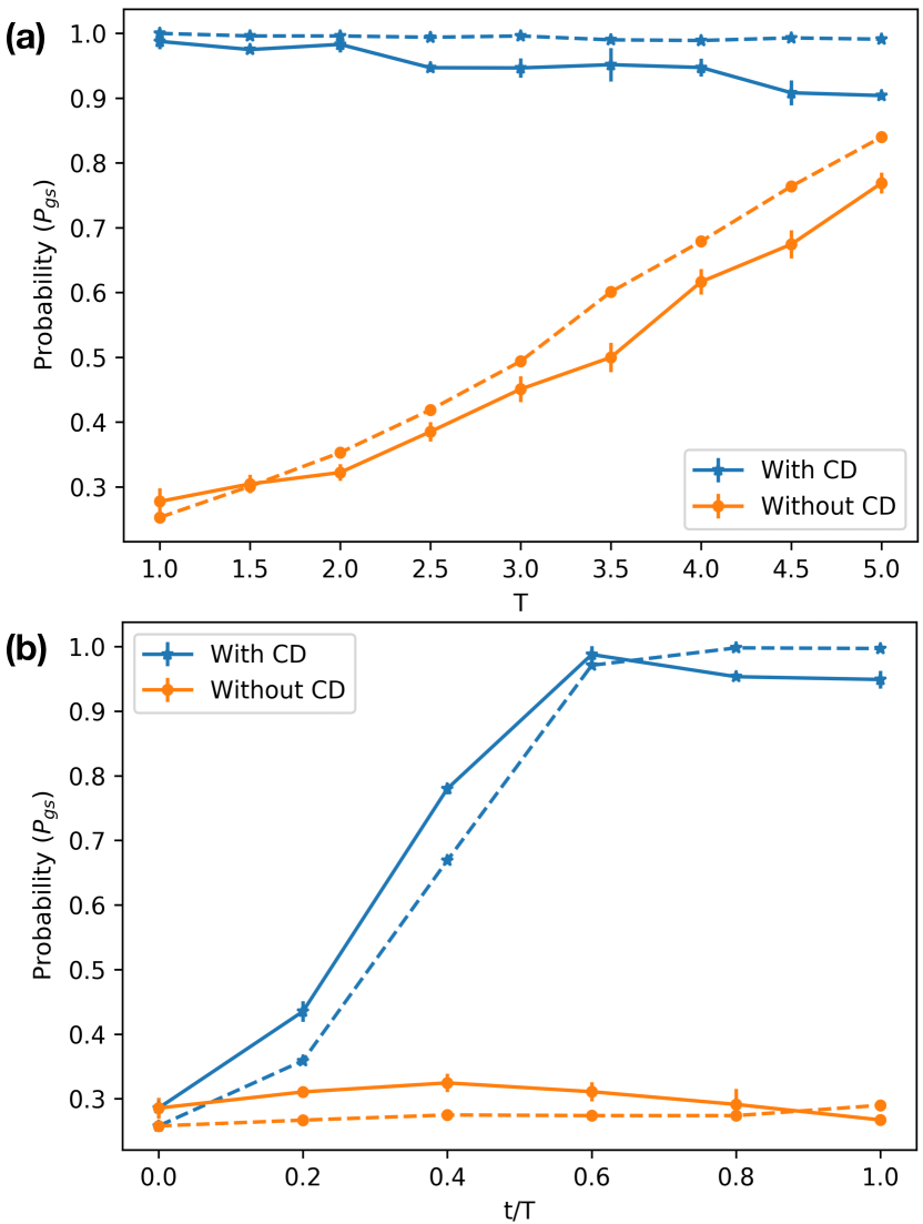
As an example, we consider interacting two qubit system, where the time evolution for can be easily implemented by two qubit entangling gates and single qubit rotation gates. The general circuit for implementing the evolution using CD driving is shown in Fig. 1. The initial and the target states chosen for the evolution are and , respectively, which is inferred directly from the following parameters: , and . The time evolution for STA assisted DAdQC and DAdQC for two qubits are shown in Fig. 3. Again, like the single qubit case, one can achieve a high fidelity for the target state preparation. The result obtained from the ideal digital simulator, in Fig. 3(a), shows that, when the additional term is considered, the target state can be achieved with almost unit fidelity. Furthermore, when a single evolution is considered, as depicted in Fig. 3(b), the target state can be achieved substantially faster than adiabatic evolution. However, when implemented in the real experiment, fidelity around is achieved with the application of the CD term, where the fidelity in the computational basis is calculated as . The application of the CD term is more suitable when the evolution time is small. In principle, the fidelity should remain the same even if we increase the number of time steps. Nevertheless, due to limited coherence time and the increasing number of gates required to implement the CD term, fidelity gradually decreases as depicted in Fig. 3(a).
III.0.2 Local CD from variational approach
A recently proposed method by Sels and Polkovnikov Sels and Polkovnikov (2017), based on the variational approach, also provides an alternative to calculate the approximate CD Hamiltonian with only local terms. The method for this calculation is to choose an appropriate adiabatic gauge potential Kolodrubetz et al. (2017) and minimizing the action , where the operator is defined by (see Appendix B). The CD driving using this method is expressed as . Since the Hamiltonian contains only real values in the -basis, the simplest ansatz is to choose , i.e., applying an additional magnetic field along the y-direction for each spin. By minimizing the action with respect to , the variational coefficient is analytically calculated, which takes the general form, for Eq. (6) Sels and Polkovnikov (2017),
| (9) |
The expression for is similar to that of Eq. (7) except for a few modifications. In Fig. 4(a), the probabilities of obtaining the ground state, from both the ideal simulator and the experimentally implemented data from ibmqx2 are shown for up to 5 qubits. Like the previous case, the final ground state can be prepared using the additional with high fidelity. The ideal simulator data shows that the final probability, reaches almost unity for in five trotter steps, especially when is small. However, the implemented value differs from the simulator due to the device errors.
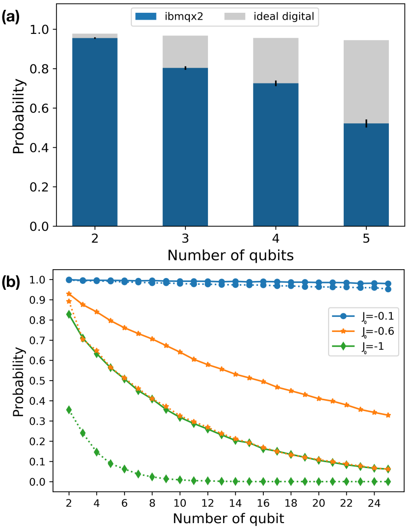
It should be noted that, in the above discussion, the interaction strength is kept sufficiently small compared to the external magnetic field, . The ground state of the final Hamiltonian is a ferromagnetic state, i.e., either or , depending on the sign of . In such scenario, the evolution assisted by the local CD terms in Eq. (7) and Eq. (9) produces the exact final ground state. Fig. 4(b) compares the probability of interacting multi-qubit system with ground state . For , the probability is around in the ideal simulator for both the methods. When becomes higher, the probability using Eq. (4) decreases drastically and reduces to , even for two qubits. Whereas, for the variational approach, the probability is significantly higher for large values. When the ground state is degenerate, the obtained result seems to differ from the actual ground state. For instance, when , with the similar values of other parameters, the ground state becomes doubly degenerate,i.e., the states and , the application of the CD term drives the system to one of the eigenstates. This comes out to be true for many spin systems also. Moreover, the calculation of the local CD term is based on the approximation that every spin is treated individually by considering an effective magnetic field acting upon each spin. The effects of the interaction are undermined while calculating the CD term. As a result, the CD term does not help the system evolve into the exact ground state when is comparable or stronger than that of the local magnetic field.
Subsequently, when , the final ground state becomes entangled, and one can deduce from Eq. (7) that for small , the CD term becomes small , i.e, . In such cases, the final evolved state, in a short , does not match the adiabatic one. For the variational approach, the CD term vanishes altogether and can not be applied using such form. Therefore, if we are to prepare a highly entangled state, the single qubit approximation for the CD term is not a good choice. This drawback occurs as CD driving is calculated using the terms, which refers to driving a single qubit with the external magnetic field only. In fact, the spin-spin interaction term decides the final state here and the driving for coupling has to be incorporated. This enforces the fact that the direct approach from the first principle to find the local CD driving is not realistic and should contain other interactions such as and etc. Vinci and Lidar (2017).
IV Approximate counter-diabatic driving
Following the discussion in the preceding section, when complex many-body systems are considered, the calculation of the exact CD term becomes difficult. Also, the form of the CD term can be severely complicated with different non-local and many-body interaction terms. Besides, it becomes rather difficult to implement systems with such interactions on current quantum computers. Although, the local terms, see Eq. (9), from variational approach gives an optimal solution, it is not that useful for preparing entangled states, especially when . The nature of the CD term from variational calculation depends on the choice of appropriate adiabatic gauge potential . A recently proposed method gives a more general way to choose the gauge potential by using the nested commutator (NC) Claeys et al. (2019),
| (10) |
where determines the order of the expansion. Depending on the required accuracy, we can keep the number of variational coefficients small. If we consider only the first-order term, our ansatz will be , and the effective Hamiltonian can be written as,
| (11) |
where is the relevant CD term.
First of all, we apply this technique to non-integrable Ising spin model, described by the Hamiltonian in Eq. (6). Considering the two-qubit system (), we approximate CD term using first-order nested commutator,
| (12) |
with,
| (13) |
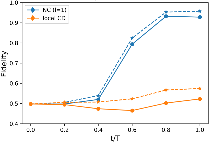
The second-order term () can give the exact gauge potential Claeys et al. (2019). However, for the experimental demonstration, we only consider the first-order term and implement the time evolution on a quantum processor. The circuit implementation for the CD driving is shown in Appendix A. Using this method, the final ground state is achieved with very few trotter steps compared to digitized adiabatic evolution, which drastically reduces the number of gates required as well as the total simulation time. In Fig. 5, we depicted the fidelity as a function of evolution time using first-order nested commutator method when the final ground state is degenerate and compared the result with the local CD term from Eq. (9). The fidelity is much better compared to the local CD case for degenerate state and thereby it justifies our argument in the preceding section.
Secondly, we shall check the reliability and validity as well as the extent of the variational approach in the many body regime. To this aim, we apply this technique to prepare the GHZ state in Ising spin chain with many spins, described by the Hamiltonian,
| (14) |
with being the number of spins. Here, the periodic boundary condition is assumed. Following the procedure described in Sec. IV, by considering only the first-order expansion, we calculate the approximate gauge potential as,
| (15) |
The variational coefficient, is calculated by minimizing the action . For the experimental demonstration on a quantum processor, we choose a small system with two and three qubits to prepare a Bell state and GHZ state. For the bell state, , governed by the Hamiltonian in Eq. (14), the variational coefficient is calculated as . Here we have noticed that, for two spins, the first order commutator is proportional to the higher-order terms. The resulting CD driving from the approximate gauge is exact and produces unit fidelity in ideal situations Claeys et al. (2019). The same procedure can be followed in case of more qubits to prepare a GHZ state starting from the qubit ground state . Specifically, the variational coefficient for a three-qubit case is given by .
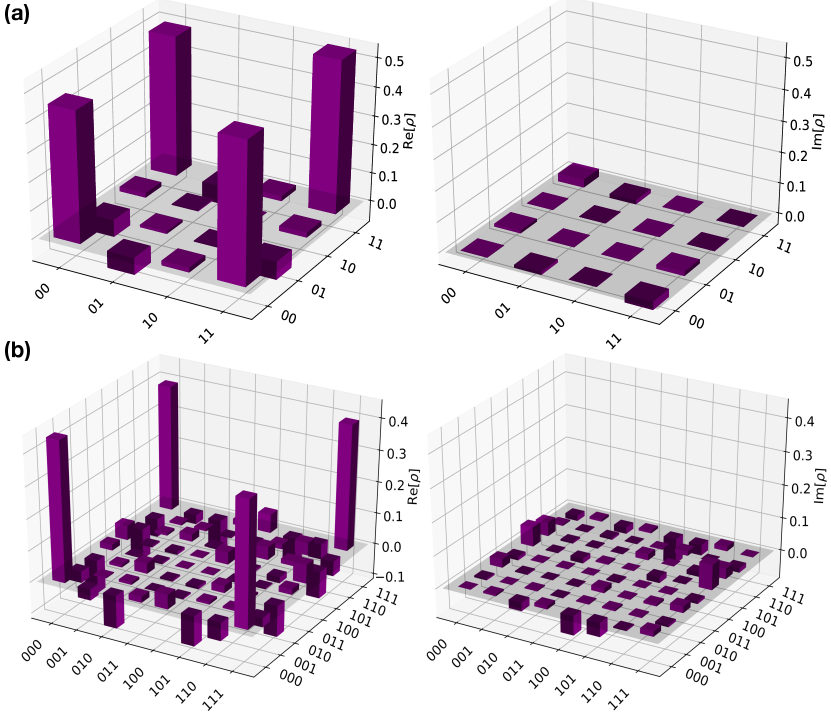
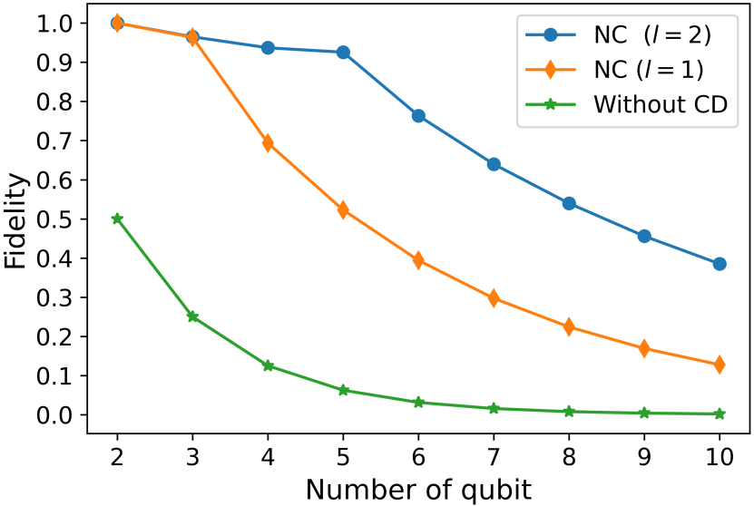
The simulation was performed on a five qubit quantum processor ibmq_ourense. A similar trotterization, as in Eq. (20), is used to study the evolution with digitized time step . Using the CD driving, with only three trotter steps, the desired bell state is obtained with experimental fidelity . The ideal digital simulation gives almost unit fidelity (). The fidelity is calculated as, , where the exact bell state is represented by, . Similarly, for the three-qubit system, the ideal digital evolution gives the fidelity with the exact GHZ state, and the corresponding experimental fidelity is . The density matrix representation of the final state () is obtained by performing quantum state tomography for both Bell and GHZ states and is depicted in Fig. 6. Whereas, Fig. 7, shows how the fidelity varies with increasing system size on a ideal digital simulator with six trotter steps. The first-order approximation of the CD term provides high fidelity for small system size. As we increase , the probability of obtaining the final ground state decreases gradually. This can be overcome by considering the higher-order commutators while calculating the approximate CD term. As the variational method tends to provide exact CD driving for larger -values, which in principle, can give a better fidelity in many-body systems.
V Conclusion
In conclusion, we have demonstrated the implementation of digitalized STA on a superconducting quantum processor. The problem Hamiltonian, chosen for the simulation, emulates the one-dimensional Ising spin chain. The STA is realized by means of the local and approximate CD driving, which is obtained using mainly two methods: the long-established Berry’s algorithm and the newly proposed variational approach. The CD term in our simulation is non-stoquastic in nature, therefore it can’t be simulated efficiently on a classical computer. The effective Hamiltonian is implemented using the available quantum gates, and the time evolution of the system is studied to achieve the ground state of the problem Hamiltonian. We have showed that the time steps required to reach the target state are minimal compared to the DAdQC method, leading to minimal loss due to the decoherences and accumulated gate errors. The local CD driving proved to be very effective for weakly interacting spin chains; however, is not useful in case of strong interaction and fails to produce degenerate target states. To remedy this situation, the approximate CD driving is useful, which can be calculated using the nested commutator method. We applied the first-order approximate CD term to prepare Bell and GHZ state with high fidelity for few qubit systems. Furthermore, for the many qubit systems, the fidelity can be further improved with higher-order terms at the cost of gate numbers.
This work provides the evidence that significant enhancement of the DAdQC approach can be achieved using the STA methods by decreasing the total computational cost and hence achieving the desired results within the coherence time of the device. To our knowledge, this work is the first to successfully realize the STA methods in a contemporary superconducting circuit-based quantum computer. Due to the decoherence and gate errors, the time evolution studies are challenging to perform in such devices. Our result provides a beginning to such studies on the speed up of AdQC algorithms.
Acknowledgement
The authors are grateful to Kazutaka Takahashi for useful discussions. We acknowledge support from National Natural Science Foundation of China (NSFC) (11474193), STCSM (2019SHZDZX01-ZX04, 18010500400 and 18ZR1415500), Program for Eastern Scholar, Ramón y Cajal program of the Spanish MCIU (RYC-2017-22482), QMiCS (820505) and OpenSuperQ (820363) of the EU Flagship on Quantum Technologies, Spanish Government PGC2018-095113-B-I00 (MCIU/AEI/FEDER, UE), Basque Government IT986-16, as well as the and EU FET Open Grant Quromorphic. This work is also partially supported from Huawei HiQ funding for developing QAOA&STA (Grant No. YBN2019115204).
Appendix A Method of digitization
The circuit model can efficiently simulate the adiabatic quantum computing by using the digitization of continuous adiabatic evolution. The time-dependent Hamiltonians, considered in this work, can be represented as a sum of -local terms that act on at most -qubits. This can be represented as
| (16) |
The continuous time evolution operator of is given by,
| (17) |
where is the time ordering operator. The discretization is done using the first order trotter-suzuki formula,
| (18) |
Here the total evolution time is divided into equal steps of width i.e., . In this case, the error would be of the order Suzuki (1976). One can also consider higher-order decomposition, which can give better approximation by minimizing the error further Hatano and Suzuki (2005). However, an interesting observation from our simulation is that the digital adiabatic evolution using CD driving is independent of the simulation time , and depends only on the number of trotter steps. So, by fixing the total time steps, we can choose an arbitrarily small value for and so that we can achieve arbitrary precision even with the first order trotterization. We ignore the time variation of the Hamiltonian on time scale lower than , which contributes to an extra error per each step. When the Hamiltonian fluctuation is very fast, it is possible to suppress this additional error, which is discussed in Poulin et al. (2011). From Eq. (18), the digital unitary evolution can be designed for the different Hamiltonians chosen in this work. For instance, one single step of TS decomposition for Eq. (5) will look like,
| (19) |
where , and , are the variables that represent the change in the Hamiltonian in each step. Similarly, for Eq. (8), four variables are required for each spin in each step, i.e.,
| (20) |
These unitary operators are implemented in the circuit model. According to the Solovay-Kitaev theorem Dawson and Nielsen (2005), any k-body unitary operation can be decomposed into a combination of single-qubit and two-qubit gate operations. Following are some example of the implementations, corresponding to the unitary operators used in this study,
![[Uncaptioned image]](https://cdn.awesomepapers.org/papers/209726a4-254c-4232-a0df-c1a15fc7955c/x8.png)
Appendix B Approximate CD term using variational method
The main idea of counter-diabatic driving is to add an auxiliary term to the original Hamiltonian and evolve the system according to an effective Hamiltonian,
| (21) |
where is the original Hamiltonian, is the control parameter, and is the exact adiabatic gauge potential responsible for the diabatic transitions. For the spin model considered in our simulation, the calculation of exact gauge potential results in non-local m-body interaction terms. Even though it is possible to implement these interactions using a basic set of quantum gates, the required gates will be huge and increase rapidly with the system size. Instead, for the practical purpose, we consider approximate gauge potential , which satisfies the equation,
| (22) |
For the optimal solution, we have to minimize the operator distance between the exact gauge potential and the approximate gauge potential, which is equivalent to minimizing the action,
| (23) |
where the Hilbert-Schmidt norm is given by,
| (24) |
A simple ansatz for for the Hamiltonian in Eq. (6) from the main-text is, . This single qubit approximation works very well even for many-body systems. However, when the spin interaction terms become the leading term of the adiabatic gauge potential, this ansatz fails. So, we consider a general way to choose the ansatz using sequence of nested commutators proposed in Claeys et al. (2019), that is,
| (25) |
from which, when , we will get the exact gauge potential.
| Circuit optimization | Fidelity | Gate Count | Expected gate error | ||
|---|---|---|---|---|---|
| Ideal | Experiment | Rotation | CNOT | ||
| Bell state preparation | |||||
| Optimized | 0.999 | 0.9835 | 8 | 2 | 0.01927 |
| Not optimized | 0.8021 | 19 | 14 | 0.11834 | |
| GHZ state preparation (3 qubit) | |||||
| Optimized | 0.9325 | 0.8198 | 20 | 7 | 0.07063 |
| Not optimized | 0.7370 | 23 | 15 | 0.14276 | |
Appendix C Error Analysis
Various errors significantly impact the outcomes of the experiments. The sources of errors can be divided into three main categories. (i) Discretization error arises due to the choice of in the trotterization process, (ii) Cumulative gate error is a combination of single qubit gate errors and CNOT errors and increases linearly with the circuit depth and (iii) Measurement error arises due to the measurements at the end of the time evolution. Also if the system evolves for a long time, as in the adiabatic case, the energy relaxation and dephasing also has to be considered. The cross-talks between the qubits and other environmental effects can also disturb our simulation, but these effects have not been considered in our simulations.
Discretization error:
In digital quantum simulation the main source of error arises from the discretization of the continuous time evolution of a Hamiltonian and decomposing this evolution into a sequence of quantum gates. The discretization can be performed using various methods, but the Trotter-Suzuki (TS) formula is the most widely used method among all because of its simplicity. In our simulation, we consider first order TS formula, where the error is of the order . For a given total time , we can choose an arbitrarily small value for to decrease the trotter error. However, with small , we need more trotter steps to reach the final time, which will increase the total gate count and eventually leads to accumulation of gate error. One possible solution for this problem is to consider a higher-order TS formula using extra gates Hatano and Suzuki (2005). Since the gate error is comparatively larger than the trotter error, we restrict ourselves to a first-order approximation.
| System | Trotter step | Rotation gates | CNOT gates | Fidelity | ||
| With CD | ||||||
| Single spin system | 2 | 7 | - | 0.995 | ||
|
4 | 70 | 40 | 0.993 | ||
| Bell-state preparation | 3 | 27 | 14 | 0.999 | ||
| GHZ state (3 qubit) | 4 | 111 | 60 | 0.966 | ||
| Without CD | ||||||
| Single spin system | 20 | 39 | - | 0.996 | ||
|
30 | 445 | 300 | 0.985 | ||
| Bell-state preparation | 24 | 70 | 48 | 0.998 | ||
| GHZ state (3 qubit) | 18 | 105 | 108 | 0.962 | ||
Gate error:
While implementing the time evolution of a system, gate error plays a crucial role. With increasing trotter steps, the gate error also increases linearly. The average fidelity of a single qubit and a CNOT gate of IBM quantum computer in our simulation is and , respectively. For the experimental implementation on a noisy device, it’s necessary to optimize the quantum circuit before sending it to the hardware to get the desired result. In our simulation, to decrease the gate error, we used transpilation function available in Qiskit Terra for circuit optimization. Table 1 shows the experimental fidelity for the preparation of Bell-state and GHZ state with circuit optimization and without circuit optimization. The gate count and the expected gate error is calculated in both cases. In Table 2, the gate counts for the successful implementation of the adiabatic evolution for different systems on a digital quantum computer is illustrated. From the data, it is conclusive that the inclusion of the CD term can improve fidelity and reduce the total gate count.
Measurement error mitigation:
One of the main source of error in our simulation is the readout error of the device. In the following, we briefly discuss how to mitigate measurement error on a small system using matrix inversion method. For that, we have to find out the response matrix for the given device. To measure , we consider a set of calibration circuits using only X-gate. Let be the probability distribution for each possible states obtained from the quantum processor after measuring at the end. be the probability distribution without readout noise. Then we can obtain which is approximately equal to the by applying the matrix inversion on the obtained result, i.e.
| (26) |
This method works only when the measurement error is much larger than the single qubit gate error used for initial state preparation. This is true for IBMQ devices, where the average single qubit gate error is of the order of and the measurement error is of the order . In this work we use the tool provided by qiskit ignis qis for performing the measurement error mitigation. More advanced methods can be found in Maciejewski et al. (2020).
References
- Feynman (1999) Richard P Feynman, “Simulating physics with computers,” Int. J. Theor. Phys 21 (1999).
- Georgescu et al. (2014) Iulia M Georgescu, Sahel Ashhab, and Franco Nori, “Quantum simulation,” Reviews of Modern Physics 86, 153 (2014).
- Houck et al. (2012) Andrew A Houck, Hakan E Türeci, and Jens Koch, “On-chip quantum simulation with superconducting circuits,” Nature Physics 8, 292 (2012).
- Lanyon et al. (2011) Ben P Lanyon, Cornelius Hempel, Daniel Nigg, Markus Müller, Rene Gerritsma, F Zähringer, Philipp Schindler, Julio T Barreiro, Markus Rambach, Gerhard Kirchmair, et al., “Universal digital quantum simulation with trapped ions,” Science 334, 57–61 (2011).
- Gerritsma et al. (2010) Rene Gerritsma, Gerhard Kirchmair, Florian Zähringer, E Solano, R Blatt, and CF Roos, “Quantum simulation of the dirac equation,” Nature 463, 68–71 (2010).
- Biamonte et al. (2017) Jacob Biamonte, Peter Wittek, Nicola Pancotti, Patrick Rebentrost, Nathan Wiebe, and Seth Lloyd, “Quantum machine learning,” Nature 549, 195–202 (2017).
- Lloyd et al. (2013) Seth Lloyd, Masoud Mohseni, and Patrick Rebentrost, “Quantum algorithms for supervised and unsupervised machine learning,” arXiv preprint arXiv:1307.0411 (2013).
- Dunjko et al. (2016) Vedran Dunjko, Jacob M Taylor, and Hans J Briegel, “Quantum-enhanced machine learning,” Physical review letters 117, 130501 (2016).
- Schuld and Killoran (2019) Maria Schuld and Nathan Killoran, “Quantum machine learning in feature hilbert spaces,” Physical review letters 122, 040504 (2019).
- Moll et al. (2018) Nikolaj Moll, Panagiotis Barkoutsos, Lev S Bishop, Jerry M Chow, Andrew Cross, Daniel J Egger, Stefan Filipp, Andreas Fuhrer, Jay M Gambetta, Marc Ganzhorn, et al., “Quantum optimization using variational algorithms on near-term quantum devices,” Quantum Science and Technology 3, 030503 (2018).
- Farhi and Harrow (2016) Edward Farhi and Aram W Harrow, “Quantum supremacy through the quantum approximate optimization algorithm,” arXiv preprint arXiv:1602.07674 (2016).
- Arute et al. (2020) Frank Arute, Kunal Arya, Ryan Babbush, Dave Bacon, Joseph C Bardin, Rami Barends, Sergio Boixo, Michael Broughton, Bob B Buckley, David A Buell, et al., “Quantum approximate optimization of non-planar graph problems on a planar superconducting processor,” arXiv preprint arXiv:2004.04197 (2020).
- Gisin et al. (2002) Nicolas Gisin, Grégoire Ribordy, Wolfgang Tittel, and Hugo Zbinden, “Quantum cryptography,” Reviews of modern physics 74, 145 (2002).
- Bennett and Brassard (2014) Charles H. Bennett and Gilles Brassard, “Quantum cryptography: Public key distribution and coin tossing,” Theoretical Computer Science 560, 7–11 (2014).
- Arute et al. (2019) Frank Arute, Kunal Arya, Ryan Babbush, Dave Bacon, Joseph C Bardin, Rami Barends, Rupak Biswas, Sergio Boixo, Fernando GSL Brandao, David A Buell, et al., “Quantum supremacy using a programmable superconducting processor,” Nature 574, 505–510 (2019).
- Farhi et al. (2001) Edward Farhi, Jeffrey Goldstone, Sam Gutmann, Joshua Lapan, Andrew Lundgren, and Daniel Preda, “A quantum adiabatic evolution algorithm applied to random instances of an np-complete problem,” Science 292, 472–475 (2001).
- Ambainis and Regev (2004) Andris Ambainis and Oded Regev, “An elementary proof of the quantum adiabatic theorem,” arXiv preprint quant-ph/0411152 (2004).
- Young et al. (2010) AP Young, S Knysh, and VN Smelyanskiy, “First-order phase transition in the quantum adiabatic algorithm,” Physical review letters 104, 020502 (2010).
- Peng et al. (2008) Xinhua Peng, Zeyang Liao, Nanyang Xu, Gan Qin, Xianyi Zhou, Dieter Suter, and Jiangfeng Du, “Quantum adiabatic algorithm for factorization and its experimental implementation,” Physical review letters 101, 220405 (2008).
- Reichardt (2004) Ben W. Reichardt, “The quantum adiabatic optimization algorithm and local minima,” (Association for Computing Machinery, 2004) p. 502–510.
- Steffen et al. (2003) Matthias Steffen, Wim van Dam, Tad Hogg, Greg Breyta, and Isaac Chuang, “Experimental implementation of an adiabatic quantum optimization algorithm,” Physical Review Letters 90, 067903 (2003).
- Bapst et al. (2013) Victor Bapst, Laura Foini, Florent Krzakala, Guilhem Semerjian, and Francesco Zamponi, “The quantum adiabatic algorithm applied to random optimization problems: The quantum spin glass perspective,” Physics Reports 523, 127–205 (2013).
- Das and Chakrabarti (2008) Arnab Das and Bikas K Chakrabarti, “Colloquium: Quantum annealing and analog quantum computation,” Reviews of Modern Physics 80, 1061 (2008).
- Johnson et al. (2011) Mark W Johnson, Mohammad HS Amin, Suzanne Gildert, Trevor Lanting, Firas Hamze, Neil Dickson, Richard Harris, Andrew J Berkley, Jan Johansson, Paul Bunyk, et al., “Quantum annealing with manufactured spins,” Nature 473, 194–198 (2011).
- Boixo et al. (2013) Sergio Boixo, Tameem Albash, Federico M Spedalieri, Nicholas Chancellor, and Daniel A Lidar, “Experimental signature of programmable quantum annealing,” Nature communications 4, 1–8 (2013).
- Aharonov et al. (2008) Dorit Aharonov, Wim Van Dam, Julia Kempe, Zeph Landau, Seth Lloyd, and Oded Regev, “Adiabatic quantum computation is equivalent to standard quantum computation,” SIAM review 50, 755–787 (2008).
- Barends et al. (2016) Rami Barends, Alireza Shabani, Lucas Lamata, Julian Kelly, Antonio Mezzacapo, Urtzi Las Heras, Ryan Babbush, Austin G Fowler, Brooks Campbell, Yu Chen, et al., “Digitized adiabatic quantum computing with a superconducting circuit,” Nature 534, 222–226 (2016).
- Torrontegui et al. (2013) Erik Torrontegui, Sara Ibáñez, Sofia Martínez-Garaot, Michele Modugno, Adolfo [del Campo], David Guéry-Odelin, Andreas Ruschhaupt, Xi Chen, and Juan Gonzalo Muga, “Chapter 2 - shortcuts to adiabaticity,” (Academic Press, 2013) pp. 117 – 169.
- Guéry-Odelin et al. (2019) D. Guéry-Odelin, A. Ruschhaupt, A. Kiely, E. Torrontegui, S. Martínez-Garaot, and J. G. Muga, “Shortcuts to adiabaticity: Concepts, methods, and applications,” Rev. Mod. Phys. 91, 045001 (2019).
- Takahashi (2019) Kazutaka Takahashi, “Hamiltonian engineering for adiabatic quantum computation: Lessons from shortcuts to adiabaticity,” Journal of the Physical Society of Japan 88, 061002 (2019).
- Demirplak and Rice (2003) Mustafa Demirplak and Stuart A. Rice, “Adiabatic population transfer with control fields,” The Journal of Physical Chemistry A 107, 9937–9945 (2003).
- Demirplak and Rice (2005) Mustafa Demirplak and Stuart A. Rice, “Assisted adiabatic passage revisited,” The Journal of Physical Chemistry B 109, 6838–6844 (2005).
- Berry (2009) M V Berry, “Transitionless quantum driving,” Journal of Physics A: Mathematical and Theoretical 42, 365303 (2009).
- Chen et al. (2010) Xi Chen, A. Ruschhaupt, S. Schmidt, A. del Campo, D. Guéry-Odelin, and J. G. Muga, “Fast optimal frictionless atom cooling in harmonic traps: Shortcut to adiabaticity,” Phys. Rev. Lett. 104, 063002 (2010).
- Chen et al. (2011) Xi Chen, E. Torrontegui, and J. G. Muga, “Lewis-riesenfeld invariants and transitionless quantum driving,” Phys. Rev. A 83, 062116 (2011).
- Masuda and Nakamura (2008) Shumpei Masuda and Katsuhiro Nakamura, “Fast-forward problem in quantum mechanics,” Phys. Rev. A 78, 062108 (2008).
- Masuda and Nakamura (2010) Shumpei Masuda and Katsuhiro Nakamura, “Fast-forward of adiabatic dynamics in quantum mechanics,” Proceedings of the Royal Society of London A: Mathematical, Physical and Engineering Sciences 466, 1135–1154 (2010).
- Schaff et al. (2010) Jean-Fran çois Schaff, Xiao-Li Song, Patrizia Vignolo, and Guillaume Labeyrie, “Fast optimal transition between two equilibrium states,” Phys. Rev. A 82, 033430 (2010).
- An et al. (2016) Shuoming An, Dingshun Lv, Adolfo Del Campo, and Kihwan Kim, “Shortcuts to adiabaticity by counterdiabatic driving for trapped-ion displacement in phase space,” Nature communications 7, 12999 (2016).
- Du et al. (2016) Yan-Xiong Du, Zhen-Tao Liang, Yi-Chao Li, Xian-Xian Yue, Qing-Xian Lv, Wei Huang, Xi Chen, Hui Yan, and Shi-Liang Zhu, “Experimental realization of stimulated raman shortcut-to-adiabatic passage with cold atoms,” Nature communications 7, 1–7 (2016).
- Lucas (2014) Andrew Lucas, “Ising formulations of many np problems,” Frontiers in Physics 2, 5 (2014).
- del Campo et al. (2012) Adolfo del Campo, Marek M Rams, and Wojciech H Zurek, “Assisted finite-rate adiabatic passage across a quantum critical point: exact solution for the quantum ising model,” Physical review letters 109, 115703 (2012).
- Özgüler et al. (2018) A. Barı ş Özgüler, Robert Joynt, and Maxim G. Vavilov, “Steering random spin systems to speed up the quantum adiabatic algorithm,” Phys. Rev. A 98, 062311 (2018).
- Takahashi (2013) Kazutaka Takahashi, “Transitionless quantum driving for spin systems,” Physical Review E 87, 062117 (2013).
- Hartmann and Lechner (2019) Andreas Hartmann and Wolfgang Lechner, “Rapid counter-diabatic sweeps in lattice gauge adiabatic quantum computing,” New Journal of Physics 21, 043025 (2019).
- Petiziol et al. (2018) Francesco Petiziol, Benjamin Dive, Florian Mintert, and Sandro Wimberger, “Fast adiabatic evolution by oscillating initial hamiltonians,” Physical Review A 98, 043436 (2018).
- Opatrnỳ and Mølmer (2014) Tomáš Opatrnỳ and Klaus Mølmer, “Partial suppression of nonadiabatic transitions,” New Journal of Physics 16, 015025 (2014).
- Petiziol et al. (2019) Francesco Petiziol, Benjamin Dive, Stefano Carretta, Riccardo Mannella, Florian Mintert, and Sandro Wimberger, “Accelerating adiabatic protocols for entangling two qubits in circuit qed,” Physical Review A 99, 042315 (2019).
- Ji et al. (2019) Yunlan Ji, Ji Bian, Xi Chen, Jun Li, Xinfang Nie, Hui Zhou, and Xinhua Peng, “Experimental preparation of greenberger-horne-zeilinger states in an ising spin model by partially suppressing the nonadiabatic transitions,” Physical Review A 99, 032323 (2019).
- Zhou et al. (2020) Hui Zhou, Yunlan Ji, Xinfang Nie, Xiaodong Yang, Xi Chen, Ji Bian, and Xinhua Peng, “Experimental realization of shortcuts to adiabaticity in a nonintegrable spin chain by local counterdiabatic driving,” Physical Review Applied 13, 044059 (2020).
- Vinci and Lidar (2017) Walter Vinci and Daniel A Lidar, “Non-stoquastic hamiltonians in quantum annealing via geometric phases,” npj Quantum Information 3, 1–6 (2017).
- Takahashi (2017) Kazutaka Takahashi, “Shortcuts to adiabaticity for quantum annealing,” Physical Review A 95, 012309 (2017).
- Passarelli et al. (2020) G. Passarelli, V. Cataudella, R. Fazio, and P. Lucignano, “Counterdiabatic driving in the quantum annealing of the -spin model: A variational approach,” Phys. Rev. Research 2, 013283 (2020).
- Sieberer et al. (2019) Lukas M Sieberer, Tobias Olsacher, Andreas Elben, Markus Heyl, Philipp Hauke, Fritz Haake, and Peter Zoller, “Digital quantum simulation, trotter errors, and quantum chaos of the kicked top,” npj Quantum Information 5, 1–11 (2019).
- Suzuki (1976) Masuo Suzuki, “Generalized trotter’s formula and systematic approximants of exponential operators and inner derivations with applications to many-body problems,” Communications in Mathematical Physics 51, 183–190 (1976).
- (56) “Ibm quantum experience,” https://www.research.ibm.com/ibm-q/.
- Hatomura (2017) Takuya Hatomura, “Shortcuts to adiabaticity in the infinite-range ising model by mean-field counter-diabatic driving,” Journal of the Physical Society of Japan 86, 094002 (2017).
- Sels and Polkovnikov (2017) Dries Sels and Anatoli Polkovnikov, “Minimizing irreversible losses in quantum systems by local counterdiabatic driving,” Proceedings of the National Academy of Sciences 114, E3909–E3916 (2017).
- Kolodrubetz et al. (2017) Michael Kolodrubetz, Dries Sels, Pankaj Mehta, and Anatoli Polkovnikov, “Geometry and non-adiabatic response in quantum and classical systems,” Physics Reports 697, 1–87 (2017).
- Claeys et al. (2019) Pieter W. Claeys, Mohit Pandey, Dries Sels, and Anatoli Polkovnikov, “Floquet-engineering counterdiabatic protocols in quantum many-body systems,” Phys. Rev. Lett. 123, 090602 (2019).
- Hatano and Suzuki (2005) Naomichi Hatano and Masuo Suzuki, “Finding exponential product formulas of higher orders,” (Springer, 2005) pp. 37–68.
- Poulin et al. (2011) David Poulin, Angie Qarry, Rolando Somma, and Frank Verstraete, “Quantum simulation of time-dependent hamiltonians and the convenient illusion of hilbert space,” Physical review letters 106, 170501 (2011).
- Dawson and Nielsen (2005) Christopher M Dawson and Michael A Nielsen, “The solovay-kitaev algorithm,” arXiv preprint quant-ph/0505030 (2005).
- (64) “Qiskit: An open-source framework for quantum computing,” https://qiskit.org/.
- Maciejewski et al. (2020) Filip B Maciejewski, Zoltán Zimborás, and Michał Oszmaniec, “Mitigation of readout noise in near-term quantum devices by classical post-processing based on detector tomography,” Quantum 4, 257 (2020).