This paper was converted on www.awesomepapers.org from LaTeX by an anonymous user.
Want to know more? Visit the Converter page.

Shifted shock formation for the 3D compressible Euler equations with damping and variation of the vorticity

Chen Zhendong111Acknowledgement: This is part of the Ph. D thesis of the author written under the supervision of Professor Zhouping Xin at the Institute of Mathematical Sciences of The Chinese University of Hong Kong. Institute of Mathematical Science, The Chinese University of Hong Kong, Shatin, NT, Hong Kong.
Abstract

In this paper, we consider the shock formation problem for the 3-dimensional(3D) compressible Euler equations with damping inspired by the work [4]. It will be shown that for a class of large data the damping can not prevent the formation of point shock and the damping effect shifts the shock time and the wave amplitude while the shock location and the blow up direction remain same with the information of this point shock being computed explicitly. Moreover, the vorticity is concentrated in the non-blow up direction which varies exponentially due to the damping effect. Our proof is based on the estimates for the modulated self-similar variables and lower bounds for the Lagrangian trajectories.

1 Introduction

We consider the following 3D Euler system with damping

tρ+uxρ=ρdivxutu+uxu=1ρxpautk+uxk=0,\begin{split}\partial_{t}\rho+u\cdot\nabla_{x}\rho&=-\rho div_{x}u\\ \partial_{t}u+u\cdot\nabla_{x}u&=-\dfrac{1}{\rho}\nabla_{x}p-au\\ \partial_{t}k+u\cdot\nabla_{x}k&=0,\end{split} (1.1)

with the space-time variables (t,x)=(t,x1,x2,x3)×3(t,x)=(t,x_{1},x_{2},x_{3})\in\mathbb{R}\times\mathbb{R}^{3}, the velocity u:×33u:\mathbb{R}\times\mathbb{R}^{3}\rightarrow\mathbb{R}^{3}, the positive density ρ:3×+\rho:\mathbb{R}^{3}\times\mathbb{R}\rightarrow\mathbb{R}_{+}, the entropy k:×3k:\mathbb{R}\times\mathbb{R}^{3}\rightarrow\mathbb{R} and the pressure p=p(ρ,k):×3+p=p(\rho,k):\mathbb{R}\times\mathbb{R}^{3}\rightarrow\mathbb{R}_{+} is given by

p(ρ,k)=1γργek.p(\rho,k)=\dfrac{1}{\gamma}\rho^{\gamma}e^{k}.

with the adiabatic constant γ>1\gamma>1. These equations describe the motion of a perfect fluid which follow from the conservation of mass, momentum and energy respectively. The term au-au on the right hand side of momentum equation represents the damping effect to the fluid with the damping constant a0a\neq 0.
     Instead of using the density, it’s convenient to rewrite the equation by the sound speed, which is defined as

c=pρ=ραek2,c=\sqrt{\dfrac{\partial p}{\partial\rho}}=\rho^{\alpha}e^{\frac{k}{2}},

where α=γ12.\alpha=\dfrac{\gamma-1}{2}. For simplicity, we denote σ\sigma to be the re-scaled sound speed

σ=1αc=1αραek2.\sigma=\dfrac{1}{\alpha}c=\dfrac{1}{\alpha}\rho^{\alpha}e^{\frac{k}{2}}.

Then, (1.1) can be rewritten as

tσ+uxσ+ασdivxu=0,tu+uxu+ασdivxσ=α2γσ2xkau,tk+uxk=0.\begin{split}\partial_{t}\sigma+u\cdot\nabla_{x}\sigma+\alpha\sigma div_{x}u&=0,\\ \partial_{t}u+u\cdot\nabla_{x}u+\alpha\sigma div_{x}\sigma&=\dfrac{\alpha}{2\gamma}\sigma^{2}\nabla_{x}k-au,\\ \partial_{t}k+u\nabla_{x}k&=0.\end{split} (1.2)

Define the specific vorticity ζ\zeta as ζ=ωρ=curluρ\zeta=\dfrac{\omega}{\rho}=\dfrac{curl\ u}{\rho}. Then, ζ\zeta satisfies the following equation:

tζ+uxζ=ζxu+αγσρxσ×xk=1ρ3xρ×xpaζ.\partial_{t}\zeta+u\cdot\nabla_{x}\zeta=\zeta\cdot\nabla_{x}u+\underbrace{\dfrac{\alpha}{\gamma}\dfrac{\sigma}{\rho}\nabla_{x}\sigma\times\nabla_{x}k}_{=\frac{1}{\rho^{3}}\nabla_{x}\rho\times\nabla_{x}p}-a\zeta. (1.3)

The first and second terms on the right-hand side of the equation(1.3) represent the consequences of vortex stretching and the baroclinic torque. The third term arises from the intersection of acoustic and entropy waves and results from the non-aligned pressure and density gradients. In the scenario where the system is isentropic, such that xρxp\nabla_{x}\rho\parallel\nabla_{x}p, this term vanishes. However, when the system is non-isentropic, this term plays a crucial role in the generation of vorticity. Irrotational data can produce vorticity instantaneously, as demonstrated in [4]. For example, if the density gradient is perpendicular to the pressure gradient, the lighter gas will be accelerated faster than the denser gas, resulting in the creation of vorticity.
     It is well-known that damping can prevent shock formation when the energy of the initial data is small. However, for large data sets, such as short pulse data or data with large energy, we will demonstrate that damping may not sufficiently prevent the formation of shock. Furthermore, we will show that the damping effect shift the time at which a shock occurs, while the blow-up location remains unchanged compared with the undamped case, with the degree of shift reliant on the value of aa.

1.1 Review of prior results for the Euler system

For the system(1.1), there are many studies both in 1D1D and multi-dimensions. For the one-dimensional Euler equations with damping, the global existence of smooth solutions with small data was proved by Nishida[21] and Slemrod[27] showed that for small data (LL^{\infty} sense), the 1D1D Euler equations with damping admit a global smooth solution while for large data, the equations can develop a shock in finite time. Later, these results were generalized by many authors, see [11, 22, 18, 17, 16, 23] and the references therein.
     In multi-dimensional case, the global existence and L2L^{2} estimates for the solutions to the 3D3D isentropic Euler system with damping was obtained by Kawashima[13]. Later, Sideris-Thomases-Wang in[26] showed that the size of the smooth initial data plays a key role for the lifespan to the 3D3D isentropic Euler equations with damping aρua\rho u. If the initial data are small, then damping can prevent the development of singularities; while if the initial data are large, the damping is not strong enough to prevent the formation of singularities in finite time. However, the authors in[26] only obtained the finite lifespan of the solutions and did not show the shock formation (including the shock mechanism) in finite time. The long time behavior of the solutions was obtained and generalized by many authors, see [29, 12, 24, 28, 26] and the references therein.
     In [6], Christodoulou achieved a significant breakthrough in understanding the shock mechanism for hyperbolic systems in three dimensions. Specifically, he considered the classical, non-relativistic, compressible Euler’s equations in three spatial dimensions, taking the data to be irrotational and isentropic. By imposing certain conditions on the initial data (i.e., the short pulse assumption), he obtained a complete geometric description of the maximal classical development. Notably, he provided a detailed analysis of the behavior of the solution at the boundary of the domain of the maximal classical solution, including a comprehensive description of its geometry. This work represents a significant advancement in understanding of shock formation in hyperbolic systems in three dimensions.
     In [25], Yu-Miao applied Christodoulou’s framework to the quasilinear wave equation in three spatial dimensions. By constructing a family of short pulse initial data that was first introduced by Christodoulou in [5], they demonstrated how the solution breaks down near the singularity and gave a sufficient condition on the initial data which leads to the shock formation in finite time. Additionally, J.Speck and J.Luk applied Christodoulou’s framework to the 2D Euler system without the assumption of irrotation. In [14], they studied plane-symmetric initial data with short pulse perturbation. For such initial data, they showed the shock mechanism such that the first derivatives of uu and ρ\rho blow up while uu and ρ\rho remain bounded near the shock. Then, in [15], they generalized these results to the 3D case. Specifically, they considered the 1D Euler equation of a simple small-amplitude solution as a plane-symmetric solution in 3D. They perturbed this solution in the (x2,x3)(x_{2},x_{3}) directions as a nearly plane-symmetric initial data for 3D isentropic Euler equations. They proved that the shock formation mechanism is stable under small and compactly supported perturbations with non-trivial vorticity and provided a precise description of the first singularity.
     Recently, Buckmaster, Shkoller, and Vicol published several results regarding shock formation in the multi-dimensional Euler system. Specifically, in their paper [3], they studied the 2D isentropic Euler equations under azimuthal symmetry (which differs from the 1D problem) with smooth initial data of finite energy and nontrivial vorticity. By utilizing modulated self-similar variables, they were able to obtain point shock forms in finite time, with explicit computation of the blow-up time and location. Furthermore, the solutions near the shock exhibit a cusp type.
     In a subsequent paper, [2], Buckmaster, Shkoller, and Vicol generalized their results to the 3D isentropic case for the ideal gas without any symmetry assumptions. In addition to the findings reported in [3], they were able to demonstrate the precise direction of blow-up and the geometric structure of the tangent surface of the shock profile. They also provided homogeneous Sobolev bounds for the fluid variables with an initial datum of large energy. Later, in[4], the authors extended their results to the full Euler equations. In this work, they primarily investigated the evolution and creation of vorticity, demonstrating that the vorticity remains bounded up to the shock formation. Notably, one of the primary differences between the isentropic and non-isentropic cases is the baroclinic torque in the equation of vorticity, which arises from the interaction between sound waves and entropy waves. Additionally, they constructed a set of irrotational data that results in the instantaneous creation of vorticity, which remains non-zero up to the shock.
     It is important to note that the point shock in the three aforementioned results is stable. That is, for any small, smooth, and generic perturbation of the given initial data, the corresponding Euler system results in a smooth solution that blows up in a small neighborhood of the original shock time and location. However, in [1], the authors demonstrated the existence of an open set of initial data that leads to the formation of an unstable shock. The primary difference between stable and unstable shocks is the set of background solutions for the self-similar variable WW, specifically the solutions of the various self-similar Burgers equations (3.43). For further details, one may refer to [9].
     The major tool used in the works mentioned above is the method of self-similar coordinates. This method was first introduced by Y.Giga and R.Kohn in [10] to study the asymptotic behavior of the solution to the nonlinear heat equation near the point of singularity. Y.Giga and R.Kohn considered the following nonlinear heat equation

utΔu|u|p1u=0,u_{t}-\Delta u-|u|^{p-1}u=0, (1.4)

where p>1p>1 and (x,t)n×(1,0)(x,t)\in\mathbb{R}^{n}\times(-1,0). They aimed to show the behavior of the solution near the singularity. To this end, they proposed the following self-similar transformation222Note that the transformation degenerates at t=0t=0.:

y=e12sx,s=ln(t),w(y,s)=e12(p1)su(x,t),y=e^{\frac{1}{2}s}x,\hskip 14.22636pts=-\ln(-t),\hskip 14.22636ptw(y,s)=e^{-\frac{1}{2(p-1)}s}u(x,t), (1.5)

which transforms (1.4) into

wsΔw+12yyw+1p1w|w|p1w=0.w_{s}-\Delta w+\frac{1}{2}y\cdot\nabla_{y}w+\frac{1}{p-1}w-|w|^{p-1}w=0. (1.6)

This transformation is motivated by the scaling property of (1.4). That is, for any uu solves (1.4), uλ:=λ2p1u(λx,λ2t)u_{\lambda}:=\lambda^{\frac{2}{p-1}}u(\lambda x,\lambda^{2}t) solves (1.4) as well. Based on the analysis of (1.6), they were able to demonstrate the asymptotic behavior of uu near the blow-up point (0,0)(0,0). Later, such method has been applied to various other dynamical systems, including the Scho¨\ddot{o}dinger equation [19], the Prandtl equations [7], the transverse viscous Burgers equation [8], and the semilinear wave equation [20]. The method of self-similar variables can provide precise information about the singularity of a given system by adding modulation variables to enforce certain orthogonality conditions and track the position of the singularity. It can also be used to characterize the type of singularities present, such as stable fixed points or center manifold and etc…, based on the behavior of the solutions near the singularity. For example, the stable shock in [3], [2], and [4] is based on the fact that the solutions approach the background solution near the shock exponentially with respect to the self-similar variables. For further details, one may refer to [9].

1.2 Outline

In section 2, the fundamental ideas of [2] and [4] will be illustrated by applying them to the standard Burgers equation and the Burgers equation with damping. Our results will demonstrate that the modulated variables can accurately track the location and time of the shock, and that the damping effect only shifts the blow-up time while leaving the blow-up location unchanged compared with the undamped case.
     Section 3 is devoted to reformulating of the Euler system (1.1) into its modulated self-similar version (3.28) by adapting the framework of [4]. Additionally, we extend the solution of the self-similar Burgers equation, which is introduced in Section 2, to three dimensions and derive higher-order derivatives of the evolution equations for the self-similar variables (W,Z,A,K)(W,Z,A,K).
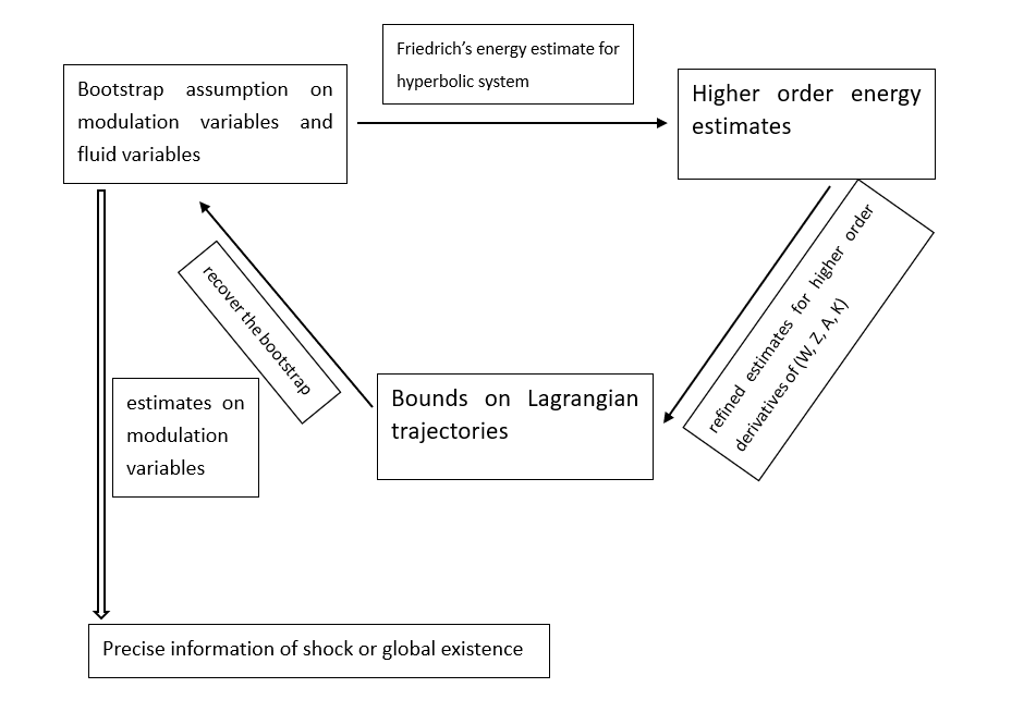
     In Section 4, we present an explicit construction of the initial datum in [4]. Note that the initial data for variable WW is dependent on the background solution W¯\bar{W}, which is a refined solution of the self-similar Burgers equation. Furthermore, we outline the self-similar Bootstrap assumptions for various variables and their derivatives, including the modulation variables and the self-similar variables (W,Z,A,K)(W,Z,A,K). These assumptions are more restrictive than the initial data constructed earlier and will be recovered in the subsequent sections. Finally, we state the main theorem (Theorem 4.1) of the paper at the end of this section.
     In Section 5, we present multiple estimates based on bootstrap assumptions, including the estimation of damping and forcing terms. Additionally, we state the H˙m\dot{H}^{m} energy bounds for (W,Z,A,K)(W,Z,A,K), whose proof solely relies on the bootstrap assumptions and the Friedrich’s energy estimates for the hyperbolic system. These estimates lead to higher-order derivatives estimates for (W,Z,A,K)(W,Z,A,K), which in turn help to further refine the estimates for the forcing terms.
     Section 6 is a key aspect of our work. In this section, we recover the bootstrap assumptions for the modulation variables under 10 constraints regarding γW(0,s)\partial^{\gamma}W(0,s), where |γ|2|\gamma|\leq 2. These constraints are initially satisfied and remain valid over time as long as the estimates for the modulation variables hold. In addition, it will be clearly shown that how the damping effect can influence the information of shock within this section.
     In Section 7, we derive lower bounds for the Lagrangian trajectories and introduced the crucial lemma7.2, which provides the key estimate required for recovering the remaining bootstrap assumptions. Moreover, we investigate the evolution of the vorticity, which is concentrated on the non-blow up direction, and demonstrated how it is affected by the damping effect. Inspired the work in[4], it will be shown that the initial region which genuinely affects the shock formation.
     By following the estimates presented in sections 5 to 7, we are able to recover the bootstrap assumptions for (W,Z,A,K)(W,Z,A,K) as outlined in section 8. This recovery is based on the significant lemma 7.2 and the utilization of the weighted framework (8.9). Note that to recover the bootstrap assumption for 1Aν\partial_{1}A_{\nu}, one has to establish the relation between 1Aν\partial_{1}A_{\nu} and the specific vorticity Ων\Omega_{\nu}.
     Section 9 serves to establish the H˙m\dot{H}^{m} energy bounds for the self-similar variables, thereby concluding the proof for the main theorem 4.1. Instead of studying the system for (W,Z,A,K)(W,Z,A,K), we utilize various Sobolev inequalities to derive the energy bounds for the equations of the velocity UU, the pressure PP, and the entropy HH (as seen in (3.42)). This approach proves to be more convenient to apply the Friedrich’s energy estimates.

1.3 Notations

Through the whole paper, the following notations will be used unless stated otherwise.

  • Latin indices {i,j,k,l,}\{i,j,k,l,\cdots\} take the values 1,2,3,1,2,3, and Greek indices {α,β,γ,}\{\alpha,\beta,\gamma,\cdots\} take the values 2,32,3. Repeated indices are meant to be summed.

  • For a three-component vector vv, denote the last two components of vv simply as vˇ\check{v}. For example, one can rewrite the gradient operator as =(1,ˇ).\nabla=(\partial_{1},\check{\nabla}).

  • The convention fhf\lesssim h means that there exists a universal positive constant CC such that fChf\leq Ch. The convention ABA\sim B means that there exists a universal positive constant such that A=O(B)A=O(B).

  • For any function A(y,s)A(y,s), denote A0A^{0} to be A0=A0(s)=A(y,s)|y=0A^{0}=A^{0}(s)=A(y,s)|_{y=0}.

2 Shock formation for the Burger’s equation in self-similar fancy

We consider the following Cauchy problem for 1D Burger’s equation

{tu+uxu=0,u(x,t=1)=f(x).\left\{\begin{split}&\partial_{t}u+u\partial_{x}u=0,\\ &u(x,t=-1)=f(x).\end{split}\right. (2.1)

For simplicity, we assume additionally that f(0)=0f(0)=0 and minxf(x)=xf(0)=1\min\partial_{x}f(x)=\partial_{x}f(0)=-1333Indeed, once can assume generally that xf(0)=c<0\partial_{x}f(0)=-c<0. Then the framework here also applies by slightly modified, i.e. T=1+1cT_{\ast}=-1+\frac{1}{c} and x=0x_{\ast}=0, and the corresponding self-similar transformation becomes s=ln(1+1ct),y=xe32s.s=-\ln(-1+\frac{1}{c}-t),\quad y=xe^{\frac{3}{2}s}. (2.2) . Then by standard characteristic method, the solution of (2.1) will form a shock at time T=0T_{\ast}=0 and the location x=0x_{\ast}=0 with xu(0,t)\partial_{x}u(0,t)\rightarrow-\infty as t0t\to 0. However, this method has some drawbacks in the following sense:

  • Is there any singularity before t=0t=0 and whether xu\partial_{x}u is the first quantity which blows up or not?

  • How does the shock profile look like, and how does the solution behave near the singularity?

The above questions can be solved by using self-similar coordinates which is defined as follows:

s=ln(t),y=xe32s,s=-\ln(-t),\quad y=xe^{\frac{3}{2}s}, (2.3)

and the corresponding unknown is given as

u(x,t)=es2U(y,s).u(x,t)=e^{-\frac{s}{2}}U(y,s). (2.4)

Then, (2.1) is transformed as

(s12)U+(32y+U)yU=0.(\partial_{s}-\dfrac{1}{2})U+(\dfrac{3}{2}y+U)\partial_{y}U=0. (2.5)
Remark 2.1.

In general, the self-similar transformation should be

s=ln(τ(t)t),y=(xξ(t))eαs,u(x,t)=eβsU(y,s),s=-\ln(\tau(t)-t),y=(x-\xi(t))e^{\alpha s},u(x,t)=e^{-\beta s}U(y,s), (2.6)

where the parameters τ(t)\tau(t) and ξ(t)\xi(t) represent the shock time and location, respectively. Here, one already knows the blow-up point is (0,0)(0,0), which means one could take τ(t)=ξ(t)=0\tau(t)=\xi(t)=0. Then, substituting (2.6) into (2.5) yields

(sβ)U+[αy+U]e(αβ1)syU=0.(\partial_{s}-\beta)U+[\alpha y+U]e^{(\alpha-\beta-1)s}\partial_{y}U=0. (2.7)

In order to guarantee the global existence of (2.7), one has to choose

α=β+1.\alpha=\beta+1. (2.8)

The choice of β=12\beta=\dfrac{1}{2} is used to guarantee the stability of shock.444This means the solution of (2.1) is approaching exponentially to the solution of the self-similar Burger’s equation (see(2.12)) in self-similar variable ss, i.e. limt0|u(x,t)(t)12U¯(x(t)32)|=0,x,\lim_{t\to 0}|u(x,t)-(-t)^{\frac{1}{2}}\bar{U}(\frac{x}{(-t)^{\frac{3}{2}}})|=0,\quad\forall\ x\in\mathbb{R}, (2.9) where U¯\bar{U} is given by (2.13). See[9] for more details.

Note that the Jacobian of the transformation is given by

(y,s)(x,t)=|e32s32yes0es|=e52s=1(t)52.\dfrac{\partial(y,s)}{\partial(x,t)}=\left|\begin{array}[]{cc}e^{\frac{3}{2}s}&\frac{3}{2}ye^{s}\\ 0&e^{s}\end{array}\right|=e^{\frac{5}{2}s}=\dfrac{1}{(-t)^{\frac{5}{2}}}. (2.10)

Hence, the self-similar transformation degenerates as t0t\to 0. Later we will prove that (2.7) admits a global solution on [0,)[0,\infty), and therefore, the only possibility of singularity formation is the transformation between the Cartesian coordinates and the self-similar coordinates becomes degenerated.
     Moreover, one can show that U(y,s)U(y,s) converges to U¯\bar{U} pointwisely as ss\to\infty. That is

lims|U(y,s)U¯(y)|=0,yR,\lim_{s\to\infty}|U(y,s)-\bar{U}(y)|=0,\quad\forall y\in R, (2.11)

where U¯\bar{U} is the solution of the following self-similar Burger’s equation

12U¯+(32y+U¯)yU¯=0.-\dfrac{1}{2}\bar{U}+\left(\dfrac{3}{2}y+\bar{U}\right)\partial_{y}\bar{U}=0. (2.12)

Indeed, U¯\bar{U} can be solved as a implicit function as

y=U¯U¯3,y(,),y=-\bar{U}-\bar{U}^{3},\hskip 14.22636pty\in(-\infty,\infty), (2.13)

which is globally defined.
     Hence, uxu_{x} blows up only at the shock point and location, i.e.

limt0xu(0,t)=limt0esyU(0,s)=limt01t,\lim_{t\to 0}\partial_{x}u(0,t)=\lim_{t\to 0}e^{s}\partial_{y}U(0,s)=\lim_{t\to 0}-\dfrac{1}{t}\to-\infty, (2.14)

and all the other quantities are bounded666Obviously, |u(x,t)|1|u(x,t)|\lesssim 1 and it can be shown that for any z0z\neq 0, limt0|xu(z,t)|1z23.\lim_{t\to 0}|\partial_{x}u(z,t)|\lesssim\frac{1}{z^{\frac{2}{3}}}.. The behavior of the solution near shock is given as

u(x,t)=(t)12U¯(x(t)32).u(x,t)=(-t)^{\frac{1}{2}}\bar{U}\left(\frac{x}{(-t)^{\frac{3}{2}}}\right). (2.15)
Remark 2.2.

To obtain the global existence of (2.5), one can check that if one defines the characteristics as

dYds=U(Y,s)+32Y,Y(0)=y0,\dfrac{dY}{ds}=U(Y,s)+\dfrac{3}{2}Y,\hskip 14.22636ptY(0)=y_{0},

along which UY=es2U0(y0)U\circ Y=e^{\frac{s}{2}}U_{0}(y_{0}), then e3s2Y=y0+(1es)U0(y0)e^{-\frac{3s}{2}}Y=y_{0}+(1-e^{-s})U_{0}(y_{0}), which means UU can be solved implicitly as U(y,s)=es2U0(e3s2yes2(1es)U)U(y,s)=e^{\frac{s}{2}}U_{0}\left(e^{-\frac{3s}{2}}y-e^{-\frac{s}{2}}(1-e^{-s})U\right). In order to require UU to be defined globally, it suffices to show

1+(1es)U00.1+(1-e^{-s})U^{\prime}_{0}\neq 0. (2.16)

This is guaranteed by assumption on the initial data.

2.1 The geometric structure of shock front

Consider the Surface Γ:(x,t,u(x,t))\Gamma:(x,t,u(x,t)) in R3R^{3}. Then, the normal vector NN of Γ\Gamma and the Gauss curvature KK of Γ\Gamma at each point are given as follows

N=J1(ux,ut,1),K=ux4(1+ut2+ux2)2,N=J^{-1}(-u_{x},-u_{t},1),\hskip 14.22636ptK=\dfrac{-u_{x}^{4}}{(1+u_{t}^{2}+u_{x}^{2})^{2}}, (2.17)

where J=1+ux2+ut2J=\sqrt{1+u_{x}^{2}+u_{t}^{2}}. Initially, N0=12(1,0,1)N_{0}=\dfrac{1}{\sqrt{2}}(1,0,1), K0=14K_{0}=-\dfrac{1}{4}. In the self-similar coordinate, consider the evolutions of N,KN,K at y=0y=0,

N\displaystyle N =11+e2sUy2+esU2Uy2(esUy,es2UUy,1)|,y=0\displaystyle=\dfrac{1}{\sqrt{1+e^{2s}U_{y}^{2}+e^{s}U^{2}U_{y}^{2}}}\left(-e^{s}U_{y},-e^{\frac{s}{2}}UU_{y},1\right)\left|{}_{y=0}\right., (2.18)
K\displaystyle K =1(1+e2sUy2+esU2)2|.y=0\displaystyle=-\dfrac{1}{(1+e^{-2s}U_{y}^{-2}+e^{-s}U^{2})^{2}}\left|{}_{y=0}\right.. (2.19)

Then, as ss\to\infty (t0t\to 0), since Uy(0,s)1U_{y}(0,s)\to-1, U(0,s)U¯(0)=0U(0,s)\to\bar{U}(0)=0, it holds that

N(1,0,0),K1.N\to(-1,0,0),\hskip 14.22636ptK\to-1. (2.20)

Therefore, shock formation to the Burgers’ equation (2.1) is equivalent to that

  • the transformation between the physical variables (the Cartesian coordinates) and the self-similar coordinates becomes degenerate;

  • the normal N(t)N(t) of the shock front become horizontal at shock point.

2.2 Shifted singularity for the Burgers’ equation with damping

We consider the following Cauchy problem for 1D Burgers’ equation with damping:

{tu+uxu=au,u(x,t=1)=f(x),\left\{\begin{split}&\partial_{t}u+u\partial_{x}u=-au,\\ &u(x,t=-1)=f(x),\end{split}\right. (2.21)

where a0a\neq 0 is the damping constant and f(x)f(x) is the same as in (2.1). It will be shown that when a<1a<1, the damping effect is small and (2.21) behaves like the standard Burgers’ equation such that smooth data can form a shock in finite time. Moreover, the damping will shift the blow-up time according to the sign of aa as follows.

  • If 0<a<1=min1xf0<a<1=-\min\frac{1}{\partial_{x}f}, the damping will delay the formation of shock and the closer aa is to 11, the larger the blow-up time is;

  • if a<0a<0, then the blow-up time will be in advanced.

Precisely, the blow-up time can be clarified as T=1aln(1a)1T_{\ast}=-\frac{1}{a}\ln(1-a)-1777If one assumes generally that xf(0)=c\partial_{x}f(0)=-c, then the first case becomes that 0<a<1c0<a<\frac{1}{c} while T=1aln(1ac)1T_{\ast}=-\frac{1}{a}\ln(1-\frac{a}{c})-1. and in both case, the blow-up location remains the same compared with the undamped case (i.e. x=0x_{\ast}=0). When a1a\geq 1, the damping effect is strong enough and (2.21) admits a global solution on [1,)[-1,\infty). To this end, define the following self-similar coordinates888The choice of modulation variables τ(t)\tau(t) and ξ(t)\xi(t) is mainly dependent on the invariance of (2.21) under space translation and time translation. That is, given any x0,t0x_{0},t_{0}\in\mathbb{R}, then for any solution uu to (2.21), u~:=u(xx0,tt0)\tilde{u}:=u(x-x_{0},t-t_{0}) solves (2.21) as well.:

s=ln(τ(t)t),y=e32s(xξ(t)),u(x,t)=es2U(y,s),\begin{split}s&=-\ln(\tau(t)-t),\\ y&=e^{\frac{3}{2}s}(x-\xi(t)),\\ u(x,t)&=e^{-\frac{s}{2}}U(y,s),\end{split} (2.22)

where τ(t)\tau(t) and ξ(t)\xi(t) represent the blow-up time and location respectively, with the initial condition τ(1)=ξ(1)=0\tau(-1)=\xi(-1)=0. Note that the Jacobian of the transformation is given by

(y,s)(x,t)=|e32s0(1τ˙)es|=(1τ˙(t))1(τ(t)t)52.\dfrac{\partial(y,s)}{\partial(x,t)}=\left|\begin{array}[]{cc}e^{\frac{3}{2}s}&\ast\\ 0&(1-\dot{\tau})e^{s}\end{array}\right|=(1-\dot{\tau}(t))\dfrac{1}{(\tau(t)-t)^{\frac{5}{2}}}. (2.23)

Hence, the transformation will degenerate at time T=τ(T)T_{\ast}=\tau(T_{\ast}) (it will be shown that 1τ˙(t)>01-\dot{\tau}(t)>0) and is a diffeomorphism for t<τ(t)t<\tau(t). Then, (2.21) will be transformed into

(s12)U+(32y+U1τ˙es2ξ˙(t)1τ˙)yU=aesU1τ˙,\left(\dfrac{\partial}{\partial s}-\dfrac{1}{2}\right)U+\left(\dfrac{3}{2}y+\dfrac{U}{1-\dot{\tau}}-e^{\frac{s}{2}}\dfrac{\dot{\xi}(t)}{1-\dot{\tau}}\right)\partial_{y}U=-\dfrac{ae^{-s}U}{1-\dot{\tau}}, (2.24)

with the initial condition

U(y,0)=f(x),U(0,0)=0,yU(0,0)=1.U(y,0)=f(x),U(0,0)=0,\partial_{y}U(0,0)=-1. (2.25)

To obtain a global solution for (2.24) is similar to the former case999In this case, define the characteristics as dYds=32Y+11τ˙U(Y,s),Y(0)=y0,\dfrac{dY}{ds}=\frac{3}{2}Y+\frac{1}{1-\dot{\tau}}U(Y,s),\quad Y(0)=y_{0}, (2.26) along which UY=es2ea(τes+1)U0(y0):=g(s)U0(y0)U\circ Y=e^{\frac{s}{2}}e^{-a(\tau-e^{-s}+1)}U_{0}(y_{0}):=g(s)U_{0}(y_{0}). Then, UU can be solved implicitly as U(y,s)=g(s)U0(e32sy0se32s1τ˙g(s)𝑑s1g(s)U(y,s))U(y,s)=g(s)U_{0}(e^{-\frac{3}{2}s}y-\int_{0}^{s}\frac{e^{\frac{3}{2}s^{\prime}}}{1-\dot{\tau}}g(s^{\prime})ds^{\prime}\frac{1}{g(s)}U(y,s)). To show the global existence of UU, it suffices to show 1+1a(1ea(t+1))U00,s[0,),1+\frac{1}{a}(1-e^{-a(t+1)})U_{0}^{\prime}\neq 0,\quad\forall s\in[0,\infty), (2.27) which is guaranteed by the initial data and the definition of TT_{\ast} (see(2.30)).. Here, we focus on the evolutions of τ(t)\tau(t) and ξ(t)\xi(t). Differentiating (2.24) w.r.t yy yields

(s12)yU+(32+11τ˙yU)yU+(32y+U1τ˙es2ξ(t)˙1τ˙)y2U=aesyU1τ˙.\left(\dfrac{\partial}{\partial s}-\dfrac{1}{2}\right)\partial_{y}U+\left(\dfrac{3}{2}+\dfrac{1}{1-\dot{\tau}}\partial_{y}U\right)\partial_{y}U+\left(\dfrac{3}{2}y+\dfrac{U}{1-\dot{\tau}}-e^{\frac{s}{2}}\dfrac{\dot{\xi(t)}}{1-\dot{\tau}}\right)\partial_{y}^{2}U=-\dfrac{ae^{-s}\partial_{y}U}{1-\dot{\tau}}. (2.28)

Now we postulate that U(0,s)=0U(0,s)=0 and yU(0,s)=1\partial_{y}U(0,s)=-1 for all s[0,)s\in[0,\infty). This can be achieved by choosing τ(t)\tau(t) and ξ(t)\xi(t) suitably since initially, it holds that U(0,0)=0U(0,0)=0 and yU(0,0)=1\partial_{y}U(0,0)=-1. Evaluating (2.24) and (2.28) at y=0y=0 yields

{ξ˙(t)=0,τ˙(t)=aes=a(τ(t)t),\left\{\begin{split}&\dot{\xi}(t)=0,\\ &\dot{\tau}(t)=ae^{-s}=a(\tau(t)-t),\end{split}\right. (2.29)

which implies

{ξ(t)=ξ(1)=0,τ(t)=t+ea(1+t)+1a(1ea(1+t)).\left\{\begin{split}&\xi(t)=\xi(-1)=0,\\ &\tau(t)=t+e^{a(1+t)}+\dfrac{1}{a}(1-e^{a(1+t)}).\end{split}\right. (2.30)

To conclude, it holds that

  • if a1a\geq 1, then τ(t)t\tau(t)\geq t for all t1t\geq-1, and one obtains a global classical solution to (2.21);

  • if a<1a<1101010If one assumes generally that xf(0)=c\partial_{x}f(0)=-c, then this case becomes ”if a<1ca<\frac{1}{c}, then a shock forms at T=1aln(1ac)1T_{\ast}=-\dfrac{1}{a}\ln(1-\frac{a}{c})-1.” Therefore, for fixed aa, small data(i.e.c1ac\leq\frac{1}{a}) leads to the global solution while large data leads to the shock formation in finite time., then the transformation between Cartesian coordinates and self-similar coordinates will degenerate at time T=τ(T)T_{\ast}=\tau(T_{\ast}) which can be computed as T=1aln(1a)1T_{\ast}=-\dfrac{1}{a}\ln(1-a)-1, and

    limtTxu(ξ(t),t)=limtTesyU(0,s)=limtT1τ(t)t,\lim_{t\to T_{\ast}}\partial_{x}u(\xi(t),t)=\lim_{t\to T_{\ast}}e^{s}\partial_{y}U(0,s)=\lim_{t\to T_{\ast}}\dfrac{-1}{\tau(t)-t}\to-\infty, (2.31)

    i.e. the solution will form a shock at (x,t)=(0,T)(x,t)=(0,T_{\ast}). In this case, one sees that the blow-up location doesn’t shift.

2.3 Global existence to the Burgers’ equation

One can also use the self-similar coordinates to show the global existence to (2.1) with the initial data being everywhere increasing. For simplicity, we assume that xu0=xu(x,t=1)\partial_{x}u_{0}=\partial_{x}u(x,t=1)(start from t=1t=1) attains its min at x=0x=0 with xu0(0)0\partial_{x}u_{0}(0)\geq 0. Then, the classical results show that (2.1) admits a global ”rarefaction wave” solution. To this end, define the following self-similar transformation:

s=ln(t),y=e3s2x,u(x,t)=es2U(y,s).\begin{split}s&=\ln(t),\\ y&=e^{-\frac{3s}{2}}x,\\ u(x,t)&=e^{\frac{s}{2}}U(y,s).\end{split} (2.32)

Then, (2.1) is transformed into

(s+12)U+(U32y)yU=0,\left(\partial_{s}+\dfrac{1}{2}\right)U+\left(U-\dfrac{3}{2}y\right)\partial_{y}U=0, (2.33)

with the initial condition

yU(y,0)=yU0(y)=xu00.\partial_{y}U(y,0)=\partial_{y}U_{0}(y)=\partial_{x}u_{0}\geq 0. (2.34)

Note that in this case, the Jacobian of the transform is given as

(y,s)(x,t)=|e3s232yes0es|=e5s2=1t52>0,\dfrac{\partial(y,s)}{\partial(x,t)}=\left|\begin{array}[]{cc}e^{-\frac{3s}{2}}&-\dfrac{3}{2}ye^{-s}\\ 0&e^{-s}\end{array}\right|=e^{-\frac{5s}{2}}=\dfrac{1}{t^{\frac{5}{2}}}>0, (2.35)

which implies the transform (2.32) is a global diffeomorphism. Hence, if one obtains a global solution in the self-similar coordinates, then the global existence of original Burgers’ equation in Cartesian coordinates is automatically obtained. It can be shown in the similar way that (2.33) admits a global solution on s[0,)s\in[0,\infty) which converges to U^\hat{U} pointwisely,

lims|U(y,s)U^(y)|=0,y,\lim_{s\to\infty}|U(y,s)-\hat{U}(y)|=0,\quad\forall y\in\mathbb{R},

where U^=U^(y)\hat{U}=\hat{U}(y) is the solution of

12U^+(U^32y)yU^=0.\dfrac{1}{2}\hat{U}+(\hat{U}-\dfrac{3}{2}y)\partial_{y}\hat{U}=0. (2.36)

Indeed, U^\hat{U} can be solved implicitly as

y=U^+U^3,y(,+).y=\hat{U}+\hat{U}^{3},\hskip 14.22636pty\in(-\infty,+\infty). (2.37)

Then, for all x0x_{0}\in\mathbb{R}, it holds that

|xu(x0,t)|=es|yU(y0,s)|C1t,t1.|\partial_{x}u(x_{0},t)|=e^{-s}|\partial_{y}U(y_{0},s)|\leq C\dfrac{1}{t},\quad\forall t\geq 1. (2.38)
Remark 2.3.

It seems that the condition yU0(0)=xu0(0)0\partial_{y}U_{0}(0)=\partial_{x}u_{0}(0)\geq 0 which is the global minimum doesn’t use for the global existence of (2.33). However, one can check that if one defines the characteristics of (2.33) as

dYds=U(Y,s)32Y,Y(0)=y0,\dfrac{dY}{ds}=U(Y,s)-\dfrac{3}{2}Y,\hskip 14.22636ptY(0)=y_{0},

along which UY=es2U0(y0)U\circ Y=e^{-\frac{s}{2}}U_{0}(y_{0}), then e3s2Y=y0+U0(y0)(es1)e^{\frac{3s}{2}}Y=y_{0}+U_{0}(y_{0})(e^{s}-1), which allows one to solve UU implicitly as U(y,s)=es2U0(e3s2yes2(es1)U)U(y,s)=e^{-\frac{s}{2}}U_{0}\left(e^{\frac{3s}{2}}y-e^{\frac{s}{2}}(e^{s}-1)U\right). Then, this formula indeed defines a global solution UU provided

1+(es1)U00,1+(e^{s}-1)U_{0}^{\prime}\neq 0, (2.39)

which is guaranteed by the assumption on the initial data.

3 Coordinates transformations and the self-similar Euler system

To study the structure of shock front and introduce the self-similar coordinates, we will construct 10 modulation variables to control the following entities111111The choice of these modulation variables are derived from the invariance of the equations(1.1) under time re-scaling and Galilean transformations which including the space transformation, the time translation, the union motion (the shear transformation) and the space rotation.:

{the speed shock formationκ(t),the blow up timeτ(t),the blow up locationξ(t)3,the blow up directionn(t)3( only 2 freedoms),the tangent surface of shock frontϕ(t)3.\left\{\begin{split}&\text{the speed shock formation}\leftarrow\kappa(t)\in\mathbb{R},\\ &\text{the blow up time}\leftarrow\tau(t)\in\mathbb{R},\\ &\text{the blow up location}\leftarrow\xi(t)\in\mathbb{R}^{3},\\ &\text{the blow up direction}\leftarrow n(t)\in\mathbb{R}^{3}(\text{ only 2 freedoms}),\\ &\text{the tangent surface of shock front}\leftarrow\phi(t)\in\mathbb{R}^{3}.\end{split}\right. (3.1)

Then, the following coordinates transformations will be used:

original physical variables rotation,translationtime-rescalingthe Galilean coordinatesshear-transformation\displaystyle\text{original physical variables }\xrightarrow[\text{rotation,translation}]{\text{time-rescaling}}\text{the Galilean coordinates}\xrightarrow{\text{shear-transformation}}
flatted coordinates w.r.t the shock fronttransformationself-similarself-similar coordinates\displaystyle\text{flatted coordinates w.r.t the shock front}\xrightarrow[\text{transformation}]{\text{self-similar}}\text{self-similar coordinates}

3.1 The coordinates under Galilean transform

First, do time-rescaling as

tt=1+α2t,\mathrm{t}\rightarrow t=\dfrac{1+\alpha}{2}\mathrm{t},

so that all the modulation variables are defined w.r.t the rescaled time (i.e. tt).
     Given an unit vector n(t)=(1n22(t)n32(t),n2(t),n3(t))=(n1,n˘(t))n(t)=(\sqrt{1-n_{2}^{2}(t)-n_{3}^{2}(t)},n_{2}(t),n_{3}(t))=(n_{1},\breve{n}(t)), one can generate a rotation matrix which transforms e1e_{1} to n1(t)n_{1}(t). Precisely, let

R(t)=(n1n2n3n21n221+n1n2n31+n1n3n2n31+n11n321+n1).R(t)=\left(\begin{array}[]{ccc}n_{1}&-n_{2}&-n_{3}\\ n_{2}&1-\frac{n_{2}^{2}}{1+n_{1}}&-\frac{n_{2}n_{3}}{1+n_{1}}\\ n_{3}&-\frac{n_{2}n_{3}}{1+n_{1}}&1-\frac{n_{3}^{2}}{1+n_{1}}\end{array}\right). (3.2)

Then, the rotation matrix R(t)R(t) rotates e1e_{1} to n(t)n(t). Define the new coordinates as

(x~,t)=(RT(xξ(t)),t)(\tilde{x},t)=(R^{T}(\mathit{x}-\xi(t)),t) (3.3)

and the corresponding fluid variables as

σ~(x~,t)=σ(x,t),u~(x~,t)=RT(t)u(x,t),k~(x~,t)=k(x,t).\tilde{\sigma}(\tilde{x},t)=\sigma(\mathit{x},t),\quad\tilde{u}(\tilde{x},t)=R^{T}(t)u(\mathit{x},t),\quad\tilde{k}(\tilde{x},t)=k(x,t). (3.4)

Note that

t\displaystyle\dfrac{\partial}{\partial t} =1+α2t+v~x~i,\displaystyle=\dfrac{1+\alpha}{2}\dfrac{\partial}{\partial\mathit{t}}+\tilde{v}\dfrac{\partial}{\partial\tilde{x}_{i}}, (3.5)
xi\displaystyle\dfrac{\partial}{\partial\mathit{x}_{i}} =Rikx~k,\displaystyle=R_{ik}\dfrac{\partial}{\partial\tilde{x}_{k}}, (3.6)

where

v~=Q˙x~RTξ˙,Q˙=R˙TR,Q˙ij=Q˙ji.\tilde{v}=\dot{Q}\tilde{x}-R^{T}\dot{\xi},\quad\dot{Q}=\dot{R}^{T}R,\quad\dot{Q}_{ij}=-\dot{Q}_{ji}. (3.7)

Hence, the Euler system (1.2) is transformed in (x~,t)(\tilde{x},t) as

1+α2tσ~+(u~+v~)x~σ~+ασdivx~u~=0,1+α2tu~Q˙u~+(u~+v~)x~u~+ασ~x~σ~=α2γσ~2x~k~au~,1+α2tk~+(u~+v~)x~k~=0,\begin{split}\dfrac{1+\alpha}{2}\partial_{t}\tilde{\sigma}+(\tilde{u}+\tilde{v})\cdot\nabla_{\tilde{x}}\tilde{\sigma}+\alpha\sigma div_{\tilde{x}}\tilde{u}&=0,\\ \dfrac{1+\alpha}{2}\partial_{t}\tilde{u}-\dot{Q}\tilde{u}+(\tilde{u}+\tilde{v})\cdot\nabla_{\tilde{x}}\tilde{u}+\alpha\tilde{\sigma}\nabla_{\tilde{x}}\tilde{\sigma}&=\dfrac{\alpha}{2\gamma}\tilde{\sigma}^{2}\nabla_{\tilde{x}}\tilde{k}-a\tilde{u},\\ \dfrac{1+\alpha}{2}\partial_{t}\tilde{k}+(\tilde{u}+\tilde{v})\cdot\nabla_{\tilde{x}}\tilde{k}&=0,\end{split} (3.8)

together with the vorticity equation

1+α2tζ~Q˙ζ~+(u~+v~)x~ζ~ζ~x~u~=αγσ~ρ~x~σ~×x~k~aζ~.\dfrac{1+\alpha}{2}\partial_{t}\tilde{\zeta}-\dot{Q}\tilde{\zeta}+(\tilde{u}+\tilde{v})\cdot\nabla_{\tilde{x}}\tilde{\zeta}-\tilde{\zeta}\cdot\nabla_{\tilde{x}}\tilde{u}=\dfrac{\alpha}{\gamma}\dfrac{\tilde{\sigma}}{\tilde{\rho}}\nabla_{\tilde{x}}\tilde{\sigma}\times\nabla_{\tilde{x}}\tilde{k}-a\tilde{\zeta}. (3.9)

3.2 The flatted coordinates with respect to shock front

In order to see the geometry of the shock, define the ”tangent” quadratic surface as

(f(x~2,x~3,t),x~2,x~3),(f(\tilde{x}_{2},\tilde{x}_{3},t),\tilde{x}_{2},\tilde{x}_{3}), (3.10)

where ff is a quadratic form given as

f(x~˘,t)=12ϕαβx~αx~β,f(\breve{\tilde{x}},t)=\dfrac{1}{2}\phi_{\alpha\beta}\tilde{x}_{\alpha}\tilde{x}_{\beta}, (3.11)

with ϕ\phi being a symmetric 22-tensor. Then, define the shear transformation as

(x1,x2,x3)=(x~1f(x~1,x~2,t),x~2,x~3),(x_{1},x_{2},x_{3})=(\tilde{x}_{1}-f(\tilde{x}_{1},\tilde{x}_{2},t),\tilde{x}_{2},\tilde{x}_{3}), (3.12)

which flattens the ”tangent” surface. Note that together with the coordinates transform, the ”basis” (n(t),e~2=R(t)e2,e~3=R(t)e3)(n(t),\tilde{e}_{2}=R(t)e_{2},\tilde{e}_{3}=R(t)e_{3}) transforms automatically into

N(t)=J1(1,f,2,f,3),\displaystyle N(t)=J^{-1}(1,-f_{,2},-f_{,3}), (3.13)
T2=R(N(t))e2=(f,2J,1(f,2)2J(J+1),f,2f,3J(J+1)),\displaystyle T^{2}=R(N(t))e_{2}=\left(\dfrac{f_{,2}}{J},1-\dfrac{(f_{,2})^{2}}{J(J+1)},\dfrac{-f_{,2}f_{,3}}{J(J+1)}\right), (3.14)
T3=R(N(t))e3=(f,3J,f,2f,3J(J+1),1(f,3)2J(J+1)),\displaystyle T^{3}=R(N(t))e_{3}=\left(\dfrac{f_{,3}}{J},\dfrac{-f_{,2}f_{,3}}{J(J+1)},1-\dfrac{(f_{,3})^{2}}{J(J+1)}\right), (3.15)

where J>0J>0 and J2=1+|f,2|2+|f,3|2J^{2}=1+|f_{,2}|^{2}+|f_{,3}|^{2} and R(N(t))R(N(t)) is the rotation matrix generated by N(t)N(t) (with the role of n(t)n(t) replaced by N(t)N(t)).

Remark 3.1.

Note that the 2nd2^{nd} fundamental form of the ”tangent” surface is given by II=J1ϕαβdx~αdx~β\text{II}=J^{-1}\phi_{\alpha\beta}d\tilde{x}^{\alpha}d\tilde{x}^{\beta}. So, the functions ϕ\phi indeed reveal the geometry structure of the shock front.

Denote the corresponding fluid variables as

ů(x,t)\displaystyle\mathring{u}(x,t) =u~(x~,t),σ̊(x,t)=σ~(x~,t),k̊(x,t)=k~(x~,t),\displaystyle=\tilde{u}(\tilde{x},t),\quad\mathring{\sigma}(x,t)=\tilde{\sigma}(\tilde{x},t),\quad\mathring{k}(x,t)=\tilde{k}(\tilde{x},t),
v̊(x,t)\displaystyle\mathring{v}(x,t) =v~(x~,t),ζ̊(x,t)=ζ~(x~,t).\displaystyle=\tilde{v}(\tilde{x},t),\quad\mathring{\zeta}(x,t)=\tilde{\zeta}(\tilde{x},t).

Note that

t\displaystyle\dfrac{\partial}{\partial t} =tf˙x1,x~1=x1,x~α=xαf,αx1.\displaystyle=\dfrac{\partial}{\partial t}-\dot{f}\dfrac{\partial}{\partial x_{1}},\quad\dfrac{\partial}{\partial\tilde{x}_{1}}=\dfrac{\partial}{\partial x_{1}},\quad\dfrac{\partial}{\partial\tilde{x}_{\alpha}}=\dfrac{\partial}{\partial x_{\alpha}}-f_{,\alpha}\dfrac{\partial}{\partial x_{1}}.

Then, by defining the following constants

β1=11+α,β2=1α1+α,β3=α1+α,β4=β31+2α,\beta_{1}=\dfrac{1}{1+\alpha},\beta_{2}=\dfrac{1-\alpha}{1+\alpha},\beta_{3}=\dfrac{\alpha}{1+\alpha},\beta_{4}=\dfrac{\beta_{3}}{1+2\alpha}, (3.16)

the Euler system (3.8) is transformed into

tσ̊+2β1[JN(ů+v̊)f˙2β1]1σ̊+2β3(ůμ+v̊μ)μσ̊+2β3σ̊[1ůJN+μůμ]=0,tů2β1ůQ˙+2β1[JN(ů+v̊)f˙2β1]1ů+2β3(ůμ+v̊μ)μů+2β3σ̊[JN1+δμμ]σ̊=β4σ̊2[JN1+δμμ]k̊2β1aů,tk̊+2β1[JN(ů+v̊)f˙2β1]1k̊+2β3(ůμ+v̊μ)μk̊=0,\begin{split}&\partial_{t}\mathring{\sigma}+2\beta_{1}\left[JN\cdot(\mathring{u}+\mathring{v})-\dfrac{\dot{f}}{2\beta_{1}}\right]\partial_{1}\mathring{\sigma}+2\beta_{3}(\mathring{u}_{\mu}+\mathring{v}_{\mu})\partial_{\mu}\mathring{\sigma}+2\beta_{3}\mathring{\sigma}[\partial_{1}\mathring{u}\cdot JN+\partial_{\mu}\mathring{u}_{\mu}]=0,\\ &\partial_{t}\mathring{u}-2\beta_{1}\mathring{u}\dot{Q}+2\beta_{1}\left[JN\cdot(\mathring{u}+\mathring{v})-\dfrac{\dot{f}}{2\beta_{1}}\right]\partial_{1}\mathring{u}+2\beta_{3}(\mathring{u}_{\mu}+\mathring{v}_{\mu})\partial_{\mu}\mathring{u}+2\beta_{3}\mathring{\sigma}[JN\partial_{1}+\delta^{\cdot\mu}\partial_{\mu}]\mathring{\sigma}\\ &=\beta_{4}\mathring{\sigma}^{2}[JN\partial_{1}+\delta^{\cdot\mu}\partial_{\mu}]\mathring{k}-2\beta_{1}a\mathring{u},\\ &\partial_{t}\mathring{k}+2\beta_{1}\left[JN\cdot(\mathring{u}+\mathring{v})-\dfrac{\dot{f}}{2\beta_{1}}\right]\partial_{1}\mathring{k}+2\beta_{3}(\mathring{u}_{\mu}+\mathring{v}_{\mu})\partial_{\mu}\mathring{k}=0,\end{split} (3.17)

together with the vorticity equation

tζ̊2β1ζ̊Q˙+2β1[JN(ů+v̊)f˙2β1]1ζ̊+2β3(ůμ+v̊μ)μζ̊2β1[JNζ̊1ů+ζ̊μμů]=2β4σ̊ρ̊x~σ̊×x~k̊2β1aζ̊,\begin{split}&\partial_{t}\mathring{\zeta}-2\beta_{1}\mathring{\zeta}\dot{Q}+2\beta_{1}\left[JN\cdot(\mathring{u}+\mathring{v})-\dfrac{\dot{f}}{2\beta_{1}}\right]\partial_{1}\mathring{\zeta}+2\beta_{3}(\mathring{u}_{\mu}+\mathring{v}_{\mu})\partial_{\mu}\mathring{\zeta}-2\beta_{1}[JN\cdot\mathring{\zeta}\partial_{1}\mathring{u}+\mathring{\zeta}_{\mu}\partial_{\mu}\mathring{u}]\\ &=2\beta_{4}\dfrac{\mathring{\sigma}}{\mathring{\rho}}\nabla_{\tilde{x}}\mathring{\sigma}\times\nabla_{\tilde{x}}\mathring{k}-2\beta_{1}a\mathring{\zeta},\end{split} (3.18)

where in terms of (N,Tα)(N,T^{\alpha}) basis,

x~σ̊×x~k̊=(T2σ̊T3k̊T3σ̊T2k̊)N+(T3σ̊Nk̊Nσ̊T3k̊)T2+(Nσ̊T2k̊T2σ̊Nk̊)T3\begin{split}\nabla_{\tilde{x}}\mathring{\sigma}\times\nabla_{\tilde{x}}\mathring{k}&=(\partial_{T^{2}}\mathring{\sigma}\partial_{T^{3}}\mathring{k}-\partial_{T^{3}}\mathring{\sigma}\partial_{T^{2}}\mathring{k})N+(\partial_{T^{3}}\mathring{\sigma}\partial_{N}\mathring{k}-\partial_{N}\mathring{\sigma}\partial_{T^{3}}\mathring{k})T^{2}\\ &+(\partial_{N}\mathring{\sigma}\partial_{T^{2}}\mathring{k}-\partial_{T^{2}}\mathring{\sigma}\partial_{N}\mathring{k})T^{3}\end{split} (3.19)
Remark 3.2.

The term Nσ̊\partial_{N}\mathring{\sigma} in TαT^{\alpha} direction is the potentially dangerous term since this term blows up at the shock time which will be proved later.

In order to see the intersection of different wave families, it’s convenient to introduce the Riemann variables

w=ůN+σ̊,z=ůNσ̊,aμ=ůTμ.w=\mathring{u}\cdot N+\mathring{\sigma},\hskip 14.22636ptz=\mathring{u}\cdot N-\mathring{\sigma},\hskip 14.22636pta_{\mu}=\mathring{u}\cdot T^{\mu}. (3.20)
Remark 3.3.

Later, one can see that actually only the quantity R+=Nw\partial R_{+}=\partial_{N}w blows up at the shock time and location, the remaining quantities are bound up to the shock, which is coincide to the 1D case.

In terms of Riemann variables, the Euler system (3.17) can be rewritten as the following (w,z,aμ,k)(w,z,a_{\mu},k) system:

tw+vwxw=Fw,tz+vzxz=Fz,taμ+vaxaμ=Faμ,tk+vkxk=0,\begin{split}&\partial_{t}w+v_{w}\cdot\nabla_{x}w=F_{w},\\ &\partial_{t}z+v_{z}\cdot\nabla_{x}z=F_{z},\\ &\partial_{t}a_{\mu}+v_{a}\cdot\nabla_{x}a_{\mu}=F_{a_{\mu}},\\ &\partial_{t}k+v_{k}\cdot\nabla_{x}k=0,\end{split} (3.21)

where

vw\displaystyle v_{w} =(Jw+Jβ2z+2β1Jv̊Nf˙,wNμβ2zNμ+2β1v̊μ+2β1aνTμν),\displaystyle=(Jw+J\beta_{2}z+2\beta_{1}J\mathring{v}\cdot N-\dot{f},wN_{\mu}-\beta_{2}zN_{\mu}+2\beta_{1}\mathring{v}_{\mu}+2\beta_{1}a_{\nu}T^{\nu}_{\mu}),
vz\displaystyle v_{z} =(Jz+Jβ2w+2β1Jv̊Nf˙,zNμ+β2wNμ+2β1v̊μ+2β1aνTμν),\displaystyle=(Jz+J\beta_{2}w+2\beta_{1}J\mathring{v}\cdot N-\dot{f},zN_{\mu}+\beta_{2}wN_{\mu}+2\beta_{1}\mathring{v}_{\mu}+2\beta_{1}a_{\nu}T^{\nu}_{\mu}),
va\displaystyle v_{a} =(Jβ1z+Jβ1w+2β1Jv̊Nf˙,β1zNμ+β1wNμ+2β1v̊μ+2β1aνTμν),\displaystyle=(J\beta_{1}z+J\beta_{1}w+2\beta_{1}J\mathring{v}\cdot N-\dot{f},\beta_{1}zN_{\mu}+\beta_{1}wN_{\mu}+2\beta_{1}\mathring{v}_{\mu}+2\beta_{1}a_{\nu}T^{\nu}_{\mu}),
vk\displaystyle v_{k} =(2β1J(ů+v̊)Nf˙,2β1(ůμ+v̊μ)),\displaystyle=(2\beta_{1}J(\mathring{u}+\mathring{v})\cdot N-\dot{f},2\beta_{1}(\mathring{u}_{\mu}+\mathring{v}_{\mu})),

and

Fw\displaystyle F_{w} =N˙aνTν+2β1Q˙ijaνTjνNi+2β1(v̊μ+ůNNμ+aνTμν)Ni,μaγTiγ\displaystyle=\dot{N}\cdot a_{\nu}T^{\nu}+2\beta_{1}\dot{Q}_{ij}a_{\nu}T^{\nu}_{j}N_{i}+2\beta_{1}(\mathring{v}_{\mu}+\mathring{u}\cdot NN_{\mu}+a_{\nu}T^{\nu}_{\mu})N_{i,\mu}a_{\gamma}T^{\gamma}_{i}
2β3σ̊[ůNμNμ+μaνTμν+aνμTμν]\displaystyle-2\beta_{3}\mathring{\sigma}[\mathring{u}\cdot N\partial_{\mu}N_{\mu}+\partial_{\mu}a_{\nu}\cdot T^{\nu}_{\mu}+a_{\nu}\partial_{\mu}T^{\nu}_{\mu}]
+β4σ̊2(J1k̊+Nμμk̊)2β1aůN,\displaystyle+\beta_{4}\mathring{\sigma}^{2}(J\partial_{1}\mathring{k}+N_{\mu}\partial_{\mu}\mathring{k})-2\beta_{1}a\mathring{u}\cdot N,
Fz\displaystyle F_{z} =N˙aνTν+2β1Q˙ijaνTjνNi+2β1(v̊μ+ůNNμ+aνTμν)Ni,μaγTiγ\displaystyle=\dot{N}\cdot a_{\nu}T^{\nu}+2\beta_{1}\dot{Q}_{ij}a_{\nu}T^{\nu}_{j}N_{i}+2\beta_{1}(\mathring{v}_{\mu}+\mathring{u}\cdot NN_{\mu}+a_{\nu}T^{\nu}_{\mu})N_{i,\mu}a_{\gamma}T^{\gamma}_{i}
+2β3σ̊[ůNμNμ+μaνTμν+aνμTμν]\displaystyle+2\beta_{3}\mathring{\sigma}[\mathring{u}\cdot N\partial_{\mu}N_{\mu}+\partial_{\mu}a_{\nu}\cdot T^{\nu}_{\mu}+a_{\nu}\partial_{\mu}T^{\nu}_{\mu}]
+β4σ̊2(J1k̊+Nμμk̊)2β1aůN,\displaystyle+\beta_{4}\mathring{\sigma}^{2}(J\partial_{1}\mathring{k}+N_{\mu}\partial_{\mu}\mathring{k})-2\beta_{1}a\mathring{u}\cdot N,
Faν\displaystyle F_{a_{\nu}} =2β3σ̊Tμνμσ̊+2β1Q˙ij[aγTjγ+ůNNj]Tiν+2β1T˙iν[ůNNi+aγTiγ]\displaystyle=-2\beta_{3}\mathring{\sigma}T^{\nu}_{\mu}\partial_{\mu}\mathring{\sigma}+2\beta_{1}\dot{Q}_{ij}[a_{\gamma}T^{\gamma}_{j}+\mathring{u}\cdot NN_{j}]T^{\nu}_{i}+2\beta_{1}\dot{T}^{\nu}_{i}[\mathring{u}\cdot NN_{i}+a_{\gamma}T^{\gamma}_{i}]
+2β1(v̊μ+ůNNμ+aγTμγ)Ti,μν[ůNNi+aγTiγ]\displaystyle+2\beta_{1}(\mathring{v}_{\mu}+\mathring{u}\cdot NN_{\mu}+a_{\gamma}T^{\gamma}_{\mu})T^{\nu}_{i,\mu}[\mathring{u}\cdot NN_{i}+a_{\gamma}T^{\gamma}_{i}]
+β4σ̊2Tμνμk̊2β1aaν.\displaystyle+\beta_{4}\mathring{\sigma}^{2}T^{\nu}_{\mu}\partial_{\mu}\mathring{k}-2\beta_{1}aa_{\nu}.

3.3 The self-similar coordinates

Define the following self-similar transformation

s=s(t)=ln(τ(t)t),y1=y1(x1,t)=x1(τ(t)t)32=x1e32s,yμ=yμ(xμ,t)=xμ(τ(t)t)12=x1e12s,\begin{split}s&=s(t)=-\ln(\tau(t)-t),\\ y_{1}&=y_{1}(x_{1},t)=\dfrac{x_{1}}{(\tau(t)-t)^{\frac{3}{2}}}=x_{1}e^{\frac{3}{2}s},\\ y_{\mu}&=y_{\mu}(x_{\mu},t)=\dfrac{x_{\mu}}{(\tau(t)-t)^{\frac{1}{2}}}=x_{1}e^{\frac{1}{2}s},\end{split} (3.22)

and the corresponding fluid variables

w(x,t)=es2W(y,s)+κ(t),z(x,t)=Z(y,s),aμ(x,t)=Aμ(y,s),k(x,t)=K(y,s),ζ̊(x,t)=Ω(y,s),σ̊(x,t)=S(y,s),v(x,t)=V(y,s)=Q˙i1(e32sy1+12esϕμνyμyν)+es2Q˙iμyμRjiξ˙j.\begin{split}w(x,t)&=e^{-\frac{s}{2}}W(y,s)+\kappa(t),\\ z(x,t)&=Z(y,s),\hskip 14.22636pta_{\mu}(x,t)=A_{\mu}(y,s),\\ k(x,t)&=K(y,s),\hskip 14.22636pt\mathring{\zeta}(x,t)=\Omega(y,s),\\ \mathring{\sigma}(x,t)&=S(y,s),\\ v(x,t)&=V(y,s)=\dot{Q}_{i1}\left(e^{-\frac{3}{2}s}y_{1}+\dfrac{1}{2}e^{-s}\phi_{\mu\nu}y_{\mu}y_{\nu}\right)+e^{-\frac{s}{2}}\dot{Q}_{i\mu}y_{\mu}-R_{ji}\cdot{\dot{\xi}}_{j}.\end{split} (3.23)
Remark 3.4.

The reason of choosing the indexes in (3.22) is similar to the Burger’s case.

Note that

dsdt=(1τ(t)˙)es=es1βτ,y1t=32x1e32sdsdt=32y1esβτ,yμt=12yμesβτ,y1x1=e32s,yμxμ=es2.\begin{split}\dfrac{ds}{dt}&=(1-\dot{\tau(t)})e^{s}=e^{s}\cdot\dfrac{1}{\beta_{\tau}},\\ \dfrac{\partial y_{1}}{\partial t}&=\dfrac{3}{2}x_{1}e^{\frac{3}{2}s}\dfrac{ds}{dt}=\dfrac{3}{2}y_{1}\dfrac{e^{s}}{\beta_{\tau}},\\ \dfrac{\partial y_{\mu}}{\partial t}&=\dfrac{1}{2}y_{\mu}\dfrac{e^{s}}{\beta_{\tau}},\\ \dfrac{\partial y_{1}}{\partial x_{1}}&=e^{\frac{3}{2}s},\hskip 14.22636pt\dfrac{\partial y_{\mu}}{\partial x_{\mu}}=e^{\frac{s}{2}}.\end{split} (3.24)

Then, the Jacobian of the transformation(3.22) is given as

(y,s)(x,t)=esβτ|100032y1e32s0012y20es2012y300es2|=e72sβτ=1(τ(t)t)721βτ,\dfrac{\partial(y,s)}{\partial(x,t)}=\dfrac{e^{s}}{\beta_{\tau}}\left|\begin{array}[]{cccc}1&0&0&0\\ \dfrac{3}{2}y_{1}&e^{\frac{3}{2}s}&0&0\\ \dfrac{1}{2}y_{2}&0&e^{\frac{s}{2}}&0\\ \dfrac{1}{2}y_{3}&0&0&e^{\frac{s}{2}}\end{array}\right|=\dfrac{e^{\frac{7}{2}s}}{\beta_{\tau}}=\dfrac{1}{(\tau(t)-t)^{\frac{7}{2}}}\dfrac{1}{\beta_{\tau}}, (3.25)

which means the transformation is a diffeomorphism as long as τ(t)>t\tau(t)>t (it will be shown that βτ>0\beta_{\tau}>0 and becomes degenerated as τ(t)t\tau(t)\to t (this is how we define the shock time). Therefore, shock formation to (1.1) is equivalent to that

  • the gradient of Riemann variable +=w=ůN+σ̊\mathcal{R}_{+}=w=\mathring{u}\cdot N+\mathring{\sigma} along NN-direction become infinite;

  • the transformation between the physical variables (the Cartesian coordinates) and the self-similar coordinates becomes degenerated;

  • the normal N(t)N(t) of the ”tangent” surface (f(x~ˇ,t),x~2,x~3)(f(\check{\tilde{x}},t),\tilde{x}_{2},\tilde{x}_{3}) of the shock front becomes ”horizontal”.

Remark 3.5.

The normal vector N(t)N(t) becomes ”horizontal” above is w.r.t the O(ε)O(\varepsilon) scale. Precisely, initially

|N(t)e1|ε1,\dfrac{|N(t)-e_{1}|}{\varepsilon}\sim 1, (3.26)

and as time approaches to the shock time

|N(t)e1|ε0.\dfrac{|N(t)-e_{1}|}{\varepsilon}\to 0. (3.27)

This is because we set initial time at t=εt=-\varepsilon instead of 1-1.

In terms of the self-similar coordinates (y,s)(y,s), the (w,z,aμ,k̊)(w,z,a_{\mu},\mathring{k}) system (3.21) is transformed into the following (W,Z,Aμ,K)(W,Z,A_{\mu},K) system:

(s12)W+(VW)W=W,sZ+(VZ)Z=Z,sAν+(VU)Aν=Aν,sK+(VU)K=0,\begin{split}\left(\partial_{s}-\dfrac{1}{2}\right)W+(V_{W}\cdot\nabla)W&=\mathcal{F}_{W},\\ \partial_{s}Z+(V_{Z}\cdot\nabla)Z&=\mathcal{F}_{Z},\\ \partial_{s}A_{\nu}+(V_{U}\cdot\nabla)A_{\nu}&=\mathcal{F}_{A_{\nu}},\\ \partial_{s}K+(V_{U}\cdot\nabla)K&=0,\end{split} (3.28)

where

VW=(gW+32y1,hWμ+12yμ),gW=βτJW+βτes2(f˙+2β1JVN+Jβ2Z+Jκ):=βτJW+GW,hWμ=βτesNμW+βτes2(2β1Vμ+2β1AνTμνβ2ZNμ+Nμκ),VZ=(gZ+32y1,hZμ+12yμ),gZ=β2βτJW+βτes2(f˙+2β1JVN+JZ+Jβ2κ):=β2βτJW+GZ,hZμ=β2βτesNμW+βτes2(2β1Vμ+2β1AνTμν+β2κNμ+NμZ),VU=(gU+32y1,hUμ+12yμ),gU=β1βτJW+βτes2(f˙+2β1JVN+Jβ1Z+Jβ1κ):=β1βτJW+GU,hUμ=β1βτesNμW+βτes2(2β1Vμ+2β1AνTμν+β1κNμ+β1NμZ),\begin{split}V_{W}&=(g_{W}+\dfrac{3}{2}y_{1},h_{W}^{\mu}+\dfrac{1}{2}y_{\mu}),\\ g_{W}&=\beta_{\tau}JW+\beta_{\tau}e^{\frac{s}{2}}\left(-\dot{f}+2\beta_{1}JV\cdot N+J\beta_{2}Z+J\kappa\right):=\beta_{\tau}JW+G_{W},\\ h_{W}^{\mu}&=\beta_{\tau}e^{-s}N_{\mu}W+\beta_{\tau}e^{-\frac{s}{2}}\left(2\beta_{1}V_{\mu}+2\beta_{1}A_{\nu}T^{\nu}_{\mu}-\beta_{2}ZN_{\mu}+N_{\mu}\kappa\right),\\ V_{Z}&=(g_{Z}+\dfrac{3}{2}y_{1},h_{Z}^{\mu}+\dfrac{1}{2}y_{\mu}),\\ g_{Z}&=\beta_{2}\beta_{\tau}JW+\beta_{\tau}e^{\frac{s}{2}}\left(-\dot{f}+2\beta_{1}JV\cdot N+JZ+J\beta_{2}\kappa\right):=\beta_{2}\beta_{\tau}JW+G_{Z},\\ h_{Z}^{\mu}&=\beta_{2}\beta_{\tau}e^{-s}N_{\mu}W+\beta_{\tau}e^{-\frac{s}{2}}\left(2\beta_{1}V_{\mu}+2\beta_{1}A_{\nu}T^{\nu}_{\mu}+\beta_{2}\kappa N_{\mu}+N_{\mu}Z\right),\\ V_{U}&=(g_{U}+\dfrac{3}{2}y_{1},h_{U}^{\mu}+\dfrac{1}{2}y_{\mu}),\\ g_{U}&=\beta_{1}\beta_{\tau}JW+\beta_{\tau}e^{\frac{s}{2}}\left(-\dot{f}+2\beta_{1}JV\cdot N+J\beta_{1}Z+J\beta_{1}\kappa\right):=\beta_{1}\beta_{\tau}JW+G_{U},\\ h_{U}^{\mu}&=\beta_{1}\beta_{\tau}e^{-s}N_{\mu}W+\beta_{\tau}e^{-\frac{s}{2}}\left(2\beta_{1}V_{\mu}+2\beta_{1}A_{\nu}T^{\nu}_{\mu}+\beta_{1}\kappa N_{\mu}+\beta_{1}N_{\mu}Z\right),\end{split} (3.29)

and

W\displaystyle\mathcal{F}_{W} =FWes2βτκ˙2β1βτes2aUN,\displaystyle=F_{W}-e^{-\frac{s}{2}}\beta_{\tau}\dot{\kappa}-2\beta_{1}\beta_{\tau}e^{-\frac{s}{2}}aU\cdot N, (3.30)
FW=2β3βτSμAνTμν+βτes2AνTνN˙+2β1βτes2Q˙ijAνTjνNi+2β1βτ(Vμ+UNNμ+AγTμγ)Ni,μAγTiγ2β3βτes2S(μNμUN+AνμTμν)+β4βτS2(Jes1K+NμμK),\displaystyle\begin{split}F_{W}&=-2\beta_{3}\beta_{\tau}S\partial_{\mu}A_{\nu}T_{\mu}^{\nu}+\beta_{\tau}e^{-\frac{s}{2}}A_{\nu}T^{\nu}\cdot\dot{N}+2\beta_{1}\beta_{\tau}e^{-\frac{s}{2}}\dot{Q}_{ij}A_{\nu}T^{\nu}_{j}N_{i}\\ &+2\beta_{1}\beta_{\tau}(V_{\mu}+U\cdot NN_{\mu}+A_{\gamma}T^{\gamma}_{\mu})N_{i,\mu}A_{\gamma}T^{\gamma}_{i}-2\beta_{3}\beta_{\tau}e^{-\frac{s}{2}}S(\partial_{\mu}N_{\mu}U\cdot N+A_{\nu}\partial_{\mu}T^{\nu}_{\mu})\\ &+\beta_{4}\beta_{\tau}S^{2}(Je^{s}\partial_{1}K+N_{\mu}\partial_{\mu}K),\end{split} (3.31)
Z\displaystyle\mathcal{F}_{Z} =FZesβτκ˙2β1βτesaUN,\displaystyle=F_{Z}-e^{-s}\beta_{\tau}\dot{\kappa}-2\beta_{1}\beta_{\tau}e^{-s}aU\cdot N, (3.32)
FZ=2β3βτSμAνTμν+βτesAνTνN˙+2β1βτesQ˙ijAνTjνNi+2β1βτes(Vμ+UNNμ+AγTμγ)Ni,μAγTiγ+2β3βτes2S(μNμUN+AνμTμν)+β4βτS2(Jes21K+Nμes2μK),\displaystyle\begin{split}F_{Z}&=2\beta_{3}\beta_{\tau}S\partial_{\mu}A_{\nu}T_{\mu}^{\nu}+\beta_{\tau}e^{-s}A_{\nu}T^{\nu}\cdot\dot{N}+2\beta_{1}\beta_{\tau}e^{-s}\dot{Q}_{ij}A_{\nu}T^{\nu}_{j}N_{i}\\ &+2\beta_{1}\beta_{\tau}e^{-s}(V_{\mu}+U\cdot NN_{\mu}+A_{\gamma}T^{\gamma}_{\mu})N_{i,\mu}A_{\gamma}T^{\gamma}_{i}+2\beta_{3}\beta_{\tau}e^{-\frac{s}{2}}S(\partial_{\mu}N_{\mu}U\cdot N+A_{\nu}\partial_{\mu}T^{\nu}_{\mu})\\ &+\beta_{4}\beta_{\tau}S^{2}(Je^{\frac{s}{2}}\partial_{1}K+N_{\mu}e^{-\frac{s}{2}}\partial_{\mu}K),\end{split} (3.33)
Aν\displaystyle\mathcal{F}_{A_{\nu}} =FAν2β1βτesaAν,\displaystyle=F_{A_{\nu}}-2\beta_{1}\beta_{\tau}e^{-s}aA_{\nu}, (3.34)
FAν=2β3βτSμSTμν+βτes(UNN+AγTγ)T˙ν+2β1βτesQ˙ij[UNNj+AγTjγ]Tiν+2β1βτes(Vμ+UNNμ+AγTμγ)μTiν[UNNi+AγTiγ]+β4βτes2S2TμνμK.\displaystyle\begin{split}F_{A_{\nu}}&=-2\beta_{3}\beta_{\tau}S\partial_{\mu}ST_{\mu}^{\nu}+\beta_{\tau}e^{-s}(U\cdot NN+A_{\gamma}T^{\gamma})\cdot\dot{T}^{\nu}+2\beta_{1}\beta_{\tau}e^{-s}\dot{Q}_{ij}[U\cdot NN_{j}+A_{\gamma}T^{\gamma}_{j}]T^{\nu}_{i}\\ &+2\beta_{1}\beta_{\tau}e^{-s}(V_{\mu}+U\cdot NN_{\mu}+A_{\gamma}T^{\gamma}_{\mu})\partial_{\mu}T^{\nu}_{i}[U\cdot NN_{i}+A_{\gamma}T^{\gamma}_{i}]+\beta_{4}\beta_{\tau}e^{-\frac{s}{2}}S^{2}T^{\nu}_{\mu}\partial_{\mu}K.\end{split} (3.35)

Let γ\gamma be a multi-index γ=(γ1,γ2,γ3)=(γ1,γ˘)\gamma=(\gamma_{1},\gamma_{2},\gamma_{3})=(\gamma_{1},\breve{\gamma}). Then, acting γ\partial^{\gamma} to the (W,Z,Aν,K)(W,Z,A_{\nu},K) system yields

(s+3γ1+γ2+γ312+βτJ(1+γ11|γ|2)1W)γW+VWγW\displaystyle\left(\partial_{s}+\dfrac{3\gamma_{1}+\gamma_{2}+\gamma_{3}-1}{2}+\beta_{\tau}J(1+\gamma_{1}1_{|\gamma|\geq 2})\partial_{1}W\right)\partial^{\gamma}W+V_{W}\cdot\nabla\partial^{\gamma}W =FW(γ),\displaystyle=F_{W}^{(\gamma)}, (3.36)
(s+3γ1+γ2+γ32+β2βτJγ11W))γZ+VZγZ\displaystyle\left(\partial_{s}+\dfrac{3\gamma_{1}+\gamma_{2}+\gamma_{3}}{2}+\beta_{2}\beta_{\tau}J\gamma_{1}\partial_{1}W)\right)\partial^{\gamma}Z+V_{Z}\cdot\nabla\partial^{\gamma}Z =FZ(γ),\displaystyle=F_{Z}^{(\gamma)}, (3.37)
(s+3γ1+γ2+γ32+β2βτJγ11W))γAν+VUγAν\displaystyle\left(\partial_{s}+\dfrac{3\gamma_{1}+\gamma_{2}+\gamma_{3}}{2}+\beta_{2}\beta_{\tau}J\gamma_{1}\partial_{1}W)\right)\partial^{\gamma}A_{\nu}+V_{U}\cdot\nabla\partial^{\gamma}A_{\nu} =FAν(γ),\displaystyle=F_{A_{\nu}}^{(\gamma)}, (3.38)
(s+3γ1+γ2+γ32+β1βτJ(1+γ11W))γK+VUγK\displaystyle\left(\partial_{s}+\dfrac{3\gamma_{1}+\gamma_{2}+\gamma_{3}}{2}+\beta_{1}\beta_{\tau}J(1+\gamma_{1}\partial_{1}W)\right)\partial^{\gamma}K+V_{U}\cdot\nabla\partial^{\gamma}K =FK(γ),\displaystyle=F_{K}^{(\gamma)}, (3.39)

where

FW(γ)=γFW0|β||γ|1,βγ(CγβγβGWβ1W+CγβγβhWμβμW)1|γ|3βτ1|β||γ|2,βγCγβγβ(JW)β1W1|γ|2βτ|β|=|γ|1,β1=γ1Cγβγβ(JW)β1W2β1βτes2aγ(UN)βτ0|β||γ|1,βγCγβγβJβW1W,FZ(γ)=γFZ0|β||γ|1,βγ(CγβγβGZβ1Z+CγβγβhZμβμZ)1|γ|2β2βτ0|β||γ|2,βγCγβγβ(JW)β1Z1|γ|2β2βτ|β|=|γ|1,β1<γ1Cγβˇ(JW)β1Z2β1βτesaγ(UN),FAν(γ)=γFAν0|β||γ|1,βγ(CγβγβGUβ1Aν+CγβγβhUμβμAν)1|γ|2β1βτ0|β||γ|2,βγCγβγβ(JW)β1Aν1|γ|2β1βτ|β|=|γ|1,β1<γ1Cγβγβ(JW)β1Aν2β1βτesaγAν,FK(γ)=0|β||γ|1,βγ(CγβγβGUβ1K+CγβγβhUμβμK)1|γ|2β1βτ0|β||γ|2,βγCγβγβ(JW)β1K1|γ|2β1βτ|β|=|γ|1,β1<γ1Cγβγβ(JW)β1K.\begin{split}F_{W}^{(\gamma)}&=\partial^{\gamma}F_{W}-\sum_{\begin{subarray}{c}0\leq|\beta|\leq|\gamma|-1,\\ \beta\leq\gamma\end{subarray}}\left(C_{\gamma}^{\beta}\partial^{\gamma-\beta}G_{W}\partial^{\beta}\partial_{1}W+C_{\gamma}^{\beta}\partial^{\gamma-\beta}h_{W}^{\mu}\partial^{\beta}\partial_{\mu}W\right)\\ &-1_{|\gamma|\geq 3}\beta_{\tau}\sum_{\begin{subarray}{c}1\leq|\beta|\leq|\gamma|-2,\\ \beta\leq\gamma\end{subarray}}C_{\gamma}^{\beta}\partial^{\gamma-\beta}(JW)\partial^{\beta}\partial_{1}W-1_{|\gamma|\geq 2}\beta_{\tau}\sum_{\begin{subarray}{c}|\beta|=|\gamma|-1,\\ \beta_{1}=\gamma_{1}\end{subarray}}C_{\gamma}^{\beta}\partial^{\gamma-\beta}(JW)\partial^{\beta}\partial_{1}W\\ &-2\beta_{1}\beta_{\tau}e^{-\frac{s}{2}}a\partial^{\gamma}(U\cdot N)-\beta_{\tau}\sum_{\begin{subarray}{c}0\leq|\beta|\leq|\gamma|-1,\\ \beta\leq\gamma\end{subarray}}C_{\gamma}^{\beta}\partial^{\gamma-\beta}J\partial^{\beta}W\partial_{1}W,\\ F_{Z}^{(\gamma)}&=\partial^{\gamma}F_{Z}-\sum_{\begin{subarray}{c}0\leq|\beta|\leq|\gamma|-1,\\ \beta\leq\gamma\end{subarray}}\left(C_{\gamma}^{\beta}\partial^{\gamma-\beta}G_{Z}\partial^{\beta}\partial_{1}Z+C_{\gamma}^{\beta}\partial^{\gamma-\beta}h_{Z}^{\mu}\partial^{\beta}\partial_{\mu}Z\right)\\ &-1_{|\gamma|\geq 2}\beta_{2}\beta_{\tau}\sum_{\begin{subarray}{c}0\leq|\beta|\leq|\gamma|-2,\\ \beta\leq\gamma\end{subarray}}C_{\gamma}^{\beta}\partial^{\gamma-\beta}(JW)\partial^{\beta}\partial_{1}Z-1_{|\gamma|\geq 2}\beta_{2}\beta_{\tau}\sum_{\begin{subarray}{c}|\beta|=|\gamma|-1,\\ \beta_{1}<\gamma_{1}\end{subarray}}C_{\gamma}^{\beta}\check{\nabla}(JW)\partial^{\beta}\partial_{1}Z\\ &-2\beta_{1}\beta_{\tau}e^{-s}a\partial^{\gamma}(U\cdot N),\\ F_{A_{\nu}}^{(\gamma)}&=\partial^{\gamma}F_{A_{\nu}}-\sum_{\begin{subarray}{c}0\leq|\beta|\leq|\gamma|-1,\\ \beta\leq\gamma\end{subarray}}\left(C_{\gamma}^{\beta}\partial^{\gamma-\beta}G_{U}\partial^{\beta}\partial_{1}A_{\nu}+C_{\gamma}^{\beta}\partial^{\gamma-\beta}h_{U}^{\mu}\partial^{\beta}\partial_{\mu}A_{\nu}\right)\\ &-1_{|\gamma|\geq 2}\beta_{1}\beta_{\tau}\sum_{\begin{subarray}{c}0\leq|\beta|\leq|\gamma|-2,\\ \beta\leq\gamma\end{subarray}}C_{\gamma}^{\beta}\partial^{\gamma-\beta}(JW)\partial^{\beta}\partial_{1}A_{\nu}-1_{|\gamma|\geq 2}\beta_{1}\beta_{\tau}\sum_{\begin{subarray}{c}|\beta|=|\gamma|-1,\\ \beta_{1}<\gamma_{1}\end{subarray}}C_{\gamma}^{\beta}\partial^{\gamma-\beta}(JW)\partial^{\beta}\partial_{1}A_{\nu}\\ &-2\beta_{1}\beta_{\tau}e^{-s}a\partial^{\gamma}A_{\nu},\\ F_{K}^{(\gamma)}&=-\sum_{\begin{subarray}{c}0\leq|\beta|\leq|\gamma|-1,\\ \beta\leq\gamma\end{subarray}}\left(C_{\gamma}^{\beta}\partial^{\gamma-\beta}G_{U}\partial^{\beta}\partial_{1}K+C_{\gamma}^{\beta}\partial^{\gamma-\beta}h_{U}^{\mu}\partial^{\beta}\partial_{\mu}K\right)\\ &-1_{|\gamma|\geq 2}\beta_{1}\beta_{\tau}\sum_{\begin{subarray}{c}0\leq|\beta|\leq|\gamma|-2,\\ \beta\leq\gamma\end{subarray}}C_{\gamma}^{\beta}\partial^{\gamma-\beta}(JW)\partial^{\beta}\partial_{1}K-1_{|\gamma|\geq 2}\beta_{1}\beta_{\tau}\sum_{\begin{subarray}{c}|\beta|=|\gamma|-1,\\ \beta_{1}<\gamma_{1}\end{subarray}}C_{\gamma}^{\beta}\partial^{\gamma-\beta}(JW)\partial^{\beta}\partial_{1}K.\\ \end{split} (3.40)

3.4 The (U,P,H)(U,P,H) system for energy estimates

In order to derive the energy estimates for Euler system, we compute the equations for the velocity, the pressure and the entropy, instead. Let

𝒫(y,s)=1α(γP(y,s))αγ=1α(γp(x,t))αγ,H(y,s)=eK(y,s)2γ.\mathcal{P}(y,s)=\dfrac{1}{\alpha}(\gamma P(y,s))^{\frac{\alpha}{\gamma}}=\dfrac{1}{\alpha}(\gamma p(x,t))^{\frac{\alpha}{\gamma}},\hskip 14.22636ptH(y,s)=e^{K(y,s)}{2\gamma}. (3.41)

Then, (U,𝒫,H)(U,\mathcal{P},H) satisfies the following system

sU2β1βτesUQ˙+VUyU+2β3βτH2P(JNes21+es2δνν)P+2β1βτesaU=0,sP+VUyP+2β3βτP(JNes21U+es2μUμ)=0,sH+VUyH=0.\begin{split}\partial_{s}U-2\beta_{1}\beta_{\tau}e^{-s}U\dot{Q}+V_{U}\cdot\nabla_{y}U+2\beta_{3}\beta_{\tau}H^{2}P\left(JNe^{\frac{s}{2}}\partial_{1}+e^{-\frac{s}{2}}\delta^{\cdot\nu}\partial_{\nu}\right)P+2\beta_{1}\beta_{\tau}e^{-s}aU&=0,\\ \partial_{s}P+V_{U}\cdot\nabla_{y}P+2\beta_{3}\beta_{\tau}P\left(JN\cdot e^{\frac{s}{2}}\partial_{1}U+e^{-\frac{s}{2}}\partial_{\mu}U_{\mu}\right)&=0,\\ \partial_{s}H+V_{U}\cdot\nabla_{y}H&=0.\end{split} (3.42)

3.5 The solution of the self-similar Burgers’ equation

Note that if the solution of the equation of WW is independent of ss, then, this equation will ”converge” to the following 3D self-similar Burgers’ equation (later it will be shown that as ss\to\infty, GW,hWμ0G_{W},h_{W}^{\mu}\to 0)

12W¯+(32y1+W¯)1W¯+12yμμW¯=0.-\dfrac{1}{2}\bar{W}+(\dfrac{3}{2}y_{1}+\bar{W})\partial_{1}\bar{W}+\dfrac{1}{2}y_{\mu}\partial_{\mu}\bar{W}=0. (3.43)

Indeed, the solution of (3.43) can be generated by the solution of 1D self-similar Burgers’ equation. Let y˘=1+|y˘|2=1+y22+y32\langle\breve{y}\rangle=1+|\breve{y}|^{2}=1+y_{2}^{2}+y_{3}^{2} and

W¯(y1,y˘)=y˘12U¯(y˘32y1),\bar{W}(y_{1},\breve{y})=\langle\breve{y}\rangle^{\frac{1}{2}}\bar{U}\left(\langle\breve{y}\rangle^{-\frac{3}{2}}y_{1}\right), (3.44)

where U¯(y)\bar{U}(y) is given implicitly by y=U¯U¯3y=-\bar{U}-\bar{U}^{3} (see(2.7)). Then, W¯(y1,y2,y3)\bar{W}(y_{1},y_{2},y_{3}) solves (3.43) and direct computations lead to

|U¯|(1+y2)16,|U¯|(1+y2)13.|\bar{U}|\lesssim(1+y^{2})^{\frac{1}{6}},\quad|\bar{U}^{\prime}|\lesssim(1+y^{2})^{-\frac{1}{3}}. (3.45)

Moreover, if one defines η(y)=1+y12+|y˘|6\eta(y)=1+y_{1}^{2}+|\breve{y}|^{6}, then it holds that

|W¯|η16(y),|1W¯|η13(y),|μW¯|1,|1iW¯|η12(y),|˘2W¯|η16(y).|\bar{W}|\lesssim\eta^{\frac{1}{6}}(y),\hskip 14.22636pt|\partial_{1}\bar{W}|\lesssim\eta^{-\frac{1}{3}}(y),\hskip 14.22636pt|\partial_{\mu}\bar{W}|\lesssim 1,\hskip 14.22636pt|\partial_{1}\partial_{i}\bar{W}|\lesssim\eta^{-\frac{1}{2}}(y),\hskip 14.22636pt|\breve{\nabla}^{2}\bar{W}|\lesssim\eta^{-\frac{1}{6}}(y). (3.46)

Later, it will be proven that WW will converge to W¯\bar{W} pointwisely as ss\to\infty. Then, it’s natural to consider the evolution equation of W~=WW¯\tilde{W}=W-\bar{W}:

(s+βτJ1W12)W~+VWW~=F~W,\left(\partial_{s}+\beta_{\tau}J\partial_{1}W-\frac{1}{2}\right)\tilde{W}+V_{W}\cdot\nabla\tilde{W}=\tilde{F}_{W}, (3.47)

where

F~W=W[(βτJ1)W¯GW]1W¯hWμμW¯.\tilde{F}_{W}=\mathcal{F}_{W}-\left[(\beta_{\tau}J-1)\bar{W}-G_{W}\right]\partial_{1}\bar{W}-h_{W}^{\mu}\partial_{\mu}\bar{W}. (3.48)

Applying γ\partial^{\gamma} with |γ|1|\gamma|\geq 1 to (3.47) yields

[s+3γ1+γ2+γ312+βτJ(1W¯+γ11W)]γW~+VWγW~=F~W(γ),\left[\partial_{s}+\dfrac{3\gamma_{1}+\gamma_{2}+\gamma_{3}-1}{2}+\beta_{\tau}J(\partial_{1}\bar{W}+\gamma_{1}\partial_{1}W)\right]\partial^{\gamma}\tilde{W}+V_{W}\cdot\nabla\partial^{\gamma}\tilde{W}=\tilde{F}^{(\gamma)}_{W}, (3.49)

where

F~W(γ)=γF~W0|β||γ|1,βγ(CγβγβGWβ1W~+CγβγβhWμβμW~+βτCγβγβ(J1W¯)βW~)1|γ|2βτ0|β||γ|2,βγCγβγβ(JW)β1W~1|γ|2βτ|β|=|γ|1,β1=γ1Cγβγβ(JW)β1W~.\begin{split}\tilde{F}_{W}^{(\gamma)}&=\partial^{\gamma}\tilde{F}_{W}-\sum_{\begin{subarray}{c}0\leq|\beta|\leq|\gamma|-1,\\ \beta\leq\gamma\end{subarray}}\left(C_{\gamma}^{\beta}\partial^{\gamma-\beta}G_{W}\partial^{\beta}\partial_{1}\tilde{W}+C_{\gamma}^{\beta}\partial^{\gamma-\beta}h_{W}^{\mu}\partial^{\beta}\partial_{\mu}\tilde{W}+\beta_{\tau}C_{\gamma}^{\beta}\partial^{\gamma-\beta}(J\partial_{1}\bar{W})\partial^{\beta}\tilde{W}\right)\\ &-1_{|\gamma|\geq 2}\beta_{\tau}\sum_{\begin{subarray}{c}0\leq|\beta|\leq|\gamma|-2,\\ \beta\leq\gamma\end{subarray}}C_{\gamma}^{\beta}\partial^{\gamma-\beta}(JW)\partial^{\beta}\partial_{1}\tilde{W}-1_{|\gamma|\geq 2}\beta_{\tau}\sum_{\begin{subarray}{c}|\beta|=|\gamma|-1,\\ \beta_{1}=\gamma_{1}\end{subarray}}C_{\gamma}^{\beta}\partial^{\gamma-\beta}(JW)\partial^{\beta}\partial_{1}\tilde{W}.\end{split} (3.50)

4 Initial data construction, Bootstrap assumptions and the main results

Set the initial time to be t0=εt_{0}=-\varepsilon. The initial values of the modulation variables are set as follows:

κ(ε)=κ0,τ(ε)=τ0=0,ξ(ε)=ξ0=0,\displaystyle\kappa(-\varepsilon)=\kappa_{0},\hskip 14.22636pt\tau(-\varepsilon)=\tau_{0}=0,\hskip 14.22636pt\xi(-\varepsilon)=\xi_{0}=0, (4.1)
nˇ(ε)=nˇ0=0,ϕ(ε)=ϕ0,\displaystyle\check{n}(-\varepsilon)=\check{n}_{0}=0,\hskip 14.22636pt\phi(-\varepsilon)=\phi_{0}, (4.2)

with κ0>1\kappa_{0}>1 so that initially, the Galilean transformation (3.3) is the identical map and the shear transformation is given as

x1=x1f0(x~ˇ),xμ=x~μ,x_{1}=x_{1}-f_{0}(\check{\tilde{x}}),\hskip 14.22636ptx_{\mu}=\tilde{x}_{\mu}, (4.3)

where

f0(x~ˇ)=ϕ0μνx~αx~β.f_{0}(\check{\tilde{x}})=\phi_{0\mu\nu}\tilde{x}_{\alpha}\tilde{x}_{\beta}. (4.4)

Then, the initial basis (N0(x~),T0ν(x~))(N_{0}(\tilde{x}),T_{0}^{\nu}(\tilde{x})) in the flatted coordinates are set as in(3.13). Finally, set the initial fluid variables as follows:

u(x~,ε)=u0(x~),ρ(x~,ε)=ρ0(x~),k(x~,ε)=k~0(x~),σ(x,ε)=σ0(x~),\displaystyle u(\tilde{x},\varepsilon)=u_{0}(\tilde{x}),\hskip 14.22636pt\rho(\tilde{x},\varepsilon)=\rho_{0}(\tilde{x}),\hskip 14.22636ptk(\tilde{x},-\varepsilon)=\tilde{k}_{0}(\tilde{x}),\hskip 14.22636pt\sigma(x,-\varepsilon)=\sigma_{0}(\tilde{x}), (4.5)
w~(x~,ε)=w~0(x~)=u0(x~)N0(x~)+σ0(x~),\displaystyle\tilde{w}(\tilde{x},-\varepsilon)=\tilde{w}_{0}(\tilde{x})=u_{0}(\tilde{x})\cdot N_{0}(\tilde{x})+\sigma_{0}(\tilde{x}), (4.6)
z~(x~,ε)=z~0(x~)=u0(x~)N0(x~)σ0(x~),\displaystyle\tilde{z}(\tilde{x},-\varepsilon)=\tilde{z}_{0}(\tilde{x})=u_{0}(\tilde{x})\cdot N_{0}(\tilde{x})-\sigma_{0}(\tilde{x}), (4.7)
a~ν(x~,ε)=a~0ν(x~)=u0(x~)T0ν(x~).\displaystyle\tilde{a}_{\nu}(\tilde{x},-\varepsilon)=\tilde{a}_{0\nu}(\tilde{x})=u_{0}(\tilde{x})\cdot T_{0}^{\nu}(\tilde{x}). (4.8)

We then construct the initial datum for (w~0(x~),z~0(x~),a~0μ(x~),k~0(x~))(\tilde{w}_{0}(\tilde{x}),\tilde{z}_{0}(\tilde{x}),\tilde{a}_{0\mu}(\tilde{x}),\tilde{k}_{0}(\tilde{x})) as follows.

Lemma 4.1.

Given any functions φiCc(3)\varphi_{i}\in C^{\infty}_{c}(\mathbb{R}^{3}) (for i=0,1,2,3i=0,1,2,3) such that suppφi{0|x~|1}supp\varphi_{i}\subset\{0\leq|\tilde{x}|\leq 1\} for i=0,1,2,3i=0,1,2,3. For simplicity, we also assume that |γφi|1|\partial^{\gamma}\varphi_{i}|\leq 1 for |γ|4|\gamma|\leq 4 for γ=(γ1,γˇ)\gamma=(\gamma_{1},\check{\gamma}) being multi-index and i=0,1,2,3i=0,1,2,3. Let η~(x)=ε3+x~12+|x~ˇ|6\tilde{\eta}(x)=\varepsilon^{3}+\tilde{x}_{1}^{2}+|\check{\tilde{x}}|^{6}. Then, define the initial data as follows:

z~0(x~)\displaystyle\tilde{z}_{0}(\tilde{x}) =εφ1(ε3αx~1,εαx~ˇ),with13α16,\displaystyle=\varepsilon\varphi_{1}\left(\varepsilon^{3\alpha}\tilde{x}_{1},\varepsilon^{\alpha}\check{\tilde{x}}\right),\quad\text{with}\ -\frac{1}{3}\leq\alpha\leq-\frac{1}{6}, (4.9)
a~0(x~)\displaystyle\tilde{a}_{0}(\tilde{x}) =εφ2(ε3αx~1,εαx~ˇ),with13α16,\displaystyle=\varepsilon\varphi_{2}\left(\varepsilon^{3\alpha}\tilde{x}_{1},\varepsilon^{\alpha}\check{\tilde{x}}\right),\quad\text{with}\ -\frac{1}{3}\leq\alpha\leq-\frac{1}{6}, (4.10)
k~0(x~)\displaystyle\tilde{k}_{0}(\tilde{x}) =εφ3(ε12x~1,ε16x~ˇ),\displaystyle=\varepsilon\varphi_{3}\left(\varepsilon^{-\frac{1}{2}}\tilde{x}_{1},\varepsilon^{-\frac{1}{6}}\check{\tilde{x}}\right), (4.11)
w~0(x~)\displaystyle\tilde{w}_{0}(\tilde{x}) =ε12η~16(x~)φ0(ε3βx~1,εβx~ˇ)+W¯ε(x~),with23β16,\displaystyle=\varepsilon^{\frac{1}{2}}\tilde{\eta}^{\frac{1}{6}}(\tilde{x})\varphi_{0}\left(\varepsilon^{3\beta}\tilde{x}_{1},\varepsilon^{\beta}\check{\tilde{x}}\right)+\bar{W}_{\varepsilon}(\tilde{x}),\quad\text{with}\ -\frac{2}{3}\leq\beta\leq-\frac{1}{6}, (4.12)

where

W¯ε(x~)=ε12W¯(ε32x~1,ε12x~ˇ).\bar{W}_{\varepsilon}(\tilde{x})=\varepsilon^{\frac{1}{2}}\bar{W}(\varepsilon^{-\frac{3}{2}}\tilde{x}_{1},\varepsilon^{-\frac{1}{2}}\check{\tilde{x}}).

Remark 4.1.

One can check that the initial data in Lemma4.1 satisfies all the assumptions in [4].

Remark 4.2.

We constrain the support of (w~0,z~0,a~0,k~0)(\tilde{w}_{0},\tilde{z}_{0},\tilde{a}_{0},\tilde{k}_{0}) in {|x~1|ε12,|x~ˇ|ε16}\{|\tilde{x}_{1}|\leq\varepsilon^{\frac{1}{2}},\ |\check{\tilde{x}}|\leq\varepsilon^{\frac{1}{6}}\}. Indeed, the initial data in this Lemma can be taken generally such as z~0(x~)=εφ1(εαx~1,εβx~ˇ)\tilde{z}_{0}(\tilde{x})=\varepsilon\varphi_{1}\left(\varepsilon^{\alpha}\tilde{x}_{1},\varepsilon^{\beta}\check{\tilde{x}}\right) with 1α12-1\leq\alpha\leq-\frac{1}{2} and 12β16-\frac{1}{2}\leq\beta\leq-\frac{1}{6} or more generally z~0(x~)=εαφ1(εβx~1,εγx~ˇ)\tilde{z}_{0}(\tilde{x})=\varepsilon^{\alpha}\varphi_{1}\left(\varepsilon^{\beta}\tilde{x}_{1},\varepsilon^{\gamma}\check{\tilde{x}}\right) with βmax{a,34α2}\beta\geq\max\{-a,-\frac{3}{4}-\frac{\alpha}{2}\}, γ12α\gamma\geq\frac{1}{2}-\alpha, β+γ12α\beta+\gamma\geq-\frac{1}{2}-\alpha and α1\alpha\geq 1, β12\beta\leq-\frac{1}{2}, γ16\gamma\leq-\frac{1}{6}.

Remark 4.3.

Similar to the case for the Burgers equation (2.25) in section2 to control the modulation variables, we further assume that

x1w~(0)\displaystyle\partial_{x_{1}}\tilde{w}(0) =1ε,\displaystyle=-\frac{1}{\varepsilon}, (4.13)
γw~(0)\displaystyle\partial^{\gamma}\tilde{w}(0) =0,\displaystyle=0, (4.14)

for |γ|2|\gamma|\leq 2 and γ(1,0,0)\gamma\neq(1,0,0). As a consequence, one obtains |ϕ0|ε|\phi_{0}|\leq\varepsilon due to

0=xαxβw~(0)=x~αx~βw~(0)1εϕ0αβ.0=\partial_{x_{\alpha}x_{\beta}}\tilde{w}(0)=\partial_{\tilde{x}_{\alpha}\tilde{x}_{\beta}}\tilde{w}(0)-\frac{1}{\varepsilon}\phi_{0\alpha\beta}. (4.15)

Then, initially,

|N0e1|ε1,|T0νeν|ε1.\dfrac{|N_{0}-e_{1}|}{\varepsilon}\leq 1,\hskip 14.22636pt\dfrac{|T_{0}^{\nu}-e_{\nu}|}{\varepsilon}\leq 1. (4.16)

In the self-similar coordinates, one has the following bounds due to y1=ε32x1y_{1}=\varepsilon^{-\frac{3}{2}}x_{1} and yμ=ε12xμy_{\mu}=\varepsilon^{-\frac{1}{2}}x_{\mu} for t=εt=-\varepsilon (note that the initial support of (W,Z,A,K)(W,Z,A,K) in self-similar coordinates is supp={|y1|ε1,|yˇ|ε13}supp=\{|y_{1}|\leq\varepsilon^{-1},|\check{y}|\leq\varepsilon^{-\frac{1}{3}}\}):

  • For all yy, it holds that

    |γZ|{ε32,if|γ1|1,|γˇ|=0,1,ε,if|γ1|=0,|γˇ|2,|\partial^{\gamma}Z|\leq\left\{\begin{array}[]{cc}\varepsilon^{\frac{3}{2}},&\text{if}\ |\gamma_{1}|\geq 1,|\check{\gamma}|=0,1,\\ \varepsilon,&\text{if}\ |\gamma_{1}|=0,|\check{\gamma}|\leq 2,\end{array}\right. (4.17)
    |γA|{ε32,if|γ1|1,|γˇ|=0,ε,if|γ1|=0,|γˇ|2,|\partial^{\gamma}A|\leq\left\{\begin{array}[]{cc}\varepsilon^{\frac{3}{2}},&\text{if}\ |\gamma_{1}|\geq 1,|\check{\gamma}|=0,\\ \varepsilon,&\text{if}\ |\gamma_{1}|=0,|\check{\gamma}|\leq 2,\end{array}\right. (4.18)
    |γK|{ε2,ifγ1=1,|γˇ|=0,1,ε94η115(y),ifγ1=2,|γˇ|=0,ε,ifγ1=0,|γˇ|=1,2,|\partial^{\gamma}K|\leq\left\{\begin{array}[]{cc}\varepsilon^{2},&\text{if}\ \gamma_{1}=1,|\check{\gamma}|=0,1,\\ \varepsilon^{\frac{9}{4}}\eta^{-\frac{1}{15}}(y),&\text{if}\ \gamma_{1}=2,|\check{\gamma}|=0,\\ \varepsilon,&\text{if}\ \gamma_{1}=0,|\check{\gamma}|=1,2,\end{array}\right. (4.19)

    where η(y)=1+y12+yμ6\eta(y)=1+y_{1}^{2}+y_{\mu}^{6}.

  • For |y|l|y|\leq l, it holds that

    |γW~(y,logε)|ε18,for|γ|=4,|\partial^{\gamma}\tilde{W}(y,-\log\varepsilon)|\leq\varepsilon^{\frac{1}{8}},\hskip 14.22636pt\text{for}|\gamma|=4, (4.20)

    while at y=0y=0, one has

    |γW~(0,logε)|ε1242m7,for|γ|=3.|\partial^{\gamma}\tilde{W}(0,-\log\varepsilon)|\leq\varepsilon^{\frac{1}{2}-\frac{4}{2m-7}},\hskip 14.22636pt\text{for}\ |\gamma|=3. (4.21)
  • For |y||y|\leq\mathcal{L}, it holds that

    |W~(y,logε)|\displaystyle|\tilde{W}(y,-\log\varepsilon)| ε110η16(y),\displaystyle\leq\varepsilon^{\frac{1}{10}}\eta^{\frac{1}{6}}(y), (4.22)
    |1W~(y,logε)|\displaystyle|\partial_{1}\tilde{W}(y,-\log\varepsilon)| ε111η13(y),\displaystyle\leq\varepsilon^{\frac{1}{11}}\eta^{-\frac{1}{3}}(y), (4.23)
    |ˇW~(y,logε)|\displaystyle|\check{\nabla}\tilde{W}(y,-\log\varepsilon)| ε112.\displaystyle\leq\varepsilon^{\frac{1}{12}}. (4.24)
  • For |y||y|\geq\mathcal{L}, it holds that

    |W(y,logε)|\displaystyle|W(y,-\log\varepsilon)| (1+ε111)η16(y),\displaystyle\leq(1+\varepsilon^{\frac{1}{11}})\eta^{\frac{1}{6}}(y), (4.25)
    |1W(y,logε)|\displaystyle|\partial_{1}W(y,-\log\varepsilon)| (1+ε112)η13(y),\displaystyle\leq(1+\varepsilon^{\frac{1}{12}})\eta^{-\frac{1}{3}}(y), (4.26)
    |ˇW(y,logε)|\displaystyle|\check{\nabla}W(y,-\log\varepsilon)| 34.\displaystyle\leq\frac{3}{4}. (4.27)
  • For the second derivatives and all yy, it holds that

    |γW(y,logε)|\displaystyle|\partial^{\gamma}W(y,-\log\varepsilon)| η13(y),forγ1=1,|γ|=2,\displaystyle\leq\eta^{-\frac{1}{3}}(y),\ \text{for}\ \gamma_{1}=1,\ |\gamma|=2, (4.28)
    |γW(y,logε)|\displaystyle|\partial^{\gamma}W(y,-\log\varepsilon)| η13(y)(η12(y)+ε45η25)12,forγ1=2,|γ|=2,\displaystyle\leq\eta^{-\frac{1}{3}}(y)(\eta^{-\frac{1}{2}}(y)+\varepsilon^{\frac{4}{5}}\eta^{\frac{2}{5}})^{\frac{1}{2}},\ \text{for}\ \gamma_{1}=2,\ |\gamma|=2, (4.29)
    |ˇ2W(y,logε)|\displaystyle|\check{\nabla}^{2}W(y,-\log\varepsilon)| η16(y).\displaystyle\leq\eta^{-\frac{1}{6}}(y). (4.30)

    Furthermore, at y=0y=0, it follows from (4.13) that

    W(0,logε)=0,1W(0,logε)=1,ˇW(0,logε)=0,2W(0,logε)=0.W(0,-\log\varepsilon)=0,\ \partial_{1}W(0,-\log\varepsilon)=-1,\ \check{\nabla}W(0,-\log\varepsilon)=0,\ \nabla^{2}W(0,-\log\varepsilon)=0. (4.31)

    For m30m\geq 30, the following energy bounds hold

    ε||W(,logε)||H˙m2+||Z,A,K(,logε)||H˙m2ε.\varepsilon||W(\cdot,-\log\varepsilon)||_{\dot{H}^{m}}^{2}+||Z,A,K(\cdot,-\log\varepsilon)||_{\dot{H}^{m}}^{2}\leq\varepsilon. (4.32)
Remark 4.4.

Moreover, the following bounds for the specific vorticity and the sound speed hold due to the definition (3.23):

Ω(,logε)N0L\displaystyle||\Omega(\cdot,-\log\varepsilon)\cdot N_{0}||_{L^{\infty}} ε14,\displaystyle\leq\varepsilon^{\frac{1}{4}}, (4.33)
Ω(,logε)T0νL\displaystyle||\Omega(\cdot,-\log\varepsilon)\cdot T^{\nu}_{0}||_{L^{\infty}} 1,\displaystyle\leq 1, (4.34)
S(,logε)κ02L\displaystyle||S(\cdot,-\log\varepsilon)-\frac{\kappa_{0}}{2}||_{L^{\infty}} ε17.\displaystyle\leq\varepsilon^{\frac{1}{7}}. (4.35)

4.1 The Bootstrap assumptions

For convenience, we introduce the following notations.

  • AA is a lower order term (l.o.t) compared with BB means |A(y,s)|=εαeβs|O(B(y,s))||A(y,s)|=\varepsilon^{\alpha}e^{-\beta s}|O(B(y,s))| where α,β0\alpha,\beta\geq 0 and α2+β20\alpha^{2}+\beta^{2}\neq 0.

  • Define the function θ(α,β)(y,s)\theta(\alpha,\beta)(y,s) (simply written as θ(α,β)\theta(\alpha,\beta)) to be θ(α,β):=eαsηβ(y)\theta(\alpha,\beta):=e^{-\alpha s}\eta^{-\beta}(y) where η(y)=1+|y1|2+|yˇ|6\eta(y)=1+|y_{1}|^{2}+|\check{y}|^{6};

Then, we assume the following Bootstrap assumptions.

  • Bootstrap assumptions on modulation variables. Assume that

    |κ˙(t)+β1aeβ1a(t+ε)κ0|ε16,|τ˙(t)|β1aes+Mes,\displaystyle|\dot{\kappa}(t)+\beta_{1}ae^{-\beta_{1}a(t+\varepsilon)}\kappa_{0}|\leq\varepsilon^{\frac{1}{6}},\hskip 14.22636pt|\dot{\tau}(t)|\leq\beta_{1}ae^{-s}+Me^{-s}, (4.36)
    |ξ˙(t)|M14,|n˘˙(t)|M2ε12,|ϕ˙(t)|M2,\displaystyle|\dot{\xi}(t)|\leq M^{\frac{1}{4}},\hskip 14.22636pt|\dot{\breve{n}}(t)|\leq M^{2}\varepsilon^{\frac{1}{2}},\hskip 14.22636pt|\dot{\phi}(t)|\leq M^{2}, (4.37)
    12κ0κ(t)2κ0,|τ(t)|Mε,|ξ(t)|M14ε,|n˘(t)|M2ε32,|ϕ(t)|M2ε,\dfrac{1}{2}\kappa_{0}\leq\kappa(t)\leq 2\kappa_{0},\hskip 14.22636pt|\tau(t)|\leq M\varepsilon,\hskip 14.22636pt|\xi(t)|\leq M^{\frac{1}{4}}\varepsilon,\hskip 14.22636pt|\breve{n}(t)|\leq M^{2}\varepsilon^{\frac{3}{2}},\hskip 14.22636pt|\phi(t)|\leq M^{2}\varepsilon, (4.38)

    for all εt<T-\varepsilon\leq t<T_{\ast}, where TT_{\ast} is the shock time which is defined as

    T=τ(T)or equivalentlyT=εTτ˙(t)𝑑t.T_{\ast}=\tau(T_{\ast})\quad\text{or equivalently}\quad T_{\ast}=\int_{-\varepsilon}^{T_{\ast}}\dot{\tau}(t)dt. (4.39)
    Remark 4.5.

    It follows from the definition of TT_{\ast} and (4.36) that

    Tε.T_{\ast}\lesssim\varepsilon. (4.40)

    Hence, the LL^{\infty} estimates of the modulation variables is a direct consequence of corresponding estimates on their derivatives. It follows from (4.36)-(4.38) that

    |Q˙(t)|2M2ε12,|1βτJ||(βτ1)(J1)|+|βτ1|+|J1|ε12,\begin{split}|\dot{Q}(t)|&\leq 2M^{2}\varepsilon^{\frac{1}{2}},\\ |1-\beta_{\tau}J|&\leq|(\beta_{\tau}-1)(J-1)|+|\beta_{\tau}-1|+|J-1|\leq\varepsilon^{\frac{1}{2}},\end{split} (4.41)

    which will be used without mention.

  • Bootstrap assumption on support of (W,Z,Aν,K)(W,Z,A_{\nu},K). Assume that (W,Z,Aν,K)(W,Z,A_{\nu},K) are supported in

    Y(s):={|y1|2ε12e32s,|yˇ|2ε16εs2}.Y(s):=\{|y_{1}|\leq 2\varepsilon^{\frac{1}{2}}e^{\frac{3}{2}s},|\check{y}|\leq 2\varepsilon^{\frac{1}{6}}\varepsilon^{\frac{s}{2}}\}. (4.42)
    Remark 4.6.

    It follows from (4.42) that η16(y)ε14es2\eta^{\frac{1}{6}}(y)\leq\varepsilon^{\frac{1}{4}}e^{\frac{s}{2}}, and the following properties of the function θ(α,β)\theta(\alpha,\beta) hold.

    1. (1)

      If α0\alpha\geq 0, then

      θ(α,β)εγ2e(αγ)sη(γ3+β)(y)=εγ2θ(αγ,γ3+β),\theta(\alpha,\beta)\leq\varepsilon^{\frac{\gamma}{2}}e^{-(\alpha-\gamma)s}\eta^{-(\frac{\gamma}{3}+\beta)}(y)=\varepsilon^{\frac{\gamma}{2}}\theta(\alpha-\gamma,\frac{\gamma}{3}+\beta), (4.43)

      for all 0γα0\leq\gamma\leq\alpha;

    2. (2)

      if β0\beta\leq 0, then

      θ(α,β)ε32γe(α+3γ)sη(βγ)(y)=ε32γθ(α+3γ,βγ),\theta(\alpha,\beta)\leq\varepsilon^{-\frac{3}{2}\gamma}e^{-(\alpha+3\gamma)s}\eta^{-(\beta-\gamma)}(y)=\varepsilon^{-\frac{3}{2}\gamma}\theta(\alpha+3\gamma,\beta-\gamma), (4.44)

      for all βγ0\beta\leq\gamma\leq 0.

  • Bootstrap assumptions on (W,Z,Aν,K)(W,Z,A_{\nu},K). Assume that the following bounds hold for all yy.

    |γZ|{M1+|γˇ|2e32s,if|γ1|1,|γˇ|=0,1,Mε2|γˇ|2e|γˇ|2,if|γ1|=0,|γˇ|2,|\partial^{\gamma}Z|\leq\left\{\begin{array}[]{cc}M^{\frac{1+|\check{\gamma}|}{2}}e^{-\frac{3}{2}s},&\text{if}\ |\gamma_{1}|\geq 1,|\check{\gamma}|=0,1,\\ M\varepsilon^{\frac{2-|\check{\gamma}|}{2}}e^{-\frac{|\check{\gamma}|}{2}},&\text{if}\ |\gamma_{1}|=0,|\check{\gamma}|\leq 2,\end{array}\right. (4.45)
    |γA|{Me32s,if|γ1|1,|γˇ|=0,Mε2|γˇ|2e|γˇ|2,if|γ1|=0,|γˇ|2,|\partial^{\gamma}A|\leq\left\{\begin{array}[]{cc}Me^{-\frac{3}{2}s},&\text{if}\ |\gamma_{1}|\geq 1,|\check{\gamma}|=0,\\ M\varepsilon^{\frac{2-|\check{\gamma}|}{2}}e^{-\frac{|\check{\gamma}|}{2}},&\text{if}\ |\gamma_{1}|=0,|\check{\gamma}|\leq 2,\end{array}\right. (4.46)
    |γK|{ε14e32s,ifγ1=1,|γˇ|=0,ε18e138s,ifγ1=1,|γˇ|=1,ε18e2sη115(y),ifγ1=2,|γˇ|=0,ε18e|γˇ|2s,ifγ1=0,|γˇ|=1,2.|\partial^{\gamma}K|\leq\left\{\begin{array}[]{cc}\varepsilon^{\frac{1}{4}}e^{-\frac{3}{2}s},&\text{if}\ \gamma_{1}=1,|\check{\gamma}|=0,\\ \varepsilon^{\frac{1}{8}}e^{-\frac{13}{8}s},&\text{if}\ \gamma_{1}=1,|\check{\gamma}|=1,\\ \varepsilon^{\frac{1}{8}}e^{-2s}\eta^{-\frac{1}{15}}(y),&\text{if}\ \gamma_{1}=2,|\check{\gamma}|=0,\\ \varepsilon^{\frac{1}{8}}e^{-\frac{|\check{\gamma}|}{2}s},&\text{if}\ \gamma_{1}=0,|\check{\gamma}|=1,2.\end{array}\right. (4.47)

    For the variables WW and W~\tilde{W}, we divide the spatial region as follows.

    • For |y|l|y|\leq l, assume that

      |γW~(y,s)|\displaystyle|\partial^{\gamma}\tilde{W}(y,s)| (logM)4ε110|y|4|γ|+Mε14|y|3|γ|,for|γ|3,\displaystyle\leq(\log M)^{4}\varepsilon^{\frac{1}{10}}|y|^{4-|\gamma|}+M\varepsilon^{\frac{1}{4}}|y|^{3-|\gamma|},\quad\text{for}\ |\gamma|\leq 3, (4.48)
      |γW~(y,s)|\displaystyle|\partial^{\gamma}\tilde{W}(y,s)| ε110(logM)|γˇ|,for|γ|=4,\displaystyle\leq\varepsilon^{\frac{1}{10}}(\log M)^{|\check{\gamma}|},\hskip 14.22636pt\text{for}\ |\gamma|=4, (4.49)

      while at y=0y=0, assume that

      |γW~(0,s)|ε14,for|γ|=3.|\partial^{\gamma}\tilde{W}(0,s)|\leq\varepsilon^{\frac{1}{4}},\hskip 14.22636pt\text{for}\ |\gamma|=3. (4.50)
    • For |y||y|\leq\mathcal{L}, assume that

      |W~(y,s)|\displaystyle|\tilde{W}(y,s)| ε111η16(y),\displaystyle\leq\varepsilon^{\frac{1}{11}}\eta^{\frac{1}{6}}(y), (4.51)
      |1W~(y,s)|\displaystyle|\partial_{1}\tilde{W}(y,s)| ε112η13(y),\displaystyle\leq\varepsilon^{\frac{1}{12}}\eta^{-\frac{1}{3}}(y), (4.52)
      |ˇW~(y,s)|\displaystyle|\check{\nabla}\tilde{W}(y,s)| ε113.\displaystyle\leq\varepsilon^{\frac{1}{13}}. (4.53)
    • For all yy, assume that

      |γW(y,s)|{(1+ε120)η16(y),if|γ|=0,η~(y2)𝟏|y|+2η13(y)𝟏|y|,ifγ1=1,|γˇ|=0,1,ifγ1=0,|γˇ|=1,M23η13(y),ifγ1=1,|γˇ|=1,M13η13(y)ϕ12,ifγ1=2,|γˇ|=0,Mη16(y),ifγ1=0,|γˇ|=2,|\partial^{\gamma}W(y,s)|\leq\left\{\begin{array}[]{cc}(1+\varepsilon^{\frac{1}{20}})\eta^{\frac{1}{6}}(y),&\ \text{if}\ |\gamma|=0,\\ \tilde{\eta}(\frac{y}{2})\mathbf{1}_{|y|\leq\mathcal{L}}+2\eta^{-\frac{1}{3}}(y)\mathbf{1}_{|y|\geq\mathcal{L}},&\ \text{if}\ \gamma_{1}=1,|\check{\gamma}|=0,\\ 1,&\ \text{if}\ \gamma_{1}=0,|\check{\gamma}|=1,\\ M^{\frac{2}{3}}\eta^{-\frac{1}{3}}(y),&\ \text{if}\ \gamma_{1}=1,|\check{\gamma}|=1,\\ M^{\frac{1}{3}}\eta^{-\frac{1}{3}}(y)\phi^{\frac{1}{2}},&\ \text{if}\ \gamma_{1}=2,|\check{\gamma}|=0,\\ M\eta^{-\frac{1}{6}}(y),&\ \text{if}\ \gamma_{1}=0,|\check{\gamma}|=2,\end{array}\right. (4.54)

      where ϕ=θ(0,12)+θ(45,25)\phi=\theta(0,\frac{1}{2})+\theta(\frac{4}{5},-\frac{2}{5})131313The function ϕ\phi is to control the growth of the entropy KK, which vanishes in the isentropic case. The second term in ϕ\phi can be chosen as θ(α,β)\theta(\alpha,\beta) with α+3β<25\alpha+3\beta<\frac{2}{5} and α+β>715,\alpha+\beta>\frac{7}{15}, which can be derived in recovering the bootstrap assumptions for 12K\partial_{1}^{2}K and 12W\partial_{1}^{2}W..

      Remark 4.7.

      Note that in |y||y|-small region, the bootstrap assumptions for W~\tilde{W} are stronger than those in |y||y|-large region. One can obtain the corresponding estimates for γW\partial^{\gamma}W due to (3.46) and (4.48)-(4.53), which is stronger than those in (4.54).

4.2 The main result

Theorem 4.1.

Assume the initial data in the physical variables are set as in Lemma4.1. Then,

  • in the self-similar coordinates, the bootstrap assumptions (4.36)-(4.54) hold for all (y,s)Y(s)×[logε,+)(y,s)\in Y(s)\times[-\log\varepsilon,+\infty), and the sound speed SS, the specific vorticity Ω\Omega, the velocity UU, the pressure PP are smooth together with their derivatives for all (y,s)Y(s)×[logε,+)(y,s)\in Y(s)\times[-\log\varepsilon,+\infty). Furthermore, it holds that

    (W,Z,Aν,K)C([logε,+),Hm)C1([logε,+),Hm1),m30,(W,Z,A_{\nu},K)\in C([-\log\varepsilon,+\infty),H^{m})\cap C^{1}([-\log\varepsilon,+\infty),H^{m-1}),\hskip 14.22636ptm\geq 30, (4.55)

    with the energy bounds

    es||W(,s)||H˙m2+||Z(,s),A(,s),K(,s)||H˙m216k02λmε1e2s+es(1esε1)M4m,e^{-s}||W(\cdot,s)||_{\dot{H}^{m}}^{2}+||Z(\cdot,s),A(\cdot,s),K(\cdot,s)||_{\dot{H}^{m}}^{2}\leq 16k_{0}^{2}\lambda^{-m}\varepsilon^{-1}e^{-2s}+e^{-s}(1-e^{-s}\varepsilon^{-1})M^{4m}, (4.56)

    for all slogεs\geq-\log\varepsilon and some constant λ(0,1)\lambda\in(0,1).

  • In the physical variables, there are following two possibilities.

    1. (1)

      If 1ε2β1a\frac{1}{\varepsilon}\geq 2\beta_{1}a, then the damping effect is weak enough to allow for the formation of a shock. There exists a pair (T,ξ)(T_{\ast},\xi_{\ast}), which can be computed explicitly with T=O(ε),ξ=O(ε)T_{\ast}=O(\varepsilon),\xi_{\ast}=O(\varepsilon), such that a point shock forms at this point. Furthermore, the shock time is shifted while the shock location and blow up direction remain same compared with the undamped case (see section6.1 for more details).

    2. (2)

      If 1εβ1a2\frac{1}{\varepsilon}\leq\frac{\beta_{1}a}{2}, then the damping effect is strong enough to prevent the formation of shock and a smooth classical solution to the compressible Euler system(1.1) on [ε,+)[-\varepsilon,+\infty) is obtained.

    In case (1)(1), the following additional results hold.

    • \cdot

      The Jacobian of the transformation between the physical variables (Cartesian coordinates) and the self-similar coordinates become 0 at TT_{\ast}, never vanishing everywhere else.

    • \cdot

      The first derivative of Riemann invariants w~\tilde{w} along blow up direction (i.e. along NN) blows up like 1Tt-\dfrac{1}{T_{\ast}-t} at shock point while being bound everywhere else. Precisely, it holds that

      limtTNx~w~(ξ(t),t)=,\displaystyle\lim_{t\to T_{\ast}}N\cdot\nabla_{\tilde{x}}\tilde{w}(\xi(t),t)=-\infty, (4.57)
      limtTNx~(u~N)(ξ(t),t)=limtTNx~ρ~(ξ(t),t)=,\displaystyle\lim_{t\to T_{\ast}}N\cdot\nabla_{\tilde{x}}(\tilde{u}\cdot N)(\xi(t),t)=\lim_{t\to T_{\ast}}N\cdot\nabla_{\tilde{x}}\tilde{\rho}(\xi(t),t)=-\infty, (4.58)
      limtTNx~w~(x,t)|x|23,x0.\displaystyle\lim_{t\to T_{\ast}}N\cdot\nabla_{\tilde{x}}\tilde{w}(x,t)\leq|x|^{-\frac{2}{3}},\hskip 14.22636ptx\neq 0. (4.59)
    • \cdot

      The other quantities are bounded as follows.

      sup[ε,T)(u~N12κ0L+u~TνL+ε18σ~12κ0L+ζL+k~L)1,\displaystyle\sup_{[-\varepsilon,T_{\ast})}\left(||\tilde{u}\cdot N-\frac{1}{2}\kappa_{0}||_{L^{\infty}}+||\tilde{u}\cdot T^{\nu}||_{L^{\infty}}+\varepsilon^{-\frac{1}{8}}||\tilde{\sigma}-\frac{1}{2}\kappa_{0}||_{L^{\infty}}+||\zeta||_{L^{\infty}}+||\tilde{k}||_{L^{\infty}}\right)\lesssim 1, (4.60)
      sup[ε,T)(Tνx~ρ~L+Tνx~u~L+Nx~(u~Tν)L+ε18x~k~L)1.\displaystyle\sup_{[-\varepsilon,T_{\ast})}\left(||T^{\nu}\cdot\nabla_{\tilde{x}}\tilde{\rho}||_{L^{\infty}}+||T^{\nu}\cdot\nabla_{\tilde{x}}\tilde{u}||_{L^{\infty}}+||N\cdot\nabla_{\tilde{x}}(\tilde{u}\cdot T^{\nu})||_{L^{\infty}}+\varepsilon^{-\frac{1}{8}}||\nabla_{\tilde{x}}\tilde{k}||_{L^{\infty}}\right)\lesssim 1. (4.61)
    • \cdot

      If a>0a>0, then the damping effect leads to the dissipation of the vorticity while for a<0a<0, the anti-damping effect leads to an increase in the vorticity.

    • \cdot

      The normal vector N(t)N(t) become horizontal in O(ε)O(\varepsilon) scale as tTt\to T_{\ast}, that is

      |N(t)e1|ε0astT.\dfrac{|N(t)-e_{1}|}{\varepsilon}\to 0\ \text{as}\ t\to T_{\ast}. (4.62)

    In case (2)(2), it is shown that τ(t)>t\tau(t)>t and τ˙(t)>1\dot{\tau}(t)>1 for all tεt\geq-\varepsilon. Then, the Jacobian of the transformation (y,s)(x,t)=1(τ(t)t)721βτ\dfrac{\partial(y,s)}{\partial(x,t)}=\dfrac{1}{(\tau(t)-t)^{\frac{7}{2}}}\dfrac{1}{\beta_{\tau}} never vanishes for all tεt\geq-\varepsilon. This implies the fluid variables (u,ρ,σ)(u,\rho,\sigma) are bounded together with their first derivatives. In particular, compared to the case (1)(1), it holds that

    |Nx~(u~N)(ξ(t),t)|=|1τ(t)t|<,for allt[ε,+).|N\cdot\nabla_{\tilde{x}}(\tilde{u}\cdot N)(\xi(t),t)|=|\frac{1}{\tau(t)-t}|<\infty,\text{for all}t\in[-\varepsilon,+\infty). (4.63)

The proof of the main theorem can be illustrated in the following picture:

Refer to caption
Figure 1: Main structure of the proof
Remark 4.8.

(The blow-up quantity) To see which quantities blow up as tt approaches TT_{\ast}, one computes the following limits:

limtTNx~w~(ξ(t),t),limtTT2x~w~(ξ(t),t),limtTNx~z(ξ(t),t),limtTNx~w~(x,t)\lim_{t\to T_{\ast}}N\cdot\nabla_{\tilde{x}}\tilde{w}(\xi(t),t),\ \lim_{t\to T_{\ast}}T^{2}\cdot\nabla_{\tilde{x}}\tilde{w}(\xi(t),t),\ \lim_{t\to T_{\ast}}N\cdot\nabla_{\tilde{x}}z(\xi(t),t),\ \lim_{t\to T_{\ast}}N\cdot\nabla_{\tilde{x}}\tilde{w}(x,t) (4.64)

and observes that only the first quantity blows up, while the others remain bounded. Note that the above zz can be replaced by av,ka_{v},k as well.

  1. (1)
    Nx~w~(ξ(t),t)\displaystyle N\cdot\nabla_{\tilde{x}}\tilde{w}(\xi(t),t) =N(x1,x2f,2x1,x3f,3x1)w(ξ(t),t)\displaystyle=N\cdot\left(\dfrac{\partial}{\partial x_{1}},\dfrac{\partial}{\partial x_{2}}-f_{,2}\dfrac{\partial}{\partial x_{1}},\dfrac{\partial}{\partial x_{3}}-f_{,3}\dfrac{\partial}{\partial x_{1}}\right)w(\xi(t),t)
    =Jx1w|x=0+Nμxμw|x=0\displaystyle=J\dfrac{\partial}{\partial x_{1}}w|_{x=0}+N_{\mu}\dfrac{\partial}{\partial x_{\mu}}w|_{x=0}
    =x1w|x=0=esy1W|y=0=es=1τ(t)t.\displaystyle=\dfrac{\partial}{\partial x_{1}}w|_{x=0}=e^{s}\dfrac{\partial}{\partial y_{1}}W|_{y=0}=e^{s}=\dfrac{-1}{\tau(t)-t}.

    Therefore,

    limtTNx~w~(ξ(t),t)=.\lim_{t\to T_{\ast}}N\cdot\nabla_{\tilde{x}}\tilde{w}(\xi(t),t)=-\infty. (4.65)
  2. (2)
    T2x~w~(ξ(t),t)\displaystyle T^{2}\cdot\nabla_{\tilde{x}}\tilde{w}(\xi(t),t) =T2(x1,x2f,2x1,x3f,3x1)w(ξ(t),t)\displaystyle=T^{2}\cdot\left(\dfrac{\partial}{\partial x_{1}},\dfrac{\partial}{\partial x_{2}}-f_{,2}\dfrac{\partial}{\partial x_{1}},\dfrac{\partial}{\partial x_{3}}-f_{,3}\dfrac{\partial}{\partial x_{1}}\right)w(\xi(t),t)
    =0x1w|x=0+T22x2w|x=0+T32x3wx=0\displaystyle=0\cdot\dfrac{\partial}{\partial x_{1}}w|_{x=0}+T^{2}_{2}\dfrac{\partial}{\partial x_{2}}w|_{x=0}+T^{2}_{3}\dfrac{\partial}{\partial x_{3}}w_{x=0}
    =x2w|x=0=y2W|y=01.\displaystyle=\dfrac{\partial}{\partial x_{2}}w|_{x=0}=\dfrac{\partial}{\partial y_{2}}W|_{y=0}\leq 1.
  3. (3)

    Similarly,

    Nx~z(ξ(t),t)==e32sy1Z|y=01.N\cdot\nabla_{\tilde{x}}z(\xi(t),t)=\cdots=e^{\frac{3}{2}s}\dfrac{\partial}{\partial y_{1}}Z|_{y=0}\leq 1. (4.66)
  4. (4)
    Nx~w~(x,t)\displaystyle N\cdot\nabla_{\tilde{x}}\tilde{w}(x,t) =Jx1w(x,t)+Nμxμw(x,t)\displaystyle=J\dfrac{\partial}{\partial x_{1}}w(x,t)+N_{\mu}\dfrac{\partial}{\partial x_{\mu}}w(x,t)
    =Jesy1W(y,s)+NμxμW(y,s)\displaystyle=Je^{s}\dfrac{\partial}{\partial y_{1}}W(y,s)+N_{\mu}\dfrac{\partial}{\partial x_{\mu}}W(y,s)
    Jesy123+12x123.\displaystyle\leq Je^{s}y_{1}^{-\frac{2}{3}}+1\leq 2x_{1}^{-\frac{2}{3}}.

We conclude this section by stating the following Sobolev-type inequalities, which can be verified directly.

Lemma 4.2.

For u:u:\mathbb{R}\to\mathbb{R}, 1q,r1\leq q,r\leq\infty, and jmα1\dfrac{j}{m}\leq\alpha\leq 1 where j,m𝒩j,m\in\mathcal{N}, if

1p=jd+α(1rmd)+1αq,\dfrac{1}{p}=\dfrac{j}{d}+\alpha\left(\dfrac{1}{r}-\dfrac{m}{d}\right)+\dfrac{1-\alpha}{q}, (4.67)

then

DjuLpCDmuLrαuLq1α.||D^{j}u||_{L^{p}}\leq C||D^{m}u||_{L^{r}}^{\alpha}||u||_{L^{q}}^{1-\alpha}. (4.68)

The case p=r=2,q=,d=3p=r=2,q=\infty,d=3 will be used, which yields

uH˙juH˙mαuL1α,||u||_{\dot{H}^{j}}\lesssim||u||_{\dot{H}^{m}}^{\alpha}||u||_{L^{\infty}}^{1-\alpha}, (4.69)

for uHm(3)u\in H^{m}(\mathbb{R}^{3}) with compact support and α=2j32m3\alpha=\dfrac{2j-3}{2m-3}.
     It follows from Lemma4.2 that the following Lemma holds.

Lemma 4.3.

Let m4m\geq 4 and 0lm30\leq l\leq m-3. Then for a+b=112m4(0,1)a+b=1-\dfrac{1}{2m-4}\in(0,1) and q=6(2m3)2m1q=\dfrac{6(2m-3)}{2m-1}, it holds that

D2+lϕDm1lφL2DmϕL2aDmφL2bD2ϕLq1aD2φLq1b.||D^{2+l}\phi D^{m-1-l}\varphi||_{L^{2}}\lesssim||D^{m}\phi||^{a}_{L^{2}}||D^{m}\varphi||_{L^{2}}^{b}||D^{2}\phi||_{L^{q}}^{1-a}||D^{2}\varphi||_{L^{q}}^{1-b}. (4.70)

Lemma 4.4.

For ϕ,φHm(3)\phi,\varphi\in H^{m}(\mathbb{R}^{3}) with compact support, it holds that

ϕφH˙mϕLφH˙m+ϕH˙mφL.||\phi\varphi||_{\dot{H}^{m}}\lesssim||\phi||_{L^{\infty}}||\varphi||_{\dot{H}^{m}}+||\phi||_{\dot{H}^{m}}||\varphi||_{L^{\infty}}. (4.71)

5 Preliminary estimates in self-similar coordinates under Bootstrap assumptions

First, we state the following homogeneous Sobolev energy estimates for (W,Z,Aν,K)(W,Z,A_{\nu},K):

Proposition 5.1.

For some integers m30m\geq 30 and for some constant λ=λ(m)(0,1)\lambda=\lambda(m)\in(0,1), it holds that for all slogεs\geq-\log\varepsilon

es||W(,s)||H˙m2+||Z(,s),A(,s),K(,s)||H˙m216k02λmε1e2s+es(1esε1)M4m.e^{-s}||W(\cdot,s)||_{\dot{H}^{m}}^{2}+||Z(\cdot,s),A(\cdot,s),K(\cdot,s)||_{\dot{H}^{m}}^{2}\leq 16k_{0}^{2}\lambda^{-m}\varepsilon^{-1}e^{-2s}+e^{-s}(1-e^{-s}\varepsilon^{-1})M^{4m}. (5.1)

The proof for this proposition will be given later, which is solely dependent on the bootstrap assumptions and standard Freidrich’s energy estimates for the symmetric hyperbolic system. We mention the estimates here because the (W,Z,Aν,K)(W,Z,A_{\nu},K) system loses one derivative. To derive the estimates for the higher order derivatives of forcing terms, it is necessary to obtain high order derivative estimates for (W,Z,Aν,K)(W,Z,A_{\nu},K) using standard Sobolev inequalities.

Lemma 5.1.

For integer mm sufficiently large, the following refined estimates for higher order derivatives for (W,Z,A,K)(W,Z,A,K) hold where the implicit constants are independent of MM:

|γA(y,s)|{θ(322|γ|12m5,0),ifγ11,|γ|=2,3,θ(1|γ|12m7,0),if|γ|=3,4,5.|\partial^{\gamma}A(y,s)|\lesssim\left\{\begin{array}[]{cc}\theta(\frac{3}{2}-\frac{2|\gamma|-1}{2m-5},0),&\quad\text{if}\ \gamma_{1}\geq 1,|\gamma|=2,3,\\ \theta(1-\frac{|\gamma|-1}{2m-7},0),&\quad\text{if}\ |\gamma|=3,4,5.\end{array}\right. (5.2)
|γZ(y,s)|{θ(3232m7,0),ifγ11,|γ|=3,θ(1|γ|12m7,0),if|γ|=3,4,5.|\partial^{\gamma}Z(y,s)|\lesssim\left\{\begin{array}[]{cc}\theta(\frac{3}{2}-\frac{3}{2m-7},0),&\quad\text{if}\ \gamma_{1}\geq 1,|\gamma|=3,\\ \theta(1-\frac{|\gamma|-1}{2m-7},0),&\quad\text{if}\ |\gamma|=3,4,5.\end{array}\right. (5.3)
|γW(y,s)|{θ(22m7,13),ifγ1=1,|γ|=3,θ(12m7,16),ifγ1=0,|γ|=3,θ(32m7,13)(θ(0,12)+θ(23,12))12,ifγ12,|γ|=3.|\partial^{\gamma}W(y,s)|\lesssim\left\{\begin{array}[]{cc}\theta(-\frac{2}{2m-7},\frac{1}{3}),&\quad\text{if}\ \gamma_{1}=1,|\gamma|=3,\\ \theta(-\frac{1}{2m-7},\frac{1}{6}),&\quad\text{if}\ \gamma_{1}=0,|\gamma|=3,\\ \theta(-\frac{3}{2m-7},\frac{1}{3})(\theta(0,\frac{1}{2})+\theta(\frac{2}{3},\frac{1}{2}))^{\frac{1}{2}},&\quad\text{if}\ \gamma_{1}\geq 2,|\gamma|=3.\end{array}\right. (5.4)
|γK(y,s)|{θ(13894(2m7),0),ifγ1=1,|γ|=3,θ(242m7,115),ifγ12,|γ|=3,θ(1|γ|22m7,0),if|γ|=3,4,5.|\partial^{\gamma}K(y,s)|\lesssim\left\{\begin{array}[]{cc}\theta(\frac{13}{8}-\frac{9}{4(2m-7)},0),&\quad\text{if}\ \gamma_{1}=1,|\gamma|=3,\\ \theta(2-\frac{4}{2m-7},\frac{1}{15}),&\quad\text{if}\ \gamma_{1}\geq 2,|\gamma|=3,\\ \theta(1-\frac{|\gamma|-2}{2m-7},0),&\quad\text{if}\ |\gamma|=3,4,5.\end{array}\right. (5.5)

PROOF:.

The proof for the first and second cases in (5.5) will be given and the proofs for (5.2), (5.3) and (5.4) are similar. Taking p=q=p=q=\infty in Lemma4.2 yields for any uu

DjuLCuH˙kαuL1α,||D^{j}u||_{L^{\infty}}\leq C||u||_{\dot{H}^{k}}^{\alpha}\cdot||u||_{L^{\infty}}^{1-\alpha}, (5.6)

where α=2j2k3\alpha=\dfrac{2j}{2k-3}.

  • For the first case in (5.5), take u=1Ku=\partial_{1}\nabla K in (5.6) and then α=22m7\alpha=\frac{2}{2m-7}. Then, it follows from the bootstrap assumptions and Proposition5.1 that

    γKL\displaystyle||\partial^{\gamma}K||_{L^{\infty}} C1KH˙m2α1KL1α\displaystyle\leq C||\partial_{1}\nabla K||_{\dot{H}^{m-2}}^{\alpha}||\partial_{1}\nabla K||_{L^{\infty}}^{1-\alpha} (5.7)
    ε18(1α)θ(13898α,0)θ(13894(2m7),0).\displaystyle\leq\varepsilon^{\frac{1}{8}(1-\alpha)}\theta(\frac{13}{8}-\frac{9}{8}\alpha,0)\leq\theta(\frac{13}{8}-\frac{9}{4(2m-7)},0). (5.8)
  • For the second case in (5.5), take u=η11512Ku=\eta^{\frac{1}{15}}\partial_{1}^{2}K in (5.6). Note that

    |12Kη115|\displaystyle|\partial_{1}^{2}\nabla K\eta^{\frac{1}{15}}| =|(η11512K)|+|12K||η115||(η11512K)|+ε18θ(2,15).\displaystyle=|\nabla(\eta^{\frac{1}{15}}\partial_{1}^{2}K)|+|\partial_{1}^{2}K||\nabla\eta^{\frac{1}{15}}|\leq|\nabla(\eta^{\frac{1}{15}}\partial_{1}^{2}K)|+\varepsilon^{\frac{1}{8}}\theta(2,\frac{1}{5}).

    Then, it suffices to show |u|θ(242m7,0)|\nabla u|\lesssim\theta(2-\frac{4}{2m-7},0). It follows from (5.6) and the bootstrap assumptions that

    (η11512K)Lη11512KH˙m2αη11512KL1αη11512KH˙m2αε110θ(242m7,0),||\nabla(\eta^{\frac{1}{15}}\partial_{1}^{2}K)||_{L^{\infty}}\lesssim||\eta^{\frac{1}{15}}\partial_{1}^{2}K||_{\dot{H}^{m-2}}^{\alpha}||\eta^{\frac{1}{15}}\partial_{1}^{2}K||_{L^{\infty}}^{1-\alpha}\leq||\eta^{\frac{1}{15}}\partial_{1}^{2}K||_{\dot{H}^{m-2}}^{\alpha}\varepsilon^{\frac{1}{10}}\theta(2-\frac{4}{2m-7},0), (5.9)

    where α=22m7\alpha=\frac{2}{2m-7}. By Moser inequality, it holds that

    η11512KH˙m2\displaystyle||\eta^{\frac{1}{15}}\partial_{1}^{2}K||_{\dot{H}^{m-2}} KH˙mη115L+η115H˙m212KL\displaystyle\leq||K||_{\dot{H}^{m}}||\eta^{\frac{1}{15}}||_{L^{\infty}}+||\eta^{\frac{1}{15}}||_{\dot{H}^{m-2}}||\partial_{1}^{2}K||_{L^{\infty}}
    θ(12,115)+θ(2,0)θ(110,0),\displaystyle\leq\theta(\frac{1}{2},-\frac{1}{15})+\theta(2,0)\leq\theta(\frac{1}{10},0),

    due to Remark4.6. Hence,

    (η11512K)Lε110θ(242m7,0).||\nabla(\eta^{\frac{1}{15}}\partial_{1}^{2}K)||_{L^{\infty}}\leq\varepsilon^{\frac{1}{10}}\theta(2-\frac{4}{2m-7},0). (5.10)

Due to the definition UN=12(es2W+Z+κ)U\cdot N=\dfrac{1}{2}(e^{-\frac{s}{2}}W+Z+\kappa) and S=12(es2WZ+κ)S=\dfrac{1}{2}(e^{-\frac{s}{2}}W-Z+\kappa), the following lemma holds by the bootstrap assumptions(4.36)-(4.54).

Lemma 5.2.

For all yY(s)y\in Y(s) and slogεs\geq-\log\varepsilon, it holds that

|γUN|+|γS|{M14,|γ|=0,M13θ(12,13),γ=(1,0,0),θ(12,0),|γ1|=0,|γ˘|=1,M23θ(12,13),|γ1|=1,|γˇ|=1,M23θ(12,13),γ=(2,0,0),Mθ(12,16),|γ1|=0,|γˇ|=2,θ(1232m7,13),|γ1|=1,|γˇ|=2,θ(1212m7,16),|γ1|=0,|γˇ|=3,θ(1232m7,13)ϕ12,|γ1|2,|γ|=3.|\partial^{\gamma}U\cdot N|+|\partial^{\gamma}S|\lesssim\left\{\begin{array}[]{cc}M^{\frac{1}{4}},&|\gamma|=0,\\ M^{\frac{1}{3}}\theta(\frac{1}{2},\frac{1}{3}),&\gamma=(1,0,0),\\ \theta(\frac{1}{2},0),&|\gamma_{1}|=0,|\breve{\gamma}|=1,\\ M^{\frac{2}{3}}\theta(\frac{1}{2},\frac{1}{3}),&|\gamma_{1}|=1,|\check{\gamma}|=1,\\ M^{\frac{2}{3}}\theta(\frac{1}{2},\frac{1}{3}),&\gamma=(2,0,0),\\ M\theta(\frac{1}{2},\frac{1}{6}),&|\gamma_{1}|=0,|\check{\gamma}|=2,\\ \theta(\frac{1}{2}-\frac{3}{2m-7},\frac{1}{3}),&|\gamma_{1}|=1,|\check{\gamma}|=2,\\ \theta(\frac{1}{2}-\frac{1}{2m-7},\frac{1}{6}),&|\gamma_{1}|=0,|\check{\gamma}|=3,\\ \theta(\frac{1}{2}-\frac{3}{2m-7},\frac{1}{3})\phi^{\frac{1}{2}},&|\gamma_{1}|\geq 2,|\gamma|=3.\end{array}\right. (5.11)

Similar argument leads to the following lemma.

Lemma 5.3.

For all yY(s)y\in Y(s) and n1n\geq 1, it holds that

|f|ε14es|yˇ|2,|f˙|M2es|yˇ|2,|f|\lesssim\varepsilon^{\frac{1}{4}}e^{-s}|\check{y}|^{2},\quad|\dot{f}|\lesssim M^{2}e^{-s}|\check{y}|^{2}, (5.12)
|˘nf|+|˘nf˙|+|˘n(NN0)|+|˘nN˙|+|˘n(TνT0ν)|+|˘nT˙ν|+|˘n(J1)|+|˘n(J11)|ε14θ(n2,0),\begin{split}&|\breve{\nabla}^{n}f|+|\breve{\nabla}^{n}\dot{f}|+|\breve{\nabla}^{n}(N-N_{0})|+|\breve{\nabla}^{n}\dot{N}|+|\breve{\nabla}^{n}(T^{\nu}-T^{\nu}_{0})|+|\breve{\nabla}^{n}\dot{T}^{\nu}|\\ &+|\breve{\nabla}^{n}(J-1)|+|\breve{\nabla}^{n}(J^{-1}-1)|\leq\varepsilon^{\frac{1}{4}}\theta(\frac{n}{2},0),\end{split} (5.13)
|γV|{M14,|γ|=0,M2ε12θ(32,0),γ=(1,0,0),M2ε12θ(12,0),|γ1|=0,|γ˘|=1,M4ε32θ(1,0),γ=(2,0,0),0,else.|\partial^{\gamma}V|\lesssim\left\{\begin{array}[]{cc}M^{\frac{1}{4}},&|\gamma|=0,\\ M^{2}\varepsilon^{\frac{1}{2}}\theta(\frac{3}{2},0),&\gamma=(1,0,0),\\ M^{2}\varepsilon^{\frac{1}{2}}\theta(-\frac{1}{2},0),&|\gamma_{1}|=0,|\breve{\gamma}|=1,\\ M^{4}\varepsilon^{\frac{3}{2}}\theta(-1,0),&\gamma=(2,0,0),\\ 0,&\text{else.}\end{array}\right. (5.14)

The following bounds for the sound speed and the density can be obtained.

Lemma 5.4.

There exists a constant C=C(α,κ0)>1C=C(\alpha,\kappa_{0})>1 such that

1Cρ(,t)L\displaystyle\dfrac{1}{C}\leq||\rho(\cdot,t)||_{L^{\infty}} C,\displaystyle\leq C, (5.15)
σκ02L=Sκ02L\displaystyle||\sigma-\frac{\kappa_{0}}{2}||_{L^{\infty}}=||S-\frac{\kappa_{0}}{2}||_{L^{\infty}} ε18.\displaystyle\leq\varepsilon^{\frac{1}{8}}. (5.16)

PROOF:.

It follows from the definition(3.23) that

|Sκ02||κκ02|+|12(es2WZ)|ε18,\displaystyle|S-\dfrac{\kappa_{0}}{2}|\leq|\dfrac{\kappa-\kappa_{0}}{2}|+|\dfrac{1}{2}(e^{-\frac{s}{2}}W-Z)|\leq\varepsilon^{\frac{1}{8}},

and hence,

|ραακ02|=|ασek2ακ02|ε18.|\rho^{\alpha}-\alpha\dfrac{\kappa_{0}}{2}|=|\alpha\sigma e^{-\frac{k}{2}}-\alpha\dfrac{\kappa_{0}}{2}|\leq\varepsilon^{\frac{1}{8}}. (5.17)

5.1 Estimates on transport terms and forcing terms

Lemma 5.5.

For ε>0\varepsilon>0 sufficiently small and yY(s)y\in Y(s), it holds that

|γGW|{Me(1242m7)s+M12es|y1|+ε13|y˘|,|γ|=0,M2ε12,γ1=0,|γ˘|=1,Mes2,|γ1|1,|γ|=2,M12es,γ=(2,0,0).|\partial^{\gamma}G_{W}|\lesssim\left\{\begin{array}[]{cc}Me^{-(\frac{1}{2}-\frac{4}{2m-7})s}+M^{\frac{1}{2}}e^{-s}|y_{1}|+\varepsilon^{\frac{1}{3}}|\breve{y}|,&|\gamma|=0,\\ M^{2}\varepsilon^{\frac{1}{2}},&\gamma_{1}=0,|\breve{\gamma}|=1,\\ Me^{-\frac{s}{2}},&|\gamma_{1}|\leq 1,|\gamma|=2,\\ M^{\frac{1}{2}}e^{-s},&\gamma=(2,0,0).\end{array}\right. (5.18)
|γ[GZ+(1β2)es2κ0]|+|γ[GU+(1β1)es2κ0]|{ε12θ(12,0),|γ|=0,M2ε12,γ1=0,|γ˘|=1,Mθ(12,0),γ11,|γ|=2,M12θ(1,0),γ=(2,0,0).|\partial^{\gamma}[G_{Z}+(1-\beta_{2})e^{\frac{s}{2}}\kappa_{0}]|+|\partial^{\gamma}[G_{U}+(1-\beta_{1})e^{\frac{s}{2}}\kappa_{0}]|\lesssim\left\{\begin{array}[]{cc}\varepsilon^{\frac{1}{2}}\theta(-\frac{1}{2},0),&|\gamma|=0,\\ M^{2}\varepsilon^{\frac{1}{2}},&\gamma_{1}=0,|\breve{\gamma}|=1,\\ M\theta(\frac{1}{2},0),&\gamma_{1}\leq 1,|\gamma|=2,\\ M^{\frac{1}{2}}\theta(1,0),&\gamma=(2,0,0).\end{array}\right. (5.19)
|γhW|+|γhZ|+|γhU|{θ(12,0),|γ|=0,θ(1,0),γ1=0,|γ˘|=1,θ(1,16),γ11,|γ|=2θ(232m5,0),γ=(2,0,0).|\partial^{\gamma}h_{W}|+|\partial^{\gamma}h_{Z}|+|\partial^{\gamma}h_{U}|\lesssim\left\{\begin{array}[]{cc}\theta(\frac{1}{2},0),&|\gamma|=0,\\ \theta(1,0),&\gamma_{1}=0,|\breve{\gamma}|=1,\\ \theta(1,\frac{1}{6}),&\gamma_{1}\leq 1,|\gamma|=2\\ \theta(2-\frac{3}{2m-5},0),&\gamma=(2,0,0).\end{array}\right. (5.20)

PROOF:.

Note that

GW\displaystyle G_{W} =βτes2[f˙+J(κ+β2Z+2β1VN)]\displaystyle=\beta_{\tau}e^{\frac{s}{2}}[-\dot{f}+J(\kappa+\beta_{2}Z+2\beta_{1}V\cdot N)]
=βτes2[f˙+J(κ+β2Z0Rjiξ˙jGW0+β2(ZZ0)+2β1(VN+Rjiξ˙j))].\displaystyle=\beta_{\tau}e^{\frac{s}{2}}[-\dot{f}+J(\underbrace{\kappa+\beta_{2}Z^{0}-R_{ji}\dot{\xi}_{j}}_{G_{W}^{0}}+\beta_{2}(Z-Z^{0})+2\beta_{1}(V\cdot N+R_{ji}\dot{\xi}_{j}))].

Then141414The estimate for GW0G_{W}^{0} can be found in (6.18), which only relies on the bootstrap assumptions.,

|GW|\displaystyle|G_{W}| es2(|f˙|+|GW0|+|y1||1Z|+|VN+Rjiξ˙j|)\displaystyle\lesssim e^{\frac{s}{2}}\left(|\dot{f}|+|G_{W}^{0}|+|y_{1}||\partial_{1}Z|+|V\cdot N+R_{ji}\dot{\xi}_{j}|\right)
Me(1242m7)s+M12es2|y1|+ε12|y˘|.\displaystyle\lesssim Me^{-(\frac{1}{2}-\frac{4}{2m-7})s}+M^{\frac{1}{2}}e^{-\frac{s}{2}}|y_{1}|+\varepsilon^{\frac{1}{2}}|\breve{y}|.

For GZG_{Z}, it follows from (3.29) that

GWGZ(1β2)es2κ0=es2(1β2)[(βτJ1)κ+(κκ0)Jβ1Z],G_{W}-G_{Z}-(1-\beta_{2})e^{\frac{s}{2}}\kappa_{0}=e^{\frac{s}{2}}(1-\beta_{2})[(\beta_{\tau}J-1)\kappa+(\kappa-\kappa_{0})-J\beta_{1}Z], (5.21)

and then the estimate for GZG_{Z} follows from the bootstrap assumptions (4.36) and (4.45). The estimate for GUG_{U} is similar to GZG_{Z}. The estimates for the remaining term follows directly from the bootstrap assumptions, the definiton(3.29) and Lemma5.3.

Lemma 5.6.

For all s[logε,+)s\in[-\log\varepsilon,+\infty) and yY(S)y\in Y(S), the following bounds for the forcing terms FWγF_{W}^{\gamma}, FZγF_{Z}^{\gamma} and FKγF_{K}^{\gamma} hold.

|FW(γ)|{M14θ(12,0),|γ|=0,θ(1,115),γ=(1,0,0),ε13θ(0,524),γ1=0,|γ˘|=1,Mθ(12,13)ϕ12+M12θ(142m7,115),γ=(2,0,0),M23θ(0,13),|γ1|=1,|γ˘|=1,M23θ(0,13)+M12θ(5894(2m7),0),γ1=0,|γ˘|=2,|F_{W}^{(\gamma)}|\lesssim\left\{\begin{array}[]{cc}M^{\frac{1}{4}}\theta(\frac{1}{2},0),&|\gamma|=0,\\ \theta(1,\frac{1}{15}),&\gamma=(1,0,0),\\ \varepsilon^{\frac{1}{3}}\theta(0,\frac{5}{24}),&\gamma_{1}=0,|\breve{\gamma}|=1,\\ M\theta(\frac{1}{2},\frac{1}{3})\phi^{\frac{1}{2}}+M^{\frac{1}{2}}\theta(1-\frac{4}{2m-7},\frac{1}{15}),&\gamma=(2,0,0),\\ M^{\frac{2}{3}}\theta(0,\frac{1}{3}),&|\gamma_{1}|=1,|\breve{\gamma}|=1,\\ M^{\frac{2}{3}}\theta(0,\frac{1}{3})+M^{\frac{1}{2}}\theta(\frac{5}{8}-\frac{9}{4(2m-7)},0),&\gamma_{1}=0,|\breve{\gamma}|=2,\end{array}\right. (5.22)
|FZ(γ)|{M14θ(1,0),|γ|=0,ε18θ(32,115),γ=(1,0,0),ε18θ(98,0),γ1=0,|γ˘|=1,Mθ(232m5,0),γ=(2,0,0),Mθ(3242m7,115)+Mθ(32,0),|γ1|=1,|γ˘|=1,Mθ(9894(2m7),0),γ1=0,|γ˘|=2,|F_{Z}^{(\gamma)}|\lesssim\left\{\begin{array}[]{cc}M^{\frac{1}{4}}\theta(1,0),&|\gamma|=0,\\ \varepsilon^{\frac{1}{8}}\theta(\frac{3}{2},\frac{1}{15}),&\gamma=(1,0,0),\\ \varepsilon^{\frac{1}{8}}\theta(\frac{9}{8},0),&\gamma_{1}=0,|\breve{\gamma}|=1,\\ M\theta(2-\frac{3}{2m-5},0),&\gamma=(2,0,0),\\ M\theta(\frac{3}{2}-\frac{4}{2m-7},\frac{1}{15})+M\theta(\frac{3}{2},0),&|\gamma_{1}|=1,|\breve{\gamma}|=1,\\ M\theta(\frac{9}{8}-\frac{9}{4(2m-7)},0),&\gamma_{1}=0,|\breve{\gamma}|=2,\end{array}\right. (5.23)
|FAν(γ)|{M12θ(1,0),|γ|=0,Mθ(1,16),γ1=0,|γ˘|=1,M14θ(132m7,16),γ1=0,|γ˘|=2,|F_{A_{\nu}}^{(\gamma)}|\lesssim\left\{\begin{array}[]{cc}M^{\frac{1}{2}}\theta(1,0),&|\gamma|=0,\\ M\theta(1,\frac{1}{6}),&\gamma_{1}=0,|\breve{\gamma}|=1,\\ M^{\frac{1}{4}}\theta(1-\frac{3}{2m-7},\frac{1}{6}),&\gamma_{1}=0,|\breve{\gamma}|=2,\end{array}\right. (5.24)
|FK(γ)|{ε18θ(32,16),γ=(1,0,0),ε18θ(32,0),γ1=0,|γ˘|=1,M13ε14θ(32,13)ϕ12,γ=(2,0,0),ε18θ(32,16),|γ1|=1,|γ˘|=1,ε18θ(138,0),γ1=0,|γ˘|=2.|F_{K}^{(\gamma)}|\lesssim\left\{\begin{array}[]{cc}\varepsilon^{\frac{1}{8}}\theta(\frac{3}{2},\frac{1}{6}),&\gamma=(1,0,0),\\ \varepsilon^{\frac{1}{8}}\theta(\frac{3}{2},0),&\gamma_{1}=0,|\breve{\gamma}|=1,\\ M^{\frac{1}{3}}\varepsilon^{\frac{1}{4}}\theta(\frac{3}{2},\frac{1}{3})\phi^{\frac{1}{2}},&\gamma=(2,0,0),\\ \varepsilon^{\frac{1}{8}}\theta(\frac{3}{2},\frac{1}{6}),&|\gamma_{1}|=1,|\breve{\gamma}|=1,\\ \varepsilon^{\frac{1}{8}}\theta(\frac{13}{8},0),&\gamma_{1}=0,|\breve{\gamma}|=2.\end{array}\right. (5.25)

For F~W(γ)\tilde{F}_{W}^{(\gamma)}, the following bounds hold

|F~W(γ)|{ε111θ(0,25),γ=(1,0,0)and|y|,ε112θ(0,13),γ1=0,|γˇ|=1and|y|,ε18+ε110(logM)|γˇ|1,|γ|=4and|y|l,|\tilde{F}_{W}^{(\gamma)}|\lesssim\left\{\begin{array}[]{cc}\varepsilon^{\frac{1}{11}}\theta(0,\frac{2}{5}),&\gamma=(1,0,0)\ \text{and}\ |y|\leq\mathcal{L},\\ \varepsilon^{\frac{1}{12}}\theta(0,\frac{1}{3}),&\gamma_{1}=0,|\check{\gamma}|=1\ \text{and}\ |y|\leq\mathcal{L},\\ \varepsilon^{\frac{1}{8}}+\varepsilon^{\frac{1}{10}}(\log M)^{|\check{\gamma}|-1},&|\gamma|=4\ \text{and}\ |y|\leq l,\end{array}\right. (5.26)

and for |γ|=3|\gamma|=3, it holds that

|F~W(γ),0|θ(1242m7,0).|\tilde{F}_{W}^{(\gamma),0}|\lesssim\theta(\frac{1}{2}-\frac{4}{2m-7},0). (5.27)

PROOF:.

It follows from the Bootstrap assumptions and (3.31) that

|γFW||γ(STμνμAν)|+es|γ(JS21K)|+l.o.ts,|\partial^{\gamma}F_{W}|\lesssim|\partial^{\gamma}(ST^{\nu}_{\mu}\partial_{\mu}A_{\nu})|+e^{s}|\partial^{\gamma}(JS^{2}\partial_{1}K)|+\text{l.o.ts}, (5.28)

and then

|FW(γ)|\displaystyle|F_{W}^{(\gamma)}| |γFW|+0β<γ(|γβGWγ1W|+|γβhWμβμW|)+1|γ|2βτ|β|=|γ|1,β1=γ1|ˇ(JW)β1W|\displaystyle\leq|\partial^{\gamma}F_{W}|+\sum_{0\leq\beta<\gamma}(|\partial^{\gamma-\beta}G_{W}\partial^{\gamma}\partial_{1}W|+|\partial^{\gamma-\beta}h_{W}^{\mu}\partial^{\beta}\partial_{\mu}W|)+1_{|\gamma|\geq 2}\beta_{\tau}\sum_{|\beta|=|\gamma|-1,\beta_{1}=\gamma_{1}}|\check{\nabla}(JW)\partial^{\beta}\partial_{1}W| (5.29)
+1|γ|3βτ1|β||γ|2,βγ|γβ(JW)β1W|+βτ0β<γ1|γβJβW1W|+β1βτaes2γ(UN)\displaystyle+1_{|\gamma|\geq 3}\beta_{\tau}\sum_{1\leq|\beta|\leq|\gamma|-2,\beta\leq\gamma}|\partial^{\gamma-\beta}(JW)\partial^{\beta}\partial_{1}W|+\beta_{\tau}\sum_{0\leq\beta<\gamma-1}|\partial^{\gamma-\beta}J\partial^{\beta}W\partial_{1}W|+\beta_{1}\beta_{\tau}ae^{-\frac{s}{2}}\partial^{\gamma}(U\cdot N) (5.30)
|γ(STμνμAν)|+es|γ(JS21K)|+0β<γ|γβGWγ1W|\displaystyle\leq|\partial^{\gamma}(ST^{\nu}_{\mu}\partial_{\mu}A_{\nu})|+e^{s}|\partial^{\gamma}(JS^{2}\partial_{1}K)|+\sum_{0\leq\beta<\gamma}|\partial^{\gamma-\beta}G_{W}\partial^{\gamma}\partial_{1}W| (5.31)
+1|γ|2βτ|β|=|γ|1,β1=γ1|ˇ(JW)β1W|+es2|β1βτaγ(UN)|+l.o.ts.\displaystyle+1_{|\gamma|\geq 2}\beta_{\tau}\sum_{|\beta|=|\gamma|-1,\beta_{1}=\gamma_{1}}|\check{\nabla}(JW)\partial^{\beta}\partial_{1}W|+e^{-\frac{s}{2}}|\beta_{1}\beta_{\tau}a\partial^{\gamma}(U\cdot N)|+\text{l.o.ts}. (5.32)

Therefore, the following cases hold due to the bootstrap assumptions, Lemma5.1,5.2,5.3 and Lemma5.5.

  • For |γ|=0,|\gamma|=0,

    |FW(γ)|\displaystyle|F_{W}^{(\gamma)}| |STμνμAν|+es|JS21K|+es2|β1βτaUN|\displaystyle\leq|ST^{\nu}_{\mu}\partial_{\mu}A_{\nu}|+e^{s}|JS^{2}\partial_{1}K|+e^{-\frac{s}{2}}|\beta_{1}\beta_{\tau}aU\cdot N|
    κ0es2+ε14esM14θ(12,0);\displaystyle\leq\kappa_{0}e^{-\frac{s}{2}}+\varepsilon^{\frac{1}{4}}e^{-s}\leq M^{\frac{1}{4}}\theta(\frac{1}{2},0);
  • for γ1=1,|γˇ|=0\gamma_{1}=1,|\check{\gamma}|=0,

    |FW(γ)|\displaystyle|F_{W}^{(\gamma)}| |1(STμνμAν)|+es|1(JS21K)|\displaystyle\leq|\partial_{1}(ST^{\nu}_{\mu}\partial_{\mu}A_{\nu})|+e^{s}|\partial_{1}(JS^{2}\partial_{1}K)|
    +|1GW1W|+es2|β1βτa1(UN)|\displaystyle+|\partial_{1}G_{W}\partial_{1}W|+e^{-\frac{s}{2}}|\beta_{1}\beta_{\tau}a\partial_{1}(U\cdot N)|
    M14θ(13,13)+M12ε18θ(1,115)+Mθ(12,13)\displaystyle\leq M^{\frac{1}{4}}\theta(\frac{1}{3},\frac{1}{3})+M^{\frac{1}{2}}\varepsilon^{\frac{1}{8}}\theta(1,\frac{1}{15})+M\theta(\frac{1}{2},\frac{1}{3})
    M14θ(115,13);\displaystyle\leq M^{\frac{1}{4}}\theta(\frac{1}{15},\frac{1}{3});
  • for γ1=0,|γˇ|=1\gamma_{1}=0,|\check{\gamma}|=1,

    |FW(γ)|\displaystyle|F_{W}^{(\gamma)}| |ˇ(STμνμAν)|+es|ˇ(JS21K)|\displaystyle\leq|\check{\nabla}(ST^{\nu}_{\mu}\partial_{\mu}A_{\nu})|+e^{s}|\check{\nabla}(JS^{2}\partial_{1}K)|
    +es2|β1βτaˇ(UN)|+|ˇGW1W|\displaystyle+e^{-\frac{s}{2}}|\beta_{1}\beta_{\tau}a\check{\nabla}(U\cdot N)|+|\check{\nabla}G_{W}\partial_{1}W|
    M54θ(1,0)+ε18θ(58,0)+ε13θ(0,13)\displaystyle\leq M^{\frac{5}{4}}\theta(1,0)+\varepsilon^{\frac{1}{8}}\theta(\frac{5}{8},0)+\varepsilon^{\frac{1}{3}}\theta(0,\frac{1}{3})
    ε13θ(0,524);\displaystyle\leq\varepsilon^{\frac{1}{3}}\theta(0,\frac{5}{24});
  • for γ=(2,0,0)\gamma=(2,0,0),

    |FW(γ)|\displaystyle|F_{W}^{(\gamma)}| |12(STμνμAν)|+es|12(JS21K)|+es2|β1βτa12(UN)|\displaystyle\leq|\partial_{1}^{2}(ST^{\nu}_{\mu}\partial_{\mu}A_{\nu})|+e^{s}|\partial_{1}^{2}(JS^{2}\partial_{1}K)|+e^{-\frac{s}{2}}|\beta_{1}\beta_{\tau}a\partial_{1}^{2}(U\cdot N)|
    +|12GW1W|+|1GW12W|\displaystyle+|\partial_{1}^{2}G_{W}\partial_{1}W|+|\partial_{1}G_{W}\partial_{1}^{2}W|
    ε13θ(1,13)+εθ(43,0)+M12θ(142m7,115)\displaystyle\leq\varepsilon^{\frac{1}{3}}\theta(1,\frac{1}{3})+\varepsilon\theta(\frac{4}{3},0)+M^{\frac{1}{2}}\theta(1-\frac{4}{2m-7},\frac{1}{15})
    +M12θ(1,13)+Mθ(12,13)ϕ12\displaystyle+M^{\frac{1}{2}}\theta(1,\frac{1}{3})+M\theta(\frac{1}{2},\frac{1}{3})\phi^{\frac{1}{2}}
    Mθ(12,13)ϕ12+M12θ(142m7,115);\displaystyle\leq M\theta(\frac{1}{2},\frac{1}{3})\phi^{\frac{1}{2}}+M^{\frac{1}{2}}\theta(1-\frac{4}{2m-7},\frac{1}{15});
  • for γ1=1,|γˇ|=1\gamma_{1}=1,|\check{\gamma}|=1,

    |FW(γ)||\displaystyle|F_{W}^{(\gamma)|}| |1ˇ(STμνμAν)|+es|1ˇ(JS21K)|+es2|β1βτa1ˇ(UN)|\displaystyle\leq|\partial_{1}\check{\nabla}(ST^{\nu}_{\mu}\partial_{\mu}A_{\nu})|+e^{s}|\partial_{1}\check{\nabla}(JS^{2}\partial_{1}K)|+e^{-\frac{s}{2}}|\beta_{1}\beta_{\tau}a\partial_{1}\check{\nabla}(U\cdot N)|
    +|1GW1ˇW|+|ˇGW12W|+|1ˇGW1W|+|ˇ(JW)1ˇW|\displaystyle+|\partial_{1}G_{W}\partial_{1}\check{\nabla}W|+|\check{\nabla}G_{W}\partial_{1}^{2}W|+|\partial_{1}\check{\nabla}G_{W}\partial_{1}W|+|\check{\nabla}(JW)\partial_{1}\check{\nabla}W|
    M14θ(3232m5,0)+M12θ(142m7,115)\displaystyle\leq M^{\frac{1}{4}}\theta(\frac{3}{2}-\frac{3}{2m-5},0)+M^{\frac{1}{2}}\theta(1-\frac{4}{2m-7},\frac{1}{15})
    +M23θ(12,13)+ε14θ(0,13)+M23θ(0,13)\displaystyle+M^{\frac{2}{3}}\theta(\frac{1}{2},\frac{1}{3})+\varepsilon^{\frac{1}{4}}\theta(0,\frac{1}{3})+M^{\frac{2}{3}}\theta(0,\frac{1}{3})
    M23θ(0,13);\displaystyle\leq M^{\frac{2}{3}}\theta(0,\frac{1}{3});
  • for γ1=0,|γˇ|=2\gamma_{1}=0,|\check{\gamma}|=2,

    |FW(γ)\displaystyle|F_{W}^{(\gamma)} |ˇ2(STμνμAν)|+es|ˇ2(JS21K)|+es2|β1βτaˇ2(UN)|\displaystyle\leq|\check{\nabla}^{2}(ST^{\nu}_{\mu}\partial_{\mu}A_{\nu})|+e^{s}|\check{\nabla}^{2}(JS^{2}\partial_{1}K)|+e^{-\frac{s}{2}}|\beta_{1}\beta_{\tau}a\check{\nabla}^{2}(U\cdot N)|
    +|ˇGW1ˇW|+|ˇ2GW1W|+|ˇ(JW)1ˇW|\displaystyle+|\check{\nabla}G_{W}\partial_{1}\check{\nabla}W|+|\check{\nabla}^{2}G_{W}\partial_{1}W|+|\check{\nabla}(JW)\partial_{1}\check{\nabla}W|
    M14θ(122m7,0)+M12θ(5894(2m7),0)\displaystyle\leq M^{\frac{1}{4}}\theta(1-\frac{2}{2m-7},0)+M^{\frac{1}{2}}\theta(\frac{5}{8}-\frac{9}{4(2m-7)},0)
    +Mθ(12,13)+M23θ(0,13)M23θ(0,13)+M12θ(5894(2m7),0).\displaystyle+M\theta(\frac{1}{2},\frac{1}{3})+M^{\frac{2}{3}}\theta(0,\frac{1}{3})\leq M^{\frac{2}{3}}\theta(0,\frac{1}{3})+M^{\frac{1}{2}}\theta(\frac{5}{8}-\frac{9}{4(2m-7)},0).

Similarly, for the forcing terms of (Z,A,K)(Z,A,K), it holds that

|FZ(γ)|es2|γ(STμνμAν)|+es2|γ(S2J1K)|+es|β1βτaγ(UN)|+0β<γ|γβGZβ1Z|+0β<γ|γβ(JW)β1Z|+l.o.ts,\displaystyle\begin{split}|F_{Z}^{(\gamma)}|&\leq e^{-\frac{s}{2}}|\partial^{\gamma}(ST^{\nu}_{\mu}\partial_{\mu}A_{\nu})|+e^{\frac{s}{2}}|\partial^{\gamma}(S^{2}J\partial_{1}K)|+e^{-s}|\beta_{1}\beta_{\tau}a\partial^{\gamma}(U\cdot N)|\\ &+\sum_{0\leq\beta<\gamma}|\partial^{\gamma-\beta}G_{Z}\partial^{\beta}\partial_{1}Z|+\sum_{0\leq\beta<\gamma}|\partial^{\gamma-\beta}(JW)\partial^{\beta}\partial_{1}Z|+\text{l.o.ts},\end{split}
|FAv(γ)|es2|γ(STμνμS)|+es2|γ(S2TμνμK|+es|β1βτaγAν|+0β<γ|γβGUβ1Aν|+1|γ|20β<γ|γβ(JW)β1Aν|+l.o.ts,\displaystyle\begin{split}|F_{A_{v}}^{(\gamma)}|&\leq e^{-\frac{s}{2}}|\partial^{\gamma}(ST^{\nu}_{\mu}\partial_{\mu}S)|+e^{-\frac{s}{2}}|\partial^{\gamma}(S^{2}T^{\nu}_{\mu}\partial_{\mu}K|+e^{-s}|\beta_{1}\beta_{\tau}a\partial^{\gamma}A_{\nu}|\\ &+\sum_{0\leq\beta<\gamma}|\partial^{\gamma-\beta}G_{U}\partial^{\beta}\partial_{1}A_{\nu}|+1_{|\gamma|\geq 2}\sum_{0\leq\beta<\gamma}|\partial^{\gamma-\beta}(JW)\partial^{\beta}\partial_{1}A_{\nu}|+\text{l.o.ts},\end{split}
|FK(γ)|\displaystyle|F_{K}^{(\gamma)}| 0β<γ|γβGUβμK|+1|γ|20β<γ|γβ(JW)β1K|+l.o.ts.\displaystyle\leq\sum_{0\leq\beta<\gamma}|\partial^{\gamma-\beta}G_{U}\partial^{\beta}\partial_{\mu}K|+1_{|\gamma|\geq 2}\sum_{0\leq\beta<\gamma}|\partial^{\gamma-\beta}(JW)\partial^{\beta}\partial_{1}K|+\text{l.o.ts}.

Therefore, it follows from the bootstrap assumptions, Lemma5.1,5.2,5.3 and Lemma5.5 that

  • for |γ|=0|\gamma|=0, |FZ|M14es|F_{Z}|\leq M^{\frac{1}{4}}e^{-s};

  • for γ1=1,|γˇ|=0\gamma_{1}=1,|\check{\gamma}|=0,

    |FZ(γ)|\displaystyle|F_{Z}^{(\gamma)}| es2|1(STμνμAν|+es2|S2J12K|+es|β1βτa1(UN)|\displaystyle\leq e^{-\frac{s}{2}}|\partial_{1}(ST_{\mu}^{\nu}\partial_{\mu}A_{\nu}|+e^{\frac{s}{2}}|S^{2}J\partial_{1}^{2}K|+e^{-s}|\beta_{1}\beta_{\tau}a\partial_{1}(U\cdot N)|
    +|1GZ1Z|+l.o.ts\displaystyle+|\partial_{1}G_{Z}\partial_{1}Z|+\text{l.o.ts}
    Mθ(232m5,0)+ε18θ(32,115)+Mθ(2,0)\displaystyle\leq M\theta(2-\frac{3}{2m-5},0)+\varepsilon^{\frac{1}{8}}\theta(\frac{3}{2},\frac{1}{15})+M\theta(2,0)
    ε18θ(32,115);\displaystyle\leq\varepsilon^{\frac{1}{8}}\theta(\frac{3}{2},\frac{1}{15});
  • for γ1=0,|γˇ|=1\gamma_{1}=0,|\check{\gamma}|=1,

    |FZ(γ)|\displaystyle|F_{Z}^{(\gamma)}| es2|S||Tμν||ˇμAν|+es2|JS2||1ˇK|\displaystyle\leq e^{-\frac{s}{2}}|S||T^{\nu}_{\mu}||\check{\nabla}\partial_{\mu}A_{\nu}|+e^{\frac{s}{2}}|JS^{2}||\partial_{1}\check{\nabla}K|
    +|ˇGZ1Z|+es|β1βτaˇ(UN)|+l.o.ts\displaystyle+|\check{\nabla}G_{Z}\partial_{1}Z|+e^{-s}|\beta_{1}\beta_{\tau}a\check{\nabla}(U\cdot N)|+\text{l.o.ts}
    Mθ(32,0)+ε18θ(98,0)+ε14θ(32,0)ε18θ(98,0);\displaystyle\leq M\theta(\frac{3}{2},0)+\varepsilon^{\frac{1}{8}}\theta(\frac{9}{8},0)+\varepsilon^{\frac{1}{4}}\theta(\frac{3}{2},0)\leq\varepsilon^{\frac{1}{8}}\theta(\frac{9}{8},0);
  • for γ1=2,|γˇ|=0\gamma_{1}=2,|\check{\gamma}|=0,

    |FZ(γ)|\displaystyle|F_{Z}^{(\gamma)}| es2|STμν||12ˇAν|+es2|JS2||13K|+es|β1βτa12(UN)|\displaystyle\leq e^{-\frac{s}{2}}|ST^{\nu}_{\mu}||\partial_{1}^{2}\check{\nabla}A_{\nu}|+e^{\frac{s}{2}}|JS^{2}||\partial_{1}^{3}K|+e^{-s}|\beta_{1}\beta_{\tau}a\partial_{1}^{2}(U\cdot N)|
    +|12GZ1Z|+|1Z12Z|+|12(JW)1Z|+l.o.ts\displaystyle+|\partial_{1}^{2}G_{Z}\partial_{1}Z|+|\partial_{1}Z\partial_{1}^{2}Z|+|\partial_{1}^{2}(JW)\partial_{1}Z|+\text{l.o.ts}
    Mθ(232m5,0)+Mθ(3232m5,0)\displaystyle\leq M\theta(2-\frac{3}{2m-5},0)+M\theta(\frac{3}{2}-\frac{3}{2m-5},0)
    +Mθ(2,0)+Mθ(32,13)Mθ(3232m5,0);\displaystyle+M\theta(2,0)+M\theta(\frac{3}{2},\frac{1}{3})\leq M\theta(\frac{3}{2}-\frac{3}{2m-5},0);
  • for γ1=1,|γˇ|=1\gamma_{1}=1,|\check{\gamma}|=1,

    |FZ(γ)|\displaystyle|F_{Z}^{(\gamma)}| es2|STμν||1μˇAν|+es2|JS2||12ˇK|\displaystyle\leq e^{-\frac{s}{2}}|ST^{\nu}_{\mu}||\partial_{1}\partial_{\mu}\check{\nabla}A_{\nu}|+e^{\frac{s}{2}}|JS^{2}||\partial_{1}^{2}\check{\nabla}K|
    +|ˇGZ12Z|+|ˇ(JW)1ˇZ|+l.o.t\displaystyle+|\check{\nabla}G_{Z}\partial_{1}^{2}Z|+|\check{\nabla}(JW)\partial_{1}\check{\nabla}Z|+l.o.t
    Mθ(252m5,0)+Mθ(3242m7,115)+Mθ(32,0)\displaystyle\leq M\theta(2-\frac{5}{2m-5},0)+M\theta(\frac{3}{2}-\frac{4}{2m-7},\frac{1}{15})+M\theta(\frac{3}{2},0)
    Mθ(3242m7,115)+Mθ(32,0);\displaystyle\leq M\theta(\frac{3}{2}-\frac{4}{2m-7},\frac{1}{15})+M\theta(\frac{3}{2},0);
  • for γ1=0,|γˇ|=2\gamma_{1}=0,|\check{\gamma}|=2,

    |FZ(γ)|\displaystyle|F_{Z}^{(\gamma)}| es2|STμν||μˇAν|+es2|JS2||1ˇ2K|\displaystyle\leq e^{-\frac{s}{2}}|ST^{\nu}_{\mu}||\partial_{\mu}\check{\nabla}A_{\nu}|+e^{\frac{s}{2}}|JS^{2}||\partial_{1}\check{\nabla}^{2}K|
    +|ˇGZ1ˇZ|+|ˇ(JW)||1ˇZ|+l.o.ts\displaystyle+|\check{\nabla}G_{Z}\partial_{1}\check{\nabla}Z|+|\check{\nabla}(JW)||\partial_{1}\check{\nabla}Z|+\text{l.o.ts}
    θ(3222m7,0)+Mθ(9894(2m7),0)\displaystyle\leq\theta(\frac{3}{2}-\frac{2}{2m-7},0)+M\theta(\frac{9}{8}-\frac{9}{4(2m-7)},0)
    +ε14θ(32,0)+Mθ(32,16)Mθ(9894(2m7)).\displaystyle+\varepsilon^{\frac{1}{4}}\theta(\frac{3}{2},0)+M\theta(\frac{3}{2},\frac{1}{6})\leq M\theta(\frac{9}{8}-\frac{9}{4(2m-7)}).

And for FAν(γ)F_{A_{\nu}}^{(\gamma)} and FK(γ)F_{K}^{(\gamma)}, it holds that

  • for |γ|=0|\gamma|=0, |FAν|M12θ(1,0)|F_{A_{\nu}}|\leq M^{\frac{1}{2}}\theta(1,0);

  • for γ1=1,|γˇ|=0\gamma_{1}=1,|\check{\gamma}|=0, |FK(γ)||1hUμ||μK|ε18θ(32,16)|F_{K}^{(\gamma)}|\leq|\partial_{1}h_{U}^{\mu}||\partial_{\mu}K|\leq\varepsilon^{\frac{1}{8}}\theta(\frac{3}{2},\frac{1}{6});

  • for γ1=0,|γˇ|=1\gamma_{1}=0,|\check{\gamma}|=1,

    |FAν(γ)|\displaystyle|F_{A_{\nu}}^{(\gamma)}| es2|STμν||ˇμS|+es2|S2Tμν||ˇμK|\displaystyle\leq e^{-\frac{s}{2}}|ST^{\nu}_{\mu}||\check{\nabla}\partial_{\mu}S|+e^{-\frac{s}{2}}|S^{2}T^{\nu}_{\mu}||\check{\nabla}\partial_{\mu}K|
    +|ˇGU1Aν|+l.o.tsMθ(1,16)\displaystyle+|\check{\nabla}G_{U}\partial_{1}A_{\nu}|+\text{l.o.ts}\leq M\theta(1,\frac{1}{6})
    |FK(γ)|\displaystyle|F_{K}^{(\gamma)}| |ˇhUμ||μK|+l.o.tsε18θ(32,0);\displaystyle\leq|\check{\nabla}h_{U}^{\mu}||\partial_{\mu}K|+\text{l.o.ts}\leq\varepsilon^{\frac{1}{8}}\theta(\frac{3}{2},0);
  • for γ1=2,|γˇ|=0\gamma_{1}=2,|\check{\gamma}|=0,

    |FK(γ)|\displaystyle|F_{K}^{(\gamma)}| |12hUμμK|+|1hUμ1μK|+|12(JW)1K|+l.o.ts\displaystyle\leq|\partial_{1}^{2}h_{U}^{\mu}\partial_{\mu}K|+|\partial_{1}h_{U}^{\mu}\partial_{1}\partial_{\mu}K|+|\partial_{1}^{2}(JW)\partial_{1}K|+\text{l.o.ts}
    M13ε14θ(32,13)ϕ12;\displaystyle\leq M^{\frac{1}{3}}\varepsilon^{\frac{1}{4}}\theta(\frac{3}{2},\frac{1}{3})\phi^{\frac{1}{2}};
  • for γ1=1,|γˇ|=1\gamma_{1}=1,|\check{\gamma}|=1,

    |FK(γ)|\displaystyle|F_{K}^{(\gamma)}| |1ˇhUμμK|+|1hUμμˇK|+|ˇhUμ1μK|\displaystyle\leq|\partial_{1}\check{\nabla}h_{U}^{\mu}\partial_{\mu}K|+|\partial_{1}h_{U}^{\mu}\partial_{\mu}\check{\nabla}K|+|\check{\nabla}h_{U}^{\mu}\partial_{1}\partial_{\mu}K|
    +|1ˇ(JW)1K|+|μ(JW)12K|+l.o.ts\displaystyle+|\partial_{1}\check{\nabla}(JW)\partial_{1}K|+|\partial_{\mu}(JW)\partial_{1}^{2}K|+\text{l.o.ts}
    ε18θ(32,16);\displaystyle\leq\varepsilon^{\frac{1}{8}}\theta(\frac{3}{2},\frac{1}{6});
  • for γ1=0,|γˇ|=2\gamma_{1}=0,|\check{\gamma}|=2,

    |FAν(γ)|es2|STμν||ˇ2μS|+es2|S2Tμν|ˇ2μK|+|ˇGU||1ˇAν|+|ˇ(JW)||1ˇAν|+l.o.tsM14θ(112m7,16);\displaystyle\begin{split}|F_{A_{\nu}}^{(\gamma)}|&\leq e^{-\frac{s}{2}}|ST^{\nu}_{\mu}||\check{\nabla}^{2}\partial_{\mu}S|+e^{-\frac{s}{2}}|S^{2}T^{\nu}_{\mu}|\check{\nabla}^{2}\partial_{\mu}K|\\ &+|\check{\nabla}G_{U}||\partial_{1}\check{\nabla}A_{\nu}|+|\check{\nabla}(JW)||\partial_{1}\check{\nabla}A_{\nu}|+\text{l.o.ts}\\ &\leq M^{\frac{1}{4}}\theta(1-\frac{1}{2m-7},\frac{1}{6});\end{split}
    |FK(γ)|\displaystyle|F_{K}^{(\gamma)}| |ˇhUμ||ˇμK|+|ˇ(JW)||1ˇK|+l.o.tsε18θ(138,0).\displaystyle\leq|\check{\nabla}h_{U}^{\mu}||\check{\nabla}\partial_{\mu}K|+|\check{\nabla}(JW)||\partial_{1}\check{\nabla}K|+\text{l.o.ts}\leq\varepsilon^{\frac{1}{8}}\theta(\frac{13}{8},0).

For |γ|=1|\gamma|=1 and |y||y|\leq\mathcal{L}, it follows from (3.50) and Lemma5.5 that

|F~W(γ)|\displaystyle|\tilde{F}_{W}^{(\gamma)}| |F~W|+|GW||1W~|+|(J1W¯)||W~|+l.o.ts\displaystyle\lesssim|\nabla\tilde{F}_{W}|+|\nabla G_{W}||\partial_{1}\tilde{W}|+|\nabla(J\partial_{1}\bar{W})||\tilde{W}|+\text{l.o.ts}
{|1F~W|+ε110θ(0,13),|ˇF~W|+ε110θ(0,13).\displaystyle\lesssim\left\{\begin{aligned} &|\partial_{1}\tilde{F}_{W}|+\varepsilon^{\frac{1}{10}}\theta(0,\frac{1}{3}),\\ &|\check{\nabla}\tilde{F}_{W}|+\varepsilon^{\frac{1}{10}}\theta(0,\frac{1}{3}).\end{aligned}\right.

Due to (5.22), (3.46) and Lemma5.5, it holds that

|1F~W|\displaystyle|\partial_{1}\tilde{F}_{W}| |1W|+(|(βτJ1)1W¯|+|1GW|)|1W¯|+(|βτJ1|+|GW|)|12W¯|\displaystyle\leq|\partial_{1}\mathcal{F}_{W}|+(|(\beta_{\tau}J-1)\partial_{1}\bar{W}|+|\partial_{1}G_{W}|)|\partial_{1}\bar{W}|+(|\beta_{\tau}J-1|+|G_{W}|)|\partial_{1}^{2}\bar{W}|
+|1hWμ||μW¯|+|hWμ||1μW¯|\displaystyle+|\partial_{1}h_{W}^{\mu}||\partial_{\mu}\bar{W}|+|h_{W}^{\mu}||\partial_{1}\partial_{\mu}\bar{W}|
θ(1,115)+ε12θ(0,12)+(Mθ(1242m7,0)+M14es|y1|+ε13|yˇ|)θ(0,13)+θ(1,16)\displaystyle\lesssim\theta(1,\frac{1}{15})+\varepsilon^{\frac{1}{2}}\theta(0,\frac{1}{2})+(M\theta(\frac{1}{2}-\frac{4}{2m-7},0)+M^{\frac{1}{4}}e^{-s}|y_{1}|+\varepsilon^{\frac{1}{3}}|\check{y}|)\theta(0,\frac{1}{3})+\theta(1,\frac{1}{6})
ε13θ(0,13),\displaystyle\leq\varepsilon^{\frac{1}{3}}\theta(0,\frac{1}{3}),

and

|ˇF~W|\displaystyle|\check{\nabla}\tilde{F}_{W}| |ˇW|+(|ˇ[(βτJ1)W¯]|+|ˇGW|)|1W¯|\displaystyle\leq|\check{\nabla}\mathcal{F}_{W}|+(|\check{\nabla}[(\beta_{\tau}J-1)\bar{W}]|+|\check{\nabla}G_{W}|)|\partial_{1}\bar{W}|
(|(βτJ1)|+|GW|)|1ˇW¯|+|ˇhWμ||μW¯|+|hWμ||μˇW¯|\displaystyle\leq(|(\beta_{\tau}J-1)|+|G_{W}|)|\partial_{1}\check{\nabla}\bar{W}|+|\check{\nabla}h_{W}^{\mu}||\partial_{\mu}\bar{W}|+|h_{W}^{\mu}||\partial_{\mu}\check{\nabla}\bar{W}|
ε16θ(0,13),\displaystyle\lesssim\varepsilon^{\frac{1}{6}}\theta(0,\frac{1}{3}),

which completes the proof for the estimates F~W(γ)\tilde{F}_{W}^{(\gamma)} with |γ|=1|\gamma|=1. The estimate for |γ|=4|\gamma|=4 and |y|l|y|\leq l is similar. For F~W(γ),0\tilde{F}_{W}^{(\gamma),0} with |γ|=3|\gamma|=3, note that151515This can be derived from (3.44) and (2.7). Moreover, one can show that 2nW¯0=0\nabla^{2n}\bar{W}^{0}=0 for all n𝒩n\in\mathcal{N}, see[2].

W¯(y)=y1+y1y22+y1y323y15y1y24y1y344y13y224y13y322y1y22y32+O(|y|6),\bar{W}(y)=-y_{1}+y_{1}y_{2}^{2}+y_{1}y_{3}^{2}-3y_{1}^{5}-y_{1}y_{2}^{4}-y_{1}y_{3}^{4}-4y_{1}^{3}y_{2}^{2}-4y_{1}^{3}y_{3}^{2}-2y_{1}y_{2}^{2}y_{3}^{2}+O(|y|^{6}), (5.33)

which implies that 2nW¯0=0\nabla^{2n}\bar{W}^{0}=0 for n=1,2n=1,2. Therefore, evaluating (3.50) at y=0y=0 yields

|F~W(γ),0|\displaystyle|\tilde{F}_{W}^{(\gamma),0}| |γW0|+|3(βτJ1)|+|3GW0|\displaystyle\lesssim|\partial^{\gamma}\mathcal{F}_{W}^{0}|+|\nabla^{3}(\beta_{\tau}J-1)|+|\nabla^{3}G_{W}^{0}|
+(|[(βτJ1)W¯]0|+|GW0|+|3hWμ,0|+|hWμ,0|)3W~0\displaystyle+\left(|\nabla[(\beta_{\tau}J-1)\bar{W}]^{0}|+|\nabla G_{W}^{0}|+|\nabla^{3}h_{W}^{\mu,0}|+|\nabla h_{W}^{\mu,0}|\right)\nabla^{3}\tilde{W}^{0}
θ(1242m7,0)+ε14|aβ1|θ(12,0)θ(1242m7,0).\displaystyle\leq\theta(\frac{1}{2}-\frac{4}{2m-7},0)+\varepsilon^{\frac{1}{4}}|a\beta_{1}|\theta(\frac{1}{2},0)\leq\theta(\frac{1}{2}-\frac{4}{2m-7},0).

6 Recover the bootstrap assumptions on modulation variables

The estimates for the modulation variables are one of the key aspects of this work and differ significantly from those in [4]. Therefore, we will focus on the evolution of these modulation variables to understand how the damping term affects shock formation. To this end, we propose 10 constraints on γW(0,s)\partial^{\gamma}W(0,s) for |γ|2|\gamma|\leq 2, which effectively characterize the information about the shock161616See also (2.25) for the 1D case..

W(0,s)=0,1W(0,s)=1,ˇW(0,s)=0,1W(0,s)=0,ˇ2W(0,s)=0.W(0,s)=0,\hskip 14.22636pt\partial_{1}W(0,s)=-1,\hskip 14.22636pt\check{\nabla}W(0,s)=0,\hskip 14.22636pt\partial_{1}\nabla W(0,s)=0,\hskip 14.22636pt\check{\nabla}^{2}W(0,s)=0. (6.1)

Initially, these constraints are satisfied, which provide us with 10 ODEs for the modulation variables. By solving these ODEs and appropriately selecting the modulation variables, one can ensure that (6.1) holds for later values of ss. Substituting (6.1) into (3.36) and evaluating at y=0y=0 yields the following set of equations:

GW0+FW02β1βτes2a(UN)0\displaystyle G_{W}^{0}+F_{W}^{0}-2\beta_{1}\beta_{\tau}e^{-\frac{s}{2}}a(U\cdot N)^{0} =es2βτκ˙,\displaystyle=e^{-\frac{s}{2}}\beta_{\tau}\dot{\kappa}, (6.2)
1FW0+1GW02β1βτes2a1(UN)0\displaystyle\partial_{1}F_{W}^{0}+\partial_{1}G_{W}^{0}-2\beta_{1}\beta_{\tau}e^{-\frac{s}{2}}a\partial_{1}(U\cdot N)^{0} =βτ1,\displaystyle=\beta_{\tau}-1, (6.3)
μFW0+μGW02β1βτes2aμ(UN)0\displaystyle\partial_{\mu}F_{W}^{0}+\partial_{\mu}G_{W}^{0}-2\beta_{1}\beta_{\tau}e^{-\frac{s}{2}}a\partial_{\mu}(U\cdot N)^{0} =0,\displaystyle=0, (6.4)
1iFW0+1iGW02β1βτes2a1i(UN)0\displaystyle\partial_{1i}F_{W}^{0}+\partial_{1i}G_{W}^{0}-2\beta_{1}\beta_{\tau}e^{-\frac{s}{2}}a\partial_{1i}(U\cdot N)^{0} =GW01i1W0+hWμ,01iμW0,\displaystyle=G_{W}^{0}\partial_{1i1}W^{0}+h_{W}^{\mu,0}\partial_{1i\mu}W^{0}, (6.5)
νγFW0+νγGW02β1βτes2aνγ(UN)0\displaystyle\partial_{\nu\gamma}F_{W}^{0}+\partial_{\nu\gamma}G_{W}^{0}-2\beta_{1}\beta_{\tau}e^{-\frac{s}{2}}a\partial_{\nu\gamma}(U\cdot N)^{0} =GW01νγW0+hWμ,0μνγW0.\displaystyle=G_{W}^{0}\partial_{1\nu\gamma}W^{0}+h_{W}^{\mu,0}\partial_{\mu\nu\gamma}W^{0}. (6.6)

Evaluating γGW\partial^{\gamma}G_{W} and γFW\partial^{\gamma}F_{W} at y=0y=0 leads to

1βτGW0\displaystyle\dfrac{1}{\beta_{\tau}}G_{W}^{0} =es2(κ+β2Z02β1Rj1ξ˙j),\displaystyle=e^{\frac{s}{2}}\left(\kappa+\beta_{2}Z^{0}-2\beta_{1}R_{j1}\dot{\xi}_{j}\right), (6.7)
1βτ1GW0\displaystyle\dfrac{1}{\beta_{\tau}}\partial_{1}G_{W}^{0} =β2es21Z0,\displaystyle=\beta_{2}e^{\frac{s}{2}}\partial_{1}Z^{0}, (6.8)
1βτμGW0\displaystyle\dfrac{1}{\beta_{\tau}}\partial_{\mu}G_{W}^{0} =β2es2μZ0+2β1Q˙1μ+2β1Rjγξ˙jϕγμ,\displaystyle=\beta_{2}e^{\frac{s}{2}}\partial_{\mu}Z^{0}+2\beta_{1}\dot{Q}_{1\mu}+2\beta_{1}R_{j\gamma}\dot{\xi}_{j}\phi_{\gamma\mu}, (6.9)
1βτ11GW0\displaystyle\dfrac{1}{\beta_{\tau}}\partial_{11}G_{W}^{0} =β2es211Z0,\displaystyle=\beta_{2}e^{\frac{s}{2}}\partial_{11}Z^{0}, (6.10)
1βτ1μGW0\displaystyle\dfrac{1}{\beta_{\tau}}\partial_{1\mu}G_{W}^{0} =β2es21μZ02β1e32sQ˙γ1ϕγμ,\displaystyle=\beta_{2}e^{\frac{s}{2}}\partial_{1\mu}Z^{0}-2\beta_{1}e^{-\frac{3}{2}s}\dot{Q}_{\gamma 1}\phi_{\gamma\mu}, (6.11)
1βτμνGW0\displaystyle\dfrac{1}{\beta_{\tau}}\partial_{\mu\nu}G_{W}^{0} =es2(ϕ˙μν+β2esμνZ02β1(Q˙γμϕγν+Q˙γνϕγμ+Rj1ξ˙jN1,μν0)+es2GW0βτJ,μν0),\displaystyle=e^{-\frac{s}{2}}\left(-\dot{\phi}_{\mu\nu}+\beta_{2}e^{s}\partial_{\mu\nu}Z^{0}-2\beta_{1}(\dot{Q}_{\gamma\mu}\phi_{\gamma\nu}+\dot{Q}_{\gamma\nu}\phi_{\gamma\mu}+R_{j1}\dot{\xi}_{j}N_{1,\mu\nu}^{0})+e^{-\frac{s}{2}}\frac{G_{W}^{0}}{\beta_{\tau}}J^{0}_{,\mu\nu}\right), (6.12)

and

1βτβFW0\displaystyle\dfrac{1}{\beta_{\tau}}\partial^{\beta}F_{W}^{0} =β3(κZ0)βγAγ0+14β4(κZ0)2esβ1K0+l.o.ts,\displaystyle=-\beta_{3}(\kappa-Z^{0})\partial^{\beta}\partial_{\gamma}A_{\gamma}^{0}+\frac{1}{4}\beta_{4}(\kappa-Z^{0})^{2}e^{s}\partial^{\beta}\partial_{1}K^{0}+\text{l.o.ts}, (6.13)

for |β|2|\beta|\leq 2. It follows from (6.5) that171717The estimates of GW0G_{W}^{0} and hW0h_{W}^{0} in Lemma5.5 are not enough to recover the bootstrap assumptions for the modulation variables.

GW0\displaystyle G_{W}^{0} =(1iFW0+1iGW0β1βτes2a1iZ0)(Hi10)1,\displaystyle=(\partial_{1i}F_{W}^{0}+\partial_{1i}G_{W}^{0}-\beta_{1}\beta_{\tau}e^{-\frac{s}{2}}a\partial_{1}\partial_{i}Z^{0})\cdot(H_{i1}^{0})^{-1}, (6.14)
hWμ,0\displaystyle h_{W}^{\mu,0} =(1iFW0+1iGW0β1βτes2a1iZ0)(Hiμ0)1,\displaystyle=(\partial_{1i}F_{W}^{0}+\partial_{1i}G_{W}^{0}-\beta_{1}\beta_{\tau}e^{-\frac{s}{2}}a\partial_{1}\partial_{i}Z^{0})\cdot(H_{i\mu}^{0})^{-1}, (6.15)

where H0H^{0} is the following matrix:

H0(s):=(12W)(0,s).H^{0}(s):=(\partial_{1}\nabla^{2}W)(0,s). (6.16)

Note that (4.50) and the property 12W¯(0)Id3×3\partial_{1}\nabla^{2}\bar{W}(0)\sim\text{Id}_{3\times 3}, which implies

|H0(s)|1.|H^{0}(s)|\sim 1. (6.17)

Therefore,

|GW0|+|hWμ,0||1iμAμ0|+es|11iK0|+es2|1iZ0|+e32s|Q˙||ϕ|+es2|β1a1iZ0|+l.o.tsθ(3252m5,0)+θ(142m7,115)+ε12θ(1,0)+θ(32,0)θ(142m7,0).\begin{split}|G_{W}^{0}|+|h_{W}^{\mu,0}|&\leq|\partial_{1i\mu}A_{\mu}^{0}|+e^{s}|\partial_{11i}K^{0}|+e^{\frac{s}{2}}|\partial_{1i}Z^{0}|+e^{-\frac{3}{2}s}|\dot{Q}||\phi|+e^{-\frac{s}{2}}|\beta_{1}a\partial_{1i}Z^{0}|+\text{l.o.ts}\\ &\leq\theta(\frac{3}{2}-\frac{5}{2m-5},0)+\theta(1-\frac{4}{2m-7},\frac{1}{15})+\varepsilon^{\frac{1}{2}}\theta(1,0)+\theta(\frac{3}{2},0)\\ &\leq\theta(1-\frac{4}{2m-7},0).\end{split} (6.18)

τ˙\dot{\tau} estimates

It follows from (6.3) that

τ˙=1βτ(1FW0+1GW0)2β1aes21(UN)0=1βτ(1FW0+1GW0)+aβ1esβ1aes21Z0=β1aes+β2es21Z0β3(κZ0)1μAμ+14β4(κZ0)2es11K0β1aes21Z0+l.o.ts=β1aes+O(es)=β1a(τ(t)t)+O(es).\begin{split}\dot{\tau}&=\dfrac{1}{\beta_{\tau}}\left(\partial_{1}F_{W}^{0}+\partial_{1}G_{W}^{0}\right)-2\beta_{1}ae^{-\frac{s}{2}}\partial_{1}(U\cdot N)^{0}\\ &=\dfrac{1}{\beta_{\tau}}\left(\partial_{1}F_{W}^{0}+\partial_{1}G_{W}^{0}\right)+a\beta_{1}e^{-s}-\beta_{1}ae^{-\frac{s}{2}}\partial_{1}Z^{0}\\ &=\beta_{1}ae^{-s}+\beta_{2}e^{\frac{s}{2}}\partial_{1}Z^{0}-\beta_{3}(\kappa-Z^{0})\partial_{1\mu}A_{\mu}+\frac{1}{4}\beta_{4}(\kappa-Z^{0})^{2}e^{s}\partial_{11}K^{0}-\beta_{1}ae^{-\frac{s}{2}}\partial_{1}Z^{0}+\text{l.o.ts}\\ &=\beta_{1}ae^{-s}+O(e^{-s})=\beta_{1}a(\tau(t)-t)+O(e^{-s}).\end{split} (6.19)

If the damping term vanishes, then τ˙=O(es)\dot{\tau}=O(e^{-s}), which resulting in O(ε2)O(\varepsilon^{2}) bounds in the estimates of |τ(t)||\tau(t)|. Here we investigate the impact of the damping term and thus consider the following ODE:

τ~˙(t)=β1a(τ(t)~t),τ~(ε)=0,\dot{\tilde{\tau}}(t)=\beta_{1}a(\tilde{\tau(t)}-t),\hskip 14.22636pt\tilde{\tau}(-\varepsilon)=0, (6.20)

which gives us

τ~(t)=t+εeβ1a(t+ε)+1β1a(1eβ1a(t+ε)),\tilde{\tau}(t)=t+\varepsilon e^{\beta_{1}a(t+\varepsilon)}+\dfrac{1}{\beta_{1}a}(1-e^{\beta_{1}a(t+\varepsilon)}), (6.21)

and then

τ(t)=t+εeβ1a(t+ε)+1β1a(1eβ1a(t+ε))+O(ε2).\tau(t)=t+\varepsilon e^{\beta_{1}a(t+\varepsilon)}+\dfrac{1}{\beta_{1}a}(1-e^{\beta_{1}a(t+\varepsilon)})+O(\varepsilon^{2}). (6.22)

Therefore,

  • If 1εβ1a2\dfrac{1}{\varepsilon}\leq\dfrac{\beta_{1}a}{2}, then τ(t)>t\tau(t)>t and τ˙1>0\dot{\tau}-1>0 for all tt. Consequently, it follows from (3.25) that the solution is smooth both in the self-similar coordinates and in the rectangular coordinates. Thus, one obtains a global solution to the Euler system(1.1);

  • if 1ε2β1a\dfrac{1}{\varepsilon}\geq 2\beta_{1}a181818If a=0a=0, then the damping term vanishes and this case is automatically satisfied, which implies for standard compressible Euler equations with the initial data given by Lemma4.1, shock formation is inevitable for sufficiently small ε\varepsilon., then τ(T)=T\tau(T_{\ast})=T_{\ast}, which implies a shock forms at t=T=1β1aln(1εβ1a)ε+O(ε2)t=T_{\ast}=-\frac{1}{\beta_{1}a}\ln(1-\varepsilon\beta_{1}a)-\varepsilon+O(\varepsilon^{2}). Furthermore, the shock time is shifted compared with the work in [4].

κ˙\dot{\kappa} estimates

It follows from (6.2) that

κ˙(t)\displaystyle\dot{\kappa}(t) =1βτes2(FW0+GW0)2β1a(UN)0\displaystyle=\dfrac{1}{\beta_{\tau}}e^{\frac{s}{2}}(F_{W}^{0}+G_{W}^{0})-2\beta_{1}a(U\cdot N)^{0} (6.23)
=β1aκ+1βτes2GW0β3(κZ0)es2μAμ0+14β4(κZ0)2e32s11K0β1aZ0+l.o.ts\displaystyle=-\beta_{1}a\kappa+\dfrac{1}{\beta_{\tau}}e^{\frac{s}{2}}G_{W}^{0}-\beta_{3}(\kappa-Z^{0})e^{\frac{s}{2}}\partial_{\mu}A_{\mu}^{0}+\frac{1}{4}\beta_{4}(\kappa-Z^{0})^{2}e^{\frac{3}{2}s}\partial_{11}K^{0}-\beta_{1}aZ^{0}+\text{l.o.ts} (6.24)
=β1aκ+O(ε15),\displaystyle=-\beta_{1}a\kappa+O(\varepsilon^{\frac{1}{5}}), (6.25)

which implies that

κ=κ0eβ1a(t+ε)+O(ε15)1β1a(1eβ1a(t+ε)).\kappa=\kappa_{0}e^{-\beta_{1}a(t+\varepsilon)}+O(\varepsilon^{\frac{1}{5}})\dfrac{1}{\beta_{1}a}\left(1-e^{-\beta_{1}a(t+\varepsilon)}\right). (6.26)

Since as tTt\to T_{\ast}, eβ1a(t+ε)11εβ1aeO(ε2)e^{\beta_{1}a(t+\varepsilon)}\to\frac{1}{1-\varepsilon\beta_{1}a}\cdot e^{O(\varepsilon^{2})}. Then, it follows that 1β1a(1eβ1a(t+ε))=O(ε)\dfrac{1}{\beta_{1}a}\left(1-e^{-\beta_{1}a(t+\varepsilon)}\right)=O(\varepsilon). Therefore,

κ=κ0eβ1a(t+ε)+O(ε65).\kappa=\kappa_{0}e^{-\beta_{1}a(t+\varepsilon)}+O(\varepsilon^{\frac{6}{5}}). (6.27)

Therefore, one can conclude that if aa is positive, the wave amplitude will decay as tt increases, approaching κ0(1εβ1a)+O(ε65)\kappa_{0}(1-\varepsilon\beta_{1}a)+O(\varepsilon^{\frac{6}{5}}) at the shock point while if aa is negative, the wave amplitude will grow as tt increases.

ξ˙\dot{\xi} estimates

It follows from the definition of GW0,hWμ,0G_{W}^{0},h_{W}^{\mu,0} (3.29), the bootstrap assumptions(4.45),(4.46) and(6.18) that191919Different form the equations(6.2)-(6.4), we don’t postulate the precise value for ijkW0\partial_{ijk}W^{0}. So, one can not obtain the estimates for ξ\xi directly from the equation(6.5) as well as the estimates for ϕ\phi. The use for (6.5)-(6.6) is to derive the accurate estimates for GW0G_{W}^{0} and hW0h_{W}^{0} (see (6.18)).

ξ˙i=(ξ˙jRjk)Rik=Ri12β1(κ+β2Z01βτGW0)+Rjμ(Aμ012β1βτes2hWμ,0)=O(1)κ+O(ε12)=O(1)κ0eβ1a(t+ε)+O(ε12).\begin{split}\dot{\xi}_{i}&=(\dot{\xi}_{j}R_{jk})R_{ik}\\ &=\dfrac{R_{i1}}{2\beta_{1}}\left(\kappa+\beta_{2}Z^{0}-\frac{1}{\beta_{\tau}}G_{W}^{0}\right)+R_{j\mu}\left(A_{\mu}^{0}-\frac{1}{2\beta_{1}\beta_{\tau}}e^{\frac{s}{2}}h_{W}^{\mu,0}\right)\\ &=O(1)\kappa+O(\varepsilon^{\frac{1}{2}})=O(1)\kappa_{0}e^{-\beta_{1}a(t+\varepsilon)}+O(\varepsilon^{\frac{1}{2}}).\end{split} (6.28)

Note that the location of shock is defined as ξ=ξ(T)\xi_{\ast}=\xi(T_{\ast}). Then, it follows that

ξ\displaystyle\xi_{\ast} =εTξ˙=O(1)εTκ0eβ1a(t+ε)𝑑t+O(ε32)\displaystyle=\int_{-\varepsilon}^{T_{\ast}}\dot{\xi}=O(1)\int_{-\varepsilon}^{T_{\ast}}\kappa_{0}e^{-\beta_{1}a(t+\varepsilon)}dt+O(\varepsilon^{\frac{3}{2}}) (6.29)
=κ01β1a(1(1εβ1a))+O(ε32)=O(ε)<M14ε,\displaystyle=\kappa_{0}\frac{1}{\beta_{1}a}(1-(1-\varepsilon\beta_{1}a))+O(\varepsilon^{\frac{3}{2}})=O(\varepsilon)<M^{\frac{1}{4}}\varepsilon, (6.30)

which is independent of aa. Therefore, the damping effect doesn’t shift the shock location.

n˙\dot{n},ϕ˙\dot{\phi} estimates

It follows from (6.9) and (6.4) that

Q˙1μ=12β1βτμFw0+12es2aμZ0β22β1es2μZ0Aγ0ϕγμ+12β1βτes2hWγ,0ϕγμ.\begin{split}\dot{Q}_{1\mu}&=-\frac{1}{2\beta_{1}\beta_{\tau}}\partial_{\mu}F_{w}^{0}+\frac{1}{2}e^{-\frac{s}{2}}a\partial_{\mu}Z^{0}\\ &-\frac{\beta_{2}}{2\beta_{1}}e^{\frac{s}{2}}\partial_{\mu}Z^{0}-A_{\gamma}^{0}\phi_{\gamma\mu}+\dfrac{1}{2\beta_{1}\beta_{\tau}}e^{\frac{s}{2}}h_{W}^{\gamma,0}\phi_{\gamma\mu}.\end{split} (6.31)

It follows from the definition of Q˙\dot{Q} (3.7) that

(1+n22n1(1+n1)n2n3n1(1+n1)n2n3n1(1+n1)1+n32n1(1+n1))(n˙2n˙3)=(Id+nˇnˇn1(1+n1))nˇ˙=(Q˙12Q˙13,).\left(\begin{array}[]{cc}1+\frac{n_{2}^{2}}{n_{1}(1+n_{1})}&\frac{n_{2}n_{3}}{n_{1}(1+n_{1})}\\ \frac{n_{2}n_{3}}{n_{1}(1+n_{1})}&1+\frac{n_{3}^{2}}{n_{1}(1+n_{1})}\end{array}\right)\cdot\left(\begin{array}[]{c}\dot{n}_{2}\\ \dot{n}_{3}\end{array}\right)=\left(Id+\frac{\check{n}\otimes\check{n}}{n_{1}(1+n_{1})}\right)\cdot\dot{\check{n}}=\left(\begin{array}[]{c}\dot{Q}_{12}\\ \dot{Q}_{13},\end{array}\right). (6.32)

These together with Lemma5.6 lead to

n˙μ\displaystyle\dot{n}_{\mu} Q˙1μμνAν0+es1μK0aes2μZ0Aγ0ϕγμ+es2hWγ,0ϕγμ,\displaystyle\sim\dot{Q}_{1\mu}\sim-\partial_{\mu\nu}A_{\nu}^{0}+e^{s}\partial_{1\mu}K^{0}-ae^{-\frac{s}{2}}\partial_{\mu}Z^{0}-A_{\gamma}^{0}\phi_{\gamma\mu}+e^{\frac{s}{2}}h_{W}^{\gamma,0}\phi_{\gamma\mu},

which implies202020One also obtains |Q˙(t)|M2ε12|\dot{Q}(t)|\leq M^{2}\varepsilon^{\frac{1}{2}}.

|n˙μ|\displaystyle|\dot{n}_{\mu}| Mes+ε18e58s+Mε12+M2εMε12<M2ε12+O(ε),\displaystyle\leq Me^{-s}+\varepsilon^{\frac{1}{8}}e^{-\frac{5}{8}s}+M\varepsilon^{\frac{1}{2}}+M^{2}\varepsilon\leq M\varepsilon^{\frac{1}{2}}<M^{2}\varepsilon^{\frac{1}{2}}+O(\varepsilon), (6.33)
|nμ|\displaystyle|n_{\mu}| εT|n˙μ|Mε32<M2ε32,\displaystyle\leq\int_{-\varepsilon}^{T_{\ast}}|\dot{n}_{\mu}|\leq M\varepsilon^{\frac{3}{2}}<M^{2}\varepsilon^{\frac{3}{2}}, (6.34)

due to the bootstrap assumptions(4.38), (4.45)-(4.47), where the estimates are independent of aa. Therefore, the damping term does not affect the blow up direction.
     It follows from (6.12) that

ϕ˙μν=1βτes2μνGW0+β2esμνZ02β1(Q˙ζμϕζν+Rj1ξ˙jN1,μν0)+es2GW0βτJ,μν0,\begin{split}\dot{\phi}_{\mu\nu}&=-\frac{1}{\beta_{\tau}}e^{\frac{s}{2}}\partial_{\mu\nu}G_{W}^{0}+\beta_{2}e^{s}\partial_{\mu\nu}Z^{0}-2\beta_{1}(\dot{Q}_{\zeta\mu}\phi_{\zeta\nu}+R_{j1}\dot{\xi}_{j}N_{1,\mu\nu}^{0})+e^{-\frac{s}{2}}\frac{G_{W}^{0}}{\beta_{\tau}}J^{0}_{,\mu\nu},\end{split} (6.35)

which implies

|ϕ˙|M+M+M2ε+ε12es2M<M2,|ϕ|2Mε<M2ε,\begin{split}|\dot{\phi}|&\leq M+M+M^{2}\varepsilon+\varepsilon^{\frac{1}{2}}e^{-s}\leq 2M<M^{2},\\ |\phi|&\leq 2M\varepsilon<M^{2}\varepsilon,\end{split} (6.36)

due to Lemma5.5, 5.3, the bootstrap assumptions(4.36),(4.37) and (4.45).

Remark 6.1.

The equations (6.2)-(6.13) give system of 1010 ODEs for the modulation variables (τ˙,κ˙,ξ˙,nˇ˙,ϕ˙)(\dot{\tau},\dot{\kappa},\dot{\xi},\dot{\check{n}},\dot{\phi}), where the coefficients are at least C2C^{2} due to the bootstrap assumptions. Therefore, unique C1C^{1} existence for the modulation variables is guaranteed in a small time and then one can determine the evolution of these variables for later tt.

6.1 Damping effect to the modulation variables

In conclusion,

  • if 1εβ1a2\dfrac{1}{\varepsilon}\leq\dfrac{\beta_{1}a}{2}, then for fixed ε\varepsilon(initial small data)222222Note that 1ε\frac{1}{\varepsilon} measures the maximum of 1w~(ε,x)\partial_{1}\tilde{w}(-\varepsilon,x)., the damping effect is strong enough to prevent the shock formation while for fixed aa, initial small data leads to a global solution. Therefore, Therefore, a global solution can be obtained in both the self-similar coordinates and the physical variables. In this case (see also (4.65)),

    Nx~w~(ξ(t),t)=1τ(t)t>0,for alltε.N\cdot\nabla_{\tilde{x}}\tilde{w}(\xi(t),t)=\dfrac{1}{\tau(t)-t}>0,\text{for all}\ t\geq-\varepsilon. (6.37)
  • If 1ε2β1a\dfrac{1}{\varepsilon}\geq 2\beta_{1}a, the damping effect is so weak that a shock forms in finite time for fixed ε\varepsilon while for fixed aa, the initial large data leads to the shock formation in finite time. In this case, one can explicitly compute the shock time TT_{\ast} and location ξ\xi_{\ast}. While the shock location and direction remain unchanged, the damping effect shifts the shock time and alters the wave amplitude compared with the undamped case, with the variation in shift or change depending on the sign of aa. In particular, if aa is positive, the damping term will delay the shock formation and reduce the wave amplitude. Conversely, if aa is negative, the (anti)-damping term will lead to an immediate shock and amplify the wave amplitude.

7 Bounds on Lagrangian trajectories and vorticity variation

Define Lagrangian flows as follows:

ddsΦW(y,s)\displaystyle\dfrac{d}{ds}\Phi_{W}(y,s) =VW(ΦW(y,s),s),ΦW(y,s0)=y,\displaystyle=V_{W}(\Phi_{W}(y,s),s),\hskip 14.22636pt\Phi_{W}(y,s_{0})=y, (7.1)
ddsΦZ(y,s)\displaystyle\dfrac{d}{ds}\Phi_{Z}(y,s) =VZ(ΦZ(y,s),s),ΦZ(y,s0)=y,\displaystyle=V_{Z}(\Phi_{Z}(y,s),s),\hskip 14.22636pt\Phi_{Z}(y,s_{0})=y, (7.2)
ddsΦU(y,s)\displaystyle\dfrac{d}{ds}\Phi_{U}(y,s) =VU(ΦU(y,s),s),ΦU(y,s0)=y.\displaystyle=V_{U}(\Phi_{U}(y,s),s),\hskip 14.22636pt\Phi_{U}(y,s_{0})=y. (7.3)

Denote Φy0(s)\Phi^{y_{0}}(s) to be the trajectory of either ΦW,ΦZ\Phi_{W},\Phi_{Z} or ϕU\phi_{U} emanating from y0y_{0} at time ss, i.e., Φy0(s)=Φ(y0,s)\Phi^{y_{0}}(s)=\Phi(y_{0},s), ϕy0(s0)=y0.\phi^{y_{0}}(s_{0})=y_{0}. The following lemma recovers the bootstrap assumption (4.42).

Lemma 7.1.

Let Φ\Phi be either ΦW,ΦZ\Phi_{W},\Phi_{Z} or ϕU\phi_{U}. Then

|Φ1(s)|\displaystyle|\Phi_{1}(s)| 32ε12e32s,\displaystyle\leq\dfrac{3}{2}\varepsilon^{\frac{1}{2}}e^{\frac{3}{2}s}, (7.4)
|Φˇ(s)|\displaystyle|\check{\Phi}(s)| 32ε16es2,\displaystyle\leq\dfrac{3}{2}\varepsilon^{\frac{1}{6}}e^{\frac{s}{2}}, (7.5)

for all slogε.s\geq-\log\varepsilon.

PROOF:.

The proof for (7.4) with the case of Φ=ΦW\Phi=\Phi_{W} will be given and the remaining proofs are the same. It follows from (7.1) and the definition of VWV_{W} (3.29) that

sΦ1=GWΦ+32Φ1+βτJWΦ,\dfrac{\partial}{\partial s}\Phi_{1}=G_{W}\circ\Phi+\dfrac{3}{2}\Phi_{1}+\beta_{\tau}JW\circ\Phi, (7.6)

which implies

dds(e32sΦ1(s))=e32s(GW+βτJW)Φ.\dfrac{d}{ds}\left(e^{-\frac{3}{2}s}\Phi_{1}(s)\right)=e^{-\frac{3}{2}s}\left(G_{W}+\beta_{\tau}JW\right)\circ\Phi. (7.7)

Integrating from logε-\log\varepsilon to ss yields

e32sΦ1(s)ε32y0=logεse32s(GW+βτJW)Φ𝑑slogεs2ε16Mes𝑑s2Mε76\begin{split}e^{-\frac{3}{2}s}\Phi_{1}(s)-\varepsilon^{\frac{3}{2}}y_{0}&=\int_{-\log\varepsilon}^{s}e^{-\frac{3}{2}s^{\prime}}\left(G_{W}+\beta_{\tau}JW\right)\circ\Phi\ ds^{\prime}\\ &\leq\int_{-\log\varepsilon}^{s}2\varepsilon^{\frac{1}{6}}Me^{-s^{\prime}}\ ds^{\prime}\leq 2M\varepsilon^{\frac{7}{6}}\end{split} (7.8)

which implies

|Φ1(s)|32ε12e32s.|\Phi_{1}(s)|\leq\dfrac{3}{2}\varepsilon^{\frac{1}{2}}e^{\frac{3}{2}s}. (7.9)

7.1 Lower bounds for the Lagrangian trajectories

Proposition 7.1.
  • Let y03y_{0}\in\mathbb{R}^{3} and |y0|l|y_{0}|\geq l. Let also s0logεs_{0}\geq-\log\varepsilon. Then, the trajectory ΦWy0\Phi_{W}^{y_{0}} moves away from the origin at an exponential rate with

    |ΦˇWy0(s)||y0|ess05.|\check{\Phi}_{W}^{y_{0}}(s)|\geq|y_{0}|e^{\frac{s-s_{0}}{5}}. (7.10)
  • Let Φ(s)\Phi(s) be either ΦZy0(s)\Phi_{Z}^{y_{0}}(s) or ΦUy0(s)\Phi_{U}^{y_{0}}(s). Then, for any y0y_{0}, there exists an slogεs_{\ast}\geq-\log\varepsilon such that

    |Φ1(s)|min{|es2es2|,es2}|\Phi_{1}(s)|\geq\min\left\{|e^{\frac{s}{2}}-e^{\frac{s_{\ast}}{2}}|,e^{\frac{s}{2}}\right\} (7.11)

    by choosing κ0\kappa_{0} suitably large.

Remark 7.1.

Note that the Lagrangian trajectories of (W,Z,Av,K)(W,Z,A_{v},K) rapidly approach spatial infinity with an exponential growth, which allows one to utilize the spatial decay of different damping and forcing terms to achieve integrable time decay. Furthermore, the estimates of ΦW(s)\Phi_{W}(s) depends on the distance of the initial position, while (Z,Av,K)(Z,A_{v},K) do not exhibit such dependence. This distinction requires us to estimate WW separately in various regions. Different from the work in[4], the first component of the Lagrangian trajectory of WW may decrease initially but then exhibit exponential growth after a short period due to the damping effect, while the other two components do not.

PROOF:.
  • (1)

    By Gronwall inequality, in order to prove (7.10), it suffices to show

    12dds|ΦˇWy0(s)|215|ΦˇWy0|2.\dfrac{1}{2}\dfrac{d}{ds}|\check{\Phi}_{W}^{y_{0}}(s)|^{2}\geq\dfrac{1}{5}|\check{\Phi}_{W}^{y_{0}}|^{2}. (7.12)

    This is equivalent to show

    yˇVˇW(y)25|yˇ|2,for|y|l,\check{y}\cdot\check{V}_{W}(y)\geq\dfrac{2}{5}|\check{y}|^{2},\text{for}\ |y|\geq l, (7.13)

    due to the definition of ΦW\Phi_{W}. It follows from Lemma(5.5) that

    yˇVˇW(y)\displaystyle\check{y}\cdot\check{V}_{W}(y) =12|yˇ|2+yμhWμ12|yˇ|2es2|yˇ|25|yˇ|2,\displaystyle=\dfrac{1}{2}|\check{y}|^{2}+y_{\mu}h_{W}^{\mu}\geq\dfrac{1}{2}|\check{y}|^{2}-e^{-\frac{s}{2}}|\check{y}|\geq\dfrac{2}{5}|\check{y}|^{2}, (7.14)

    where in the last inequality, |y|l|y|\geq l is used.

  • (2)

    Suppose |Φ1(s)|es2|\Phi_{1}(s)|\leq e^{\frac{s}{2}}. Then, it suffices to prove |Φ1(s)||es2es2||\Phi_{1}(s)|\geq|e^{\frac{s}{2}}-e^{\frac{s_{\ast}}{2}}|, i.e., |Φ1(s)|es2es2|\Phi_{1}(s)|\geq e^{\frac{s}{2}}-e^{\frac{s_{\ast}}{2}} or |Φ1(s)|es2es2|\Phi_{1}(s)|\leq e^{\frac{s_{\ast}}{2}}-e^{\frac{s}{2}}. It can be shown by Gronwall inequality that the former case is contradict to the assumption |Φ1(s)|es2|\Phi_{1}(s)|\leq e^{\frac{s}{2}}232323If so, then ddsΦ1es2\frac{d}{ds}\Phi_{1}\geq e^{\frac{s}{2}} provided Φ1(s)0\Phi_{1}(s_{\ast})\geq 0, which can be integrated to show Φ1(s)es2+(y0)1es02>es2\Phi_{1}(s)\geq e^{\frac{s}{2}}+(y_{0})_{1}-e^{\frac{s_{0}}{2}}>e^{\frac{s}{2}} by taking |y0||y_{0}| suitably.. To show |Φ1y0(s)|es2es2|\Phi_{1}^{y_{0}}(s)|\leq e^{\frac{s_{\ast}}{2}}-e^{\frac{s}{2}}, it suffices to show

    ddsΦ1y0(s)12es2\dfrac{d}{ds}\Phi_{1}^{y_{0}}(s)\leq-\dfrac{1}{2}e^{\frac{s}{2}} (7.15)

    provided Φ1(s)0\Phi_{1}(s_{\ast})\leq 0. It follows from Lemma(5.5) that

    ddsΦZ1(s)\displaystyle\dfrac{d}{ds}\Phi_{Z_{1}}(s) =VZ1ΦZ(s)=(β2βτJW+GZ)ΦZ(s)+32ΦZ1(s)\displaystyle=V_{Z_{1}}\circ\Phi_{Z}(s)=(\beta_{2}\beta_{\tau}JW+G_{Z})\circ\Phi_{Z}(s)+\dfrac{3}{2}\Phi_{Z_{1}}(s)
    (1β2)es2κ0+β2βτJWΦZ(s)+ε12es2+32es2\displaystyle\leq-(1-\beta_{2})e^{\frac{s}{2}}\kappa_{0}+\beta_{2}\beta_{\tau}JW\circ\Phi_{Z}(s)+\varepsilon^{\frac{1}{2}}e^{\frac{s}{2}}+\frac{3}{2}e^{\frac{s}{2}}
    (1β2)es2κ0+β2βτJ(|ΦZ1(s)|+ε111|ΦZμ(s)|)+(32+ε12)es2\displaystyle\leq-(1-\beta_{2})e^{\frac{s}{2}}\kappa_{0}+\beta_{2}\beta_{\tau}J\left(|\Phi_{Z_{1}}(s)|+\varepsilon^{\frac{1}{11}}|\Phi_{Z_{\mu}}(s)|\right)+\left(\dfrac{3}{2}+\varepsilon^{\frac{1}{2}}\right)e^{\frac{s}{2}}
    (1β2)es2κ0+C(3+ε12)es2<12es2,\displaystyle\leq-(1-\beta_{2})e^{\frac{s}{2}}\kappa_{0}+C(3+\varepsilon^{\frac{1}{2}})e^{\frac{s}{2}}<-\dfrac{1}{2}e^{\frac{s}{2}},

    provided κ0C1β2\kappa_{0}\geq\dfrac{C}{1-\beta_{2}}, and similarly for ΦU1(s)\Phi_{U_{1}}(s). Integrating (7.15) from s0s_{0} to ss yields

    Φ1y0(s)Φ1y0(s0)es02es2.\Phi_{1}^{y_{0}}(s)-\Phi_{1}^{y_{0}}(s_{0})\leq e^{\frac{s_{0}}{2}}-e^{\frac{s}{2}}. (7.16)

    To finish the proof, it suffices to show the existence of ss_{\ast} and there are following two cases.

    • If Φ1(s0)0\Phi_{1}(s_{0})\leq 0, then take s=s0s_{\ast}=s_{0}.

    • If Φ1(s0)>0\Phi_{1}(s_{0})>0, since ddsΦ1y0(s)12es2M\dfrac{d}{ds}\Phi_{1}^{y_{0}}(s)\leq-\dfrac{1}{2}e^{\frac{s}{2}}\leq-M, then there exists an s3logεs_{\ast}\leq-3\log\varepsilon such that Φ1y0(s)=0\Phi_{1}^{y_{0}}(s_{\ast})=0 where ss_{\ast} is independent of ss. Then, integrating (7.15) from ss_{\ast} to ss leads to

      Φ1y0(s)es2es2.\Phi_{1}^{y_{0}}(s)\leq e^{\frac{s_{\ast}}{2}}-e^{\frac{s}{2}}. (7.17)

The following lemma is the key lemma of the function θ(α,β)\theta(\alpha,\beta).

Lemma 7.2.

Let θ(α,β)(y,s)\theta(\alpha,\beta)(y,s) be defined in section4.1. Then, the following properties hold.

  • Let |y0|l|y_{0}|\geq l. Suppose one of the following the conditions holds:

    α0orβ0,and 3β+α>0;\displaystyle\alpha\geq 0\ \text{or}\ \beta\leq 0,\ \text{and}\ 3\beta+\alpha>0; (7.18)
    α0andβ0, 2β+5α>0.\displaystyle\alpha\leq 0\ \text{and}\ \beta\geq 0,\ 2\beta+5\alpha>0. (7.19)

    Then,

    s0+θ(α,β)ΦWy0𝑑s1,\int_{s_{0}}^{+\infty}\theta(\alpha,\beta)\circ\Phi_{W}^{y_{0}}\ ds\lesssim 1, (7.20)

    where ΦWy0(s0)=y0\Phi_{W}^{y_{0}}(s_{0})=y_{0} and the implicit constant only depends on α,β\alpha,\beta and |y0||y_{0}| but not on MM.

  • Let Φ\Phi be either ΦZ\Phi_{Z} or ΦU\Phi_{U}. Suppose one of the following the conditions holds:

    α0orβ0,and 3β+α>0;\displaystyle\alpha\geq 0\ \text{or}\ \beta\leq 0,\ \text{and}\ 3\beta+\alpha>0; (7.21)
    12α0andβ0,β+α>0.\displaystyle-\frac{1}{2}\leq\alpha\leq 0\ \text{and}\ \beta\geq 0,\ \beta+\alpha>0. (7.22)

    Then,

    logε+θ(α,β)Φy0𝑑s1,\int_{-\log\varepsilon}^{+\infty}\theta(\alpha,\beta)\circ\Phi^{y_{0}}\ ds\lesssim 1, (7.23)

    where Φy0(logε)=y0\Phi^{y_{0}}(-\log\varepsilon)=y_{0} and the implicit constant only depends on α,β\alpha,\beta.

PROOF:.

Suppose (7.18) hold. If α0\alpha\geq 0, then it follows from Proposition7.1 that

θ(α,β)ΦWy0εα3η13(α+3β)ΦWy0εα3(1+|y0|2e2(ss0)5)13(α+3β),\theta(\alpha,\beta)\circ\Phi_{W}^{y_{0}}\leq\varepsilon^{\frac{\alpha}{3}}\eta^{-\frac{1}{3}(\alpha+3\beta)}\circ\Phi_{W}^{y_{0}}\leq\varepsilon^{\frac{\alpha}{3}}\left(1+|y_{0}|^{2}e^{-\frac{2(s-s_{0})}{5}}\right)^{-\frac{1}{3}(\alpha+3\beta)}, (7.24)

while if β0\beta\leq 0, it holds that

θ(α,β)ΦWy0ε3β2e(α+3β)s,\theta(\alpha,\beta)\circ\Phi_{W}^{y_{0}}\leq\varepsilon^{-\frac{3\beta}{2}}e^{-(\alpha+3\beta)s}, (7.25)

due to remark4.6. Direct computation yields, in either case, s0+θ(α,β)ΦWy01\int_{s_{0}}^{+\infty}\theta(\alpha,\beta)\circ\Phi_{W}^{y_{0}}\lesssim 1. Suppose (7.19) hold. Then, it follows from Proposition7.1 that

s0+θ(α,β)ΦWy0𝑑s\displaystyle\int_{s_{0}}^{+\infty}\theta(\alpha,\beta)\circ\Phi_{W}^{y_{0}}\ ds s0+eαs(1+|y0|2e2(ss0)5)β𝑑s\displaystyle\leq\int_{s_{0}}^{+\infty}e^{-\alpha s}\left(1+|y_{0}|^{2}e^{-\frac{2(s-s_{0})}{5}}\right)^{-\beta}\ ds
|y0|2βs0+e2β+5α5e2βs05𝑑s\displaystyle\leq|y_{0}|^{-2\beta}\int_{s_{0}}^{+\infty}e^{-\frac{2\beta+5\alpha}{5}}e^{\frac{2\beta s_{0}}{5}}\ ds
|y0|2βeαs01.\displaystyle\leq|y_{0}|^{-2\beta}e^{\alpha s_{0}}\lesssim 1.

Suppose (7.21) hold. Then logε+θ(α,β)Φy0𝑑s1\int_{-\log\varepsilon}^{+\infty}\theta(\alpha,\beta)\circ\Phi^{y_{0}}\ ds\lesssim 1 with ΦZ\Phi_{Z} or ΦU\Phi_{U} can be derived in a similar way as in ΦWy0\Phi_{W}^{y_{0}}. If (7.22) is satisfied, then it follows from (7.11) that |Φ1y0|min{es2,|es2es2|}|\Phi_{1}^{y_{0}}|\geq\min\{e^{\frac{s}{2}},|e^{\frac{s}{2}}-e^{\frac{s_{\ast}}{2}}|\}. Then, there are the following two cases.

  • Case1

    If |Φ1y0|es2|\Phi_{1}^{y_{0}}|\geq e^{\frac{s}{2}}, then

    logε+θ(α,β)Φy0𝑑s\displaystyle\int_{-\log\varepsilon}^{+\infty}\theta(\alpha,\beta)\circ\Phi^{y_{0}}\ ds logε+eαs(1+es2)2β𝑑s\displaystyle\leq\int_{-\log\varepsilon}^{+\infty}e^{-\alpha s}(1+e^{\frac{s}{2}})^{-2\beta}\ ds
    logε+e(β+α)s𝑑sC(α,β).\displaystyle\leq\int_{-\log\varepsilon}^{+\infty}e^{-(\beta+\alpha)s}\ ds\leq C(\alpha,\beta).
  • Case2

    If |Φ1y0||es2es2||\Phi_{1}^{y_{0}}|\geq|e^{\frac{s}{2}}-e^{\frac{s_{\ast}}{2}}|, then

    logε+θ(α,β)Φy0𝑑s\displaystyle\int_{-\log\varepsilon}^{+\infty}\theta(\alpha,\beta)\circ\Phi^{y_{0}}\ ds logε+eαs(1+|es2es2|)2β𝑑s\displaystyle\leq\int_{-\log\varepsilon}^{+\infty}e^{-\alpha s}(1+|e^{\frac{s}{2}}-e^{\frac{s_{\ast}}{2}}|)^{-2\beta}\ ds
    =ε12+2p2α1(1+|pes2|)2β𝑑p\displaystyle=\int_{\varepsilon^{-\frac{1}{2}}}^{+\infty}2p^{-2\alpha-1}(1+|p-e^{\frac{s_{\ast}}{2}}|)^{-2\beta}\ dp
    ε12+p2α2β1+(1+|pes2|)2α2β1dp1.\displaystyle\lesssim\int_{\varepsilon^{-\frac{1}{2}}}^{+\infty}p^{-2\alpha-2\beta-1}+(1+|p-e^{\frac{s_{\ast}}{2}}|)^{-2\alpha-2\beta-1}\ dp\lesssim 1.

Remark 7.2.

Note that for the case(7.18),(7.19) and (7.21), the above constant 11 can be refined242424For example, it follows from (7.24) that s0+θ(α,β)ΦWy0εα3\int_{s_{0}}^{+\infty}\theta(\alpha,\beta)\circ\Phi_{W}^{y_{0}}\lesssim\varepsilon^{\frac{\alpha}{3}} while (7.25) yields s0+θ(α,β)ΦWy0ε3β2\int_{s_{0}}^{+\infty}\theta(\alpha,\beta)\circ\Phi_{W}^{y_{0}}\lesssim\varepsilon^{\frac{3\beta}{2}}., which will be used later.

7.2 Vorticity bounds and variation

We now establish the bounds for the specific vorticity. Recall the equation for the specific vorticity ζ̊\mathring{\zeta}:

tζ̊2β1ζ̊Q˙+2β1[JN(ů+v̊)f˙2β1]1ζ̊+2β3(ůμ+v̊μ)μζ̊2β1[JNζ̊1ů+ζ̊μμů]=2β4σ̊ρ̊x~σ̊×x~k̊2β1aζ̊.\begin{split}&\partial_{t}\mathring{\zeta}-2\beta_{1}\mathring{\zeta}\dot{Q}+2\beta_{1}\left[JN\cdot(\mathring{u}+\mathring{v})-\dfrac{\dot{f}}{2\beta_{1}}\right]\partial_{1}\mathring{\zeta}+2\beta_{3}(\mathring{u}_{\mu}+\mathring{v}_{\mu})\partial_{\mu}\mathring{\zeta}-2\beta_{1}[JN\cdot\mathring{\zeta}\partial_{1}\mathring{u}+\mathring{\zeta}_{\mu}\partial_{\mu}\mathring{u}]\\ &=2\beta_{4}\dfrac{\mathring{\sigma}}{\mathring{\rho}}\nabla_{\tilde{x}}\mathring{\sigma}\times\nabla_{\tilde{x}}\mathring{k}-2\beta_{1}a\mathring{\zeta}.\end{split} (7.26)

Decompose (7.26) along the tangential direction (T2,T3)(T^{2},T^{3}) as follows.

t(ζ̊T2)+(v)(ζ̊T2)\displaystyle\partial_{t}(\mathring{\zeta}\cdot T^{2})+(v\cdot\nabla)(\mathring{\zeta}\cdot T^{2}) =F21(ζ̊N)+F2μ(ζ̊Tμ)+G22β1a(ζ̊T2),\displaystyle=F_{21}(\mathring{\zeta}\cdot N)+F_{2\mu}(\mathring{\zeta}\cdot T^{\mu})+G_{2}-2\beta_{1}a(\mathring{\zeta}\cdot T^{2}), (7.27)
t(ζ̊T3)+(v)(ζ̊T3)\displaystyle\partial_{t}(\mathring{\zeta}\cdot T^{3})+(v\cdot\nabla)(\mathring{\zeta}\cdot T^{3}) =F31(ζ̊N)+F3μ(ζ̊Tμ)+G32β1a(ζ̊T3),\displaystyle=F_{31}(\mathring{\zeta}\cdot N)+F_{3\mu}(\mathring{\zeta}\cdot T^{\mu})+G_{3}-2\beta_{1}a(\mathring{\zeta}\cdot T^{3}), (7.28)

where

F21\displaystyle F_{21} =NtT2+vjNjT2+2β1Q˙ijTj2Ni+2β1[J1a2+Nμ(μa2ůμT2)],\displaystyle=N\partial_{t}T^{2}+v_{j}N\partial_{j}T^{2}+2\beta_{1}\dot{Q}_{ij}T_{j}^{2}N_{i}+2\beta_{1}[J\partial_{1}a_{2}+N_{\mu}(\partial_{\mu}a_{2}-\mathring{u}\partial_{\mu}T^{2})],
F22\displaystyle F_{22} =2β1Tμ2(μa2ůμT2),\displaystyle=2\beta_{1}T^{2}_{\mu}(\partial_{\mu}a_{2}-\mathring{u}\partial_{\mu}T^{2}),
F23\displaystyle F_{23} =T3tT2+vjT3jT2+2β1Q˙ijTj2Ti3+2β1Tμ3(μa2ůμT2),\displaystyle=T^{3}\partial_{t}T^{2}+v_{j}T^{3}\partial_{j}T^{2}+2\beta_{1}\dot{Q}_{ij}T^{2}_{j}T^{3}_{i}+2\beta_{1}T^{3}_{\mu}(\partial_{\mu}a_{2}-\mathring{u}\partial_{\mu}T^{2}),
G2\displaystyle G_{2} =2β4σ̊ρ̊(x~σ̊×x~k̊)T2=2β4σ̊ρ̊(T3σ̊Nk̊Nσ̊T3k̊),\displaystyle=2\beta_{4}\dfrac{\mathring{\sigma}}{\mathring{\rho}}\left(\nabla_{\tilde{x}}\mathring{\sigma}\times\nabla_{\tilde{x}}\mathring{k}\right)\cdot T^{2}=2\beta_{4}\dfrac{\mathring{\sigma}}{\mathring{\rho}}\left(\partial_{T^{3}}\mathring{\sigma}\partial_{N}\mathring{k}-\partial_{N}\mathring{\sigma}\partial_{T^{3}}\mathring{k}\right),

with the bounds |F21|M,|F2μ|Mε12ε14|F_{21}|\leq M,|F_{2\mu}|\leq M\varepsilon^{\frac{1}{2}}\leq\varepsilon^{\frac{1}{4}}. Similarly, one has

F31\displaystyle F_{31} =NtT3+vjNjT3+2β1Q˙ijTj3Ni+2β1[J1a3+Nμ(μa3ůμT3)],\displaystyle=N\partial_{t}T^{3}+v_{j}N\partial_{j}T^{3}+2\beta_{1}\dot{Q}_{ij}T_{j}^{3}N_{i}+2\beta_{1}[J\partial_{1}a_{3}+N_{\mu}(\partial_{\mu}a_{3}-\mathring{u}\partial_{\mu}T^{3})],
F32\displaystyle F_{32} =T2tT3+vjT2jT3+2β1Q˙ijTj3Ti2+2β1Tμ2(μa3ůμT3),\displaystyle=T^{2}\partial_{t}T^{3}+v_{j}T^{2}\partial_{j}T^{3}+2\beta_{1}\dot{Q}_{ij}T^{3}_{j}T^{2}_{i}+2\beta_{1}T^{2}_{\mu}(\partial_{\mu}a_{3}-\mathring{u}\partial_{\mu}T^{3}),
F33\displaystyle F_{33} =2β1Tμ3(μa3ůμT3),\displaystyle=2\beta_{1}T^{3}_{\mu}(\partial_{\mu}a_{3}-\mathring{u}\partial_{\mu}T^{3}),
G3\displaystyle G_{3} =2β4σ̊ρ̊(x~σ̊×x~k̊)T3=2β4σ̊ρ̊(Nσ̊T2k̊T2σ̊Nk̊),\displaystyle=2\beta_{4}\dfrac{\mathring{\sigma}}{\mathring{\rho}}\left(\nabla_{\tilde{x}}\mathring{\sigma}\times\nabla_{\tilde{x}}\mathring{k}\right)\cdot T^{3}=2\beta_{4}\dfrac{\mathring{\sigma}}{\mathring{\rho}}\left(\partial_{N}\mathring{\sigma}\partial_{T^{2}}\mathring{k}-\partial_{T^{2}}\mathring{\sigma}\partial_{N}\mathring{k}\right),

with the bounds |F31|M,|F3μ|ε14|F_{31}|\leq M,|F_{3\mu}|\leq\varepsilon^{\frac{1}{4}}. It follows from the definition of ζ̊\mathring{\zeta} that along normal direction NN,

ζ̊N=curlůNρ~=1ρ~(T2ůT3T3ůT2)=1ρ~(Ti2xi~ůT3Ti3xi~ůT2)=1ρ~[T2JN1ůT3+Tμ2μůT3T2JN1ůT2Tμ3μůT2]=1ρ~[Tμ2μa3Tμ2ůμT3Tμ3μa2+Tμ3ůμT2],\begin{split}\mathring{\zeta}\cdot N&=\dfrac{curl\mathring{u}\cdot N}{\tilde{\rho}}=\dfrac{1}{\tilde{\rho}}(\partial_{T^{2}}\mathring{u}\cdot T^{3}-\partial_{T^{3}}\mathring{u}\cdot T^{2})\\ &=\dfrac{1}{\tilde{\rho}}(T^{2}_{i}\partial_{\tilde{x_{i}}}\mathring{u}\cdot T^{3}-T^{3}_{i}\partial_{\tilde{x_{i}}}\mathring{u}\cdot T^{2})\\ &=\dfrac{1}{\tilde{\rho}}\left[T^{2}\cdot JN\partial_{1}\mathring{u}\cdot T^{3}+T^{2}_{\mu}\partial_{\mu}\mathring{u}\cdot T^{3}-T^{2}\cdot JN\partial_{1}\mathring{u}\cdot T^{2}-T^{3}_{\mu}\partial_{\mu}\mathring{u}\cdot T^{2}\right]\\ &=\dfrac{1}{\tilde{\rho}}\left[T^{2}_{\mu}\partial_{\mu}a_{3}-T^{2}_{\mu}\mathring{u}\cdot\partial_{\mu}T^{3}-T_{\mu}^{3}\partial_{\mu}a_{2}+T^{3}_{\mu}\mathring{u}\cdot\partial_{\mu}T^{2}\right],\end{split} (7.29)

which implies

|ζ̊N|M12ε12ε14.|\mathring{\zeta}\cdot N|\lesssim M^{\frac{1}{2}}\varepsilon^{\frac{1}{2}}\leq\varepsilon^{\frac{1}{4}}. (7.30)

Define the Lagrangian flow associated to vv as follows:

ddtφ(x,t)=vφ,φ(x,ε)=x.\dfrac{d}{dt}\varphi(x,t)=v\circ\varphi,\hskip 14.22636pt\varphi(x,-\varepsilon)=x. (7.31)

Along φ\varphi, denote

Q2=(ζ̊T2)φ,Q3=(ζ̊T3)φ,Q1=(ζ̊N)φ.Q_{2}=(\mathring{\zeta}\cdot T^{2})\circ\varphi,\hskip 14.22636ptQ_{3}=(\mathring{\zeta}\cdot T^{3})\circ\varphi,\hskip 14.22636ptQ_{1}=(\mathring{\zeta}\cdot N)\circ\varphi. (7.32)

Then, (7.27) and (7.28) can be written as

ddtQ2\displaystyle\dfrac{d}{dt}Q_{2} =F21φQ1+F2μφQμ+G2φ2β1aQ2,\displaystyle=F_{21}\circ\varphi Q_{1}+F_{2\mu}\circ\varphi Q_{\mu}+G_{2}\circ\varphi-2\beta_{1}aQ_{2}, (7.33)
ddtQ3\displaystyle\dfrac{d}{dt}Q_{3} =F31φQ1+F3μφQμ+G3φ2β1aQ3.\displaystyle=F_{31}\circ\varphi Q_{1}+F_{3\mu}\circ\varphi Q_{\mu}+G_{3}\circ\varphi-2\beta_{1}aQ_{3}. (7.34)

That is,

12ddt(Q22+Q32)=Fμ1φQ1Qμ+FμνφQμQν+GμφQμ2β1a(Q22+Q32).\dfrac{1}{2}\dfrac{d}{dt}(Q_{2}^{2}+Q_{3}^{2})=F_{\mu 1}\circ\varphi Q_{1}Q_{\mu}+F_{\mu\nu}\circ\varphi Q_{\mu}Q_{\nu}+G_{\mu}\circ\varphi Q_{\mu}-2\beta_{1}a(Q_{2}^{2}+Q_{3}^{2}). (7.35)

Let y=(Q22+Q32)12y=(Q_{2}^{2}+Q_{3}^{2})^{\frac{1}{2}}. Then, by the estimates for FijF_{ij} above and (7.30), yy satisfies:

ddty+2β1ay(1+ε)14y+ε14+|G2φ|+|G3φ|,\dfrac{d}{dt}y+2\beta_{1}ay\leq(1+\varepsilon)^{\frac{1}{4}}y+\varepsilon^{\frac{1}{4}}+|G_{2}\circ\varphi|+|G_{3}\circ\varphi|, (7.36)

which can be integrated to obtain

y(t)e2β1a(t+ε)y(ε)+εte2β1a(tt)(ε14+|G2φ|+|G3φ|)𝑑t:=e2β1a(t+ε)y(ε)+\@slowromancapi@+\@slowromancapii@+\@slowromancapiii@,\begin{split}y(t)&\leq e^{-2\beta_{1}a(t+\varepsilon)}y(-\varepsilon)+\int_{-\varepsilon}^{t}e^{-2\beta_{1}a(t-t^{\prime})}(\varepsilon^{\frac{1}{4}}+|G_{2}\circ\varphi|+|G_{3}\circ\varphi|)dt^{\prime}\\ &:=e^{-2\beta_{1}a(t+\varepsilon)}y(-\varepsilon)+\text{\@slowromancap i@}+\text{\@slowromancap ii@}+\text{\@slowromancap iii@},\end{split} (7.37)

where \@slowromancapi@,\@slowromancapii@,\@slowromancapiii@\text{\@slowromancap i@},\text{\@slowromancap ii@},\text{\@slowromancap iii@} are the integrals given in order. For the term \@slowromancapi@, it can be computed as

\@slowromancapi@=εtε14e2β1a(tt)𝑑t=12β1aε14(1e2β1a(t+ε)).\text{\@slowromancap i@}=\int_{-\varepsilon}^{t}\varepsilon^{\frac{1}{4}}e^{-2\beta_{1}a(t-t^{\prime})}\ dt^{\prime}=\dfrac{1}{2\beta_{1}a}\varepsilon^{\frac{1}{4}}(1-e^{-2\beta_{1}a(t+\varepsilon)}). (7.38)

For the term \@slowromancapii@, it follows from the bootstrap assumptions (4.47) and (4.54) that |G2φ|1+η13(y)es|G_{2}\circ\varphi|\leq 1+\eta^{-\frac{1}{3}}(y)e^{s} and then

\@slowromancapii@ εte2β1a(tt)𝑑t+εtesη13φ𝑑t\displaystyle\leq\int_{-\varepsilon}^{t}e^{-2\beta_{1}a(t-t^{\prime})}\ dt^{\prime}+\int_{-\varepsilon}^{t}e^{s}\eta^{-\frac{1}{3}}\circ\varphi\ dt^{\prime}
=12β1a(1e2β1a(t+ε))+logεsθ(0,13)ΦU𝑑s\displaystyle=\dfrac{1}{2\beta_{1}a}(1-e^{-2\beta_{1}a(t+\varepsilon)})+\int_{-\log\varepsilon}^{s}\theta(0,\frac{1}{3})\circ\Phi_{U}\ ds^{\prime}
12β1a(1e2β1a(t+ε))+ε18,\displaystyle\leq\dfrac{1}{2\beta_{1}a}(1-e^{-2\beta_{1}a(t+\varepsilon)})+\varepsilon^{\frac{1}{8}},

where in the second step, the relation between φ\varphi and ΦU\Phi_{U} is used. The estimates for term \@slowromancapiii@ is the same as \@slowromancapii@. Therefore, it holds that

y(t)e2β1a(t+ε)y(ε)+12β1a(1e2β1a(t+ε))+ε18.y(t)\leq e^{-2\beta_{1}a(t+\varepsilon)}y(-\varepsilon)+\dfrac{1}{2\beta_{1}a}(1-e^{-2\beta_{1}a(t+\varepsilon)})+\varepsilon^{\frac{1}{8}}. (7.39)
Proposition 7.2.

(Concentration of vorticity on non-blow up direction) The following bounds for the specific vorticity ζ̊\mathring{\zeta} hold

ζ̊NL\displaystyle||\mathring{\zeta}\cdot N||_{L^{\infty}} ε14,\displaystyle\leq\varepsilon^{\frac{1}{4}}, (7.40)
ζ̊TμL\displaystyle||\mathring{\zeta}\cdot T^{\mu}||_{L^{\infty}} e2β1a(t+ε)ζ̊(ε)T0μ+12β1a(1e2β1a(t+ε))+ε18.\displaystyle\leq e^{-2\beta_{1}a(t+\varepsilon)}\mathring{\zeta}(-\varepsilon)\cdot T^{\mu}_{0}+\dfrac{1}{2\beta_{1}a}(1-e^{-2\beta_{1}a(t+\varepsilon)})+\varepsilon^{\frac{1}{8}}. (7.41)

Moreover, as tTt\to T_{\ast}, e2β1a(t+ε)(1εβ1a)2e^{-2\beta_{1}a(t+\varepsilon)}\to(1-\varepsilon\beta_{1}a)^{2}. Therefore,

  • If a<0a<0, the instantaneous shock will lead to the vorticity increasing;

  • if 0<a12β1ε0<a\leq\dfrac{1}{2\beta_{1}\varepsilon}, the delayed shock will lead to the dissipation of the vorticity;

  • if a2β1εa\geq\dfrac{2}{\beta_{1}\varepsilon}, then one obtains the global solution and the exponential decay for the vorticity.

7.3 Initial region leads to the shock formation

Recall the Lagrangian flows in self-similar coordinates ΦW\Phi_{W}, ΦZ\Phi_{Z}, ΦU\Phi_{U}. The corresponding Lagrangian flows in physical space are defined as φw\varphi_{w}, φz\varphi_{z}, φu\varphi_{u}252525Precisely, φw\varphi_{w} is defined by ddtφw(x,t)=vwφw\dfrac{d}{dt}\varphi_{w}(x,t)=v_{w}\circ\varphi_{w}, φw(x,ε)=x\varphi_{w}(x,-\varepsilon)=x and similar for φz\varphi_{z} and φu\varphi_{u}., which are related with ΦW\Phi_{W}, ΦZ\Phi_{Z}, ΦU\Phi_{U} as follows.

φw1\displaystyle\varphi_{w_{1}} =e32sΦW1,φwμ=es2ΦWμ,\displaystyle=e^{-\frac{3}{2}s}\Phi_{W_{1}},\hskip 14.22636pt\varphi_{w_{\mu}}=e^{-\frac{s}{2}}\Phi_{W_{\mu}}, (7.42)
φz1\displaystyle\varphi_{z_{1}} =e32sΦZ1,φzμ=es2ΦZμ,\displaystyle=e^{-\frac{3}{2}s}\Phi_{Z_{1}},\hskip 14.22636pt\varphi_{z_{\mu}}=e^{-\frac{s}{2}}\Phi_{Z_{\mu}}, (7.43)
φu1\displaystyle\varphi_{u_{1}} =e32sΦU1,φuμ=es2ΦUμ,\displaystyle=e^{-\frac{3}{2}s}\Phi_{U_{1}},\hskip 14.22636pt\varphi_{u_{\mu}}=e^{-\frac{s}{2}}\Phi_{U_{\mu}}, (7.44)

with the initial condition

φw(x0,t0)=φz(x0,t0)=φu(x0,t0)=x0.\varphi_{w}(x_{0},t_{0})=\varphi_{z}(x_{0},t_{0})=\varphi_{u}(x_{0},t_{0})=x_{0}. (7.45)
Lemma 7.3.

Let φx0(t):=φ(x0,t)\varphi^{x_{0}}(t):=\varphi(x_{0},t) be either φwx0\varphi_{w}^{x_{0}}, φzx0\varphi_{z}^{x_{0}} or φux0\varphi_{u}^{x_{0}} emanating from the initial point x0x_{0}. If limtTφx0(t)0\lim_{t\to T_{\ast}}\varphi^{x_{0}}(t)\to 0, then it holds that

|(x0)1|,|(x0)μ|1β1aln(1εβ1a)+O(ε2).|(x_{0})_{1}|,|(x_{0})_{\mu}|\leq-\frac{1}{\beta_{1}a}\ln(1-\varepsilon\beta_{1}a)+O(\varepsilon^{2}). (7.46)

In particular, for φ=φz\varphi=\varphi_{z} or φu\varphi_{u}, the following bounds hold

|(x0)1(1β2)κ0|,|(x0)μ|\displaystyle|(x_{0})_{1}-(1-\beta_{2})\kappa_{0}|,|(x_{0})_{\mu}| 1β1aln(1εβ1a)+O(ε2),forφ=φz,\displaystyle\leq-\frac{1}{\beta_{1}a}\ln(1-\varepsilon\beta_{1}a)+O(\varepsilon^{2}),\ \text{for}\ \varphi=\varphi_{z}, (7.47)
|(x0)1(1β1)κ0|,|(x0)μ|\displaystyle|(x_{0})_{1}-(1-\beta_{1})\kappa_{0}|,|(x_{0})_{\mu}| 1β1aln(1εβ1a)+O(ε2),forφ=φu.\displaystyle\leq-\frac{1}{\beta_{1}a}\ln(1-\varepsilon\beta_{1}a)+O(\varepsilon^{2}),\ \text{for}\ \varphi=\varphi_{u}. (7.48)

That is, if one changes the initial data outside the above region, the shock location and shock time won’t change.

PROOF:.

Letting tTt\to T_{\ast} in the identity φ(x0,t)x0=εttφ(t)dt\varphi(x_{0},t)-x_{0}=\int_{-\varepsilon}^{t}\partial_{t}\varphi(t^{\prime})\ dt^{\prime} yields

x0=εTtφ(t)dt.x_{0}=-\int_{-\varepsilon}^{T_{\ast}}\partial_{t}\varphi(t^{\prime})\ dt^{\prime}. (7.49)

Note that

tφ1\displaystyle\partial_{t}\varphi_{1} =(1τ˙)es2(sΦ132Φ1),\displaystyle=(1-\dot{\tau})e^{-\frac{s}{2}}(\partial_{s}\Phi_{1}-\frac{3}{2}\Phi_{1}), (7.50)
tφμ\displaystyle\partial_{t}\varphi_{\mu} =(1τ˙)es2(sΦμ12Φμ).\displaystyle=(1-\dot{\tau})e^{\frac{s}{2}}(\partial_{s}\Phi_{\mu}-\frac{1}{2}\Phi_{\mu}). (7.51)

Then,

  • for the case φ=φw\varphi=\varphi_{w}, it follows from (3.29) and Lemma(5.5) that

    |tφ1|\displaystyle|\partial_{t}\varphi_{1}| es2|W|+e12|GW|1,\displaystyle\leq e^{-\frac{s}{2}}|W|+e^{-\frac{1}{2}}|G_{W}|\leq 1,
    |tφμ|\displaystyle|\partial_{t}\varphi_{\mu}| es2|hWμ|1.\displaystyle\leq e^{\frac{s}{2}}|h_{W}^{\mu}|\leq 1.

    Therefore, it follows from (7.49) that

    |x0||tφ|(T+ε)1β1aln(1εβ1a)+O(ε2).|x_{0}|\leq|\partial_{t}\varphi|(T_{\ast}+\varepsilon)\leq-\frac{1}{\beta_{1}a}\ln(1-\varepsilon\beta_{1}a)+O(\varepsilon^{2}). (7.52)
  • For the case φ=φz\varphi=\varphi_{z}, It follows from (3.29) and Lemma(5.5) that

    |tφ1(1β2)κ0|1,|tφμ|1.|\partial_{t}\varphi_{1}-(1-\beta_{2})\kappa_{0}|\leq 1,\hskip 14.22636pt|\partial_{t}\varphi_{\mu}|\leq 1. (7.53)

    Integrating (7.49) from ε-\varepsilon to TT_{\ast} leads to (7.47). The proof for (7.48) is similar as for (7.47).

8 Recover the Bootstrap assumptions for the self-similar variables

8.1 Recover the Bootstrap assumptions for W~\tilde{W} in |y|l|y|\leq l

8.1.1 The case for |γ|=4|\gamma|=4

Take |γ|=4|\gamma|=4 in the equation (3.49). The damping term becomes

DW~(γ)=32+γ1+βτJ(1W¯+γ11W)32(1+Cε)+γ1γ1(1+Cε)13.D_{\tilde{W}}^{(\gamma)}=\dfrac{3}{2}+\gamma_{1}+\beta_{\tau}J(\partial_{1}\bar{W}+\gamma_{1}\partial_{1}W)\geq\dfrac{3}{2}-(1+C\varepsilon)+\gamma_{1}-\gamma_{1}(1+C\varepsilon)\geq\dfrac{1}{3}. (8.1)

Along the Lagrangian flow ΦW\Phi_{W}, (3.49) becomes

dds(γW~ΦWy0(s))+DW~(γ)ΦW~y0γW~ΦWy0\displaystyle\dfrac{d}{ds}\left(\partial^{\gamma}\tilde{W}\circ\Phi_{W}^{y_{0}}(s)\right)+D_{\tilde{W}}^{(\gamma)}\circ\Phi_{\tilde{W}}^{y_{0}}\partial^{\gamma}\tilde{W}\circ\Phi_{W}^{y_{0}} =F~W(γ)ΦWy0,\displaystyle=\tilde{F}_{W}^{(\gamma)}\circ\Phi_{W}^{y_{0}},

which implies

dds(γW~ΦW(s)es0sDW~(γ)ΦWy0𝑑s)\displaystyle\dfrac{d}{ds}\left(\partial^{\gamma}\tilde{W}\circ\Phi_{W}(s)e^{\int_{s_{0}}^{s}D_{\tilde{W}}^{(\gamma)}\circ\Phi_{W}^{y_{0}}ds^{\prime}}\right) =es0sDW~(γ)ΦWy0𝑑sF~W(γ)ΦWy0.\displaystyle=e^{\int_{s_{0}}^{s}D_{\tilde{W}}^{(\gamma)}\circ\Phi_{W}^{y_{0}}ds^{\prime}}\tilde{F}_{W}^{(\gamma)}\circ\Phi_{W}^{y_{0}}.

Integrating from s0=logεs_{0}=-\log\varepsilon to ss yields

|γW~ΦWy0(s)|es0sDW~(γ)ΦW𝑑s|γW~(y0)|+s0sF~W(γ)ΦWessDW~(γ)ΦW𝑑s′′𝑑s.\displaystyle|\partial^{\gamma}\tilde{W}\circ\Phi_{W}^{y_{0}}(s)|\leq e^{-\int_{s_{0}}^{s}D_{\tilde{W}}^{(\gamma)}\circ\Phi_{W}\ ds^{\prime}}|\partial^{\gamma}\tilde{W}(y_{0})|+\int_{s_{0}}^{s}\tilde{F}_{W}^{(\gamma)}\circ\Phi_{W}e^{-\int_{s^{\prime}}^{s}D_{\tilde{W}}^{(\gamma)}\circ\Phi_{W}ds^{\prime\prime}}ds^{\prime}. (8.2)

Hence, it follows from Lemma5.6 and (8.1) that

|γW~ΦW(s)|ε18e32(ss0)+ε110(logM)|γˇ|1<ε(logM)|γˇ|,|\partial^{\gamma}\tilde{W}\circ\Phi_{W}(s)|\leq\varepsilon^{\frac{1}{8}}e^{-\frac{3}{2}(s-s_{0})}+\varepsilon^{\frac{1}{10}}(\log M)^{|\check{\gamma}|-1}<\varepsilon(\log M)^{|\check{\gamma}|}, (8.3)

which recovers the Bootstrap assumption(4.49) by choosing MM large enough.

8.1.2 The case for |γ|3|\gamma|\leq 3

In this case, the sign of the damping terms is not definite. As we are examining estimates in the vicinity of 0, the behavior of γW~\partial^{\gamma}\tilde{W} is predominantly influenced by the value of γW~(y=0).\partial^{\gamma}\tilde{W}(y=0). It follows from (6.1) and (5.33) that

W~(0,s)=W~(0,s)=2W~(0,s)=0.\tilde{W}(0,s)=\nabla\tilde{W}(0,s)=\nabla^{2}\tilde{W}(0,s)=0. (8.4)

Evaluating equation(3.49) at y=0y=0 for |γ|=3|\gamma|=3 yields

s(γW~)0=F~W(γ),0GW0(1γW~)0hWμ,0(μγW~)0(1+γ1)(1βτ)(γW~)0.\partial_{s}(\partial^{\gamma}\tilde{W})^{0}=\tilde{F}_{W}^{(\gamma),0}-G_{W}^{0}(\partial_{1}\partial^{\gamma}\tilde{W})^{0}-h_{W}^{\mu,0}(\partial_{\mu}\partial^{\gamma}\tilde{W})^{0}-(1+\gamma_{1})(1-\beta_{\tau})(\partial^{\gamma}\tilde{W})^{0}. (8.5)

Then, it follows from Lemma(5.6), (4.41) and (8.3) which evaluated at y=0y=0 that

s(γW~)0θ(1242m7,0)+ε110(logM)4θ(12,0)+CMε14θ(1,0)2θ(1242m7,0).\partial_{s}(\partial^{\gamma}\tilde{W})^{0}\leq\theta(\frac{1}{2}-\frac{4}{2m-7},0)+\varepsilon^{\frac{1}{10}}(\log M)^{4}\theta(\frac{1}{2},0)+CM\varepsilon^{\frac{1}{4}}\theta(1,0)\leq 2\theta(\frac{1}{2}-\frac{4}{2m-7},0). (8.6)

Integrating from s0=logεs_{0}=-\log\varepsilon to ss leads

(γW~)0γW~(0,logε)+s0s2θ(1242m7,0)𝑑s3ε1242m7<ε14(\partial^{\gamma}\tilde{W})^{0}\leq\partial^{\gamma}\tilde{W}(0,-\log\varepsilon)+\int_{s_{0}}^{s}2\theta(\frac{1}{2}-\frac{4}{2m-7},0)ds^{\prime}\leq 3\varepsilon^{\frac{1}{2}-\frac{4}{2m-7}}<\varepsilon^{\frac{1}{4}} (8.7)

with |γ|=3|\gamma|=3 for sufficiently small ε\varepsilon. Therefore, for |γ|=3|\gamma|=3, it holds that

|γW~|\displaystyle|\partial^{\gamma}\tilde{W}| (γW~)0+|y1||1γW~|+|yμ||μγW~|\displaystyle\leq(\partial^{\gamma}\tilde{W})^{0}+|y_{1}|\cdot|\partial_{1}\partial^{\gamma}\tilde{W}|+|y_{\mu}|\cdot|\partial_{\mu}\partial^{\gamma}\tilde{W}|
ε13+ε110(logM)3|y1|+ε110(logM)4|yμ|<Mε14+ε110|y|(logM)4,\displaystyle\leq\varepsilon^{\frac{1}{3}}+\varepsilon^{\frac{1}{10}}(\log M)^{3}|y_{1}|+\varepsilon^{\frac{1}{10}}(\log M)^{4}|y_{\mu}|<M\varepsilon^{\frac{1}{4}}+\varepsilon^{\frac{1}{10}}|y|(\log M)^{4},

which recovers the Bootstrap assumption (4.48) for |γ|=3|\gamma|=3. The estimates for the case |γ|2|\gamma|\leq 2 can be recovered in the same procedure due to (8.4).

8.2 Weighted estimates for recovering the Bootstrap assumptions for (W,Z,A,K)(W,Z,A,K)

We introduce the following framework to recover the bootstrap assumptions for (W,Z,Av,K)(W,Z,A_{v},K). Let EE be any one of Z,Av,KZ,A_{v},K or W,W~W,\tilde{W} with |y|l|y|\geq l. Note that EE satisfies the following type equation:

sγE+DE(γ)γE+(VE)γE=FE(γ).\partial_{s}\partial^{\gamma}E+D_{E}^{(\gamma)}\partial^{\gamma}E+(V_{E}\cdot\nabla)\partial^{\gamma}E=F_{E}^{(\gamma)}. (8.8)

Multiplying θ(α,β)\theta(\alpha,\beta) on both sides leads to

s(θ(α,β)γE)+DE(γ)θ(α,β)γE+(VE)θ(α,β)γE\displaystyle\partial_{s}(\theta(\alpha,\beta)\partial^{\gamma}E)+D_{E}^{(\gamma)^{\prime}}\theta(\alpha,\beta)\partial^{\gamma}E+(V_{E}\cdot\nabla)\theta(\alpha,\beta)\partial^{\gamma}E =FE(γ):=θ(α,β)FE(γ),\displaystyle=F_{E}^{(\gamma)^{\prime}}:=\theta(\alpha,\beta)F_{E}^{(\gamma)}, (8.9)

where DE(γ)D_{E}^{(\gamma)^{\prime}} is the damping term given by

DE(γ)\displaystyle D_{E}^{(\gamma)^{\prime}} =DE(γ)+α+βη1(y)VE(2y1,6yμ|yμ|4)\displaystyle=D_{E}^{(\gamma)}+\alpha+\beta\eta^{-1}(y)V_{E}\cdot(2y_{1},6y_{\mu}|y_{\mu}|^{4})
=DE(γ)+α+3β3βη1(y)+2βη1(y)(y1gE+3yμ|yμ|4hEμ).\displaystyle=D_{E}^{(\gamma)}+\alpha+3\beta-3\beta\eta^{-1}(y)+2\beta\eta^{-1}(y)(y_{1}g_{E}+3y_{\mu}|y_{\mu}|^{4}h_{E}^{\mu}).

It follows from Lemma7.2,5.5 and the bootstrap assumption(4.54) that

es0s|2βη1(y)(y1gE+3yμ|yμ|4hEμ)ΦE|ds1.e^{\int_{s_{0}}^{s}|2\beta\eta^{-1}(y)(y_{1}g_{E}+3y_{\mu}|y_{\mu}|^{4}h_{E}^{\mu})\circ\Phi_{E}|\ ds}\lesssim 1. (8.10)

Therefore, applying Gronwall inequality to (8.9) yields

θ(α,β)γE(y,s)\displaystyle\theta(\alpha,\beta)\partial^{\gamma}E(y,s) =θ(α,β)(s0)γE(s0)es0sDE(γ)ΦE𝑑s\displaystyle=\theta(\alpha,\beta)(s_{0})\partial^{\gamma}E(s_{0})e^{-\int_{s_{0}}^{s}D_{E}^{(\gamma)^{\prime}}\circ\Phi_{E}\ ds^{\prime}}
+es0sDE(γ)ΦE𝑑ss0sFE(γ)ΦEes0sDE(γ)ΦE𝑑s′′𝑑s\displaystyle+e^{-\int_{s_{0}}^{s}D_{E}^{(\gamma)^{\prime}}\circ\Phi_{E}\ ds^{\prime}}\int_{s_{0}}^{s}F_{E}^{(\gamma)^{\prime}}\circ\Phi_{E}e^{\int_{s_{0}}^{s^{\prime}}D_{E}^{(\gamma)^{\prime}}\circ\Phi_{E}ds^{\prime\prime}}ds^{\prime}
θ(α,β)(s0)|γE(s0)|es0s(DE(γ)+α+3β3βη1)ΦE𝑑s\displaystyle\leq\theta(\alpha,\beta)(s_{0})|\partial^{\gamma}E(s_{0})|e^{-\int_{s_{0}}^{s}(D_{E}^{(\gamma)}+\alpha+3\beta-3\beta\eta^{-1})\circ\Phi_{E}\ ds^{\prime}}
+s0sFE(γ)ΦEess(DE(γ)+α+3β3βη1)ΦE𝑑s′′𝑑s,\displaystyle+\int_{s_{0}}^{s}F_{E}^{(\gamma)^{\prime}}\circ\Phi_{E}e^{-\int_{s^{\prime}}^{s}(D_{E}^{(\gamma)}+\alpha+3\beta-3\beta\eta^{-1})\circ\Phi_{E}\ ds^{\prime\prime}}\ ds^{\prime},

which implies

|γE(y,s)|θ(α,β)(s0)θ(α,β)(s)|γE(s0)|es0s(DE(γ)+α+3β3βη1)ΦE𝑑s+θ1(α,β)(s)s0sFE(γ)ΦEess(DE(γ)+α+3β3βη1)ΦE𝑑s′′𝑑s.\begin{split}|\partial^{\gamma}E(y,s)|&\leq\frac{\theta(\alpha,\beta)(s_{0})}{\theta(\alpha,\beta)(s)}|\partial^{\gamma}E(s_{0})|e^{-\int_{s_{0}}^{s}(D_{E}^{(\gamma)}+\alpha+3\beta-3\beta\eta^{-1})\circ\Phi_{E}\ ds^{\prime}}\\ &+\theta^{-1}(\alpha,\beta)(s)\int_{s_{0}}^{s}F_{E}^{(\gamma)^{\prime}}\circ\Phi_{E}e^{-\int_{s^{\prime}}^{s}(D_{E}^{(\gamma)}+\alpha+3\beta-3\beta\eta^{-1})\circ\Phi_{E}\ ds^{\prime\prime}}\ ds^{\prime}.\end{split} (8.11)

Note that for β0\beta\leq 0, the term 3βη1-3\beta\eta^{-1} in (8.11) does not contribute to the estimates for γE\partial^{\gamma}E so one can omit this term.

  • For γE=γZ,γAv\partial^{\gamma}E=\partial^{\gamma}Z,\partial^{\gamma}A_{v} or γK\partial^{\gamma}K with γK12K\partial^{\gamma}K\neq\partial^{2}_{1}K, γAv1Av\partial^{\gamma}A_{v}\neq\partial_{1}A_{v}, take s0=logεs_{0}=-\log\varepsilon, β=0\beta=0 and α3γ1+γ2+γ32\alpha\geq-\dfrac{3\gamma_{1}+\gamma_{2}+\gamma_{3}}{2}262626Actually α\alpha equals to the exactly value of the exponent in the bootstrap assumptions.. Then, it follows from Lemma7.2 that

    es0s(DE(γ)+α+3β3βη1)ΦE(s)𝑑ses0sβτJ1WΦEds1.e^{-\int_{s_{0}}^{s}(D_{E}^{(\gamma)}+\alpha+3\beta-3\beta\eta^{-1})\circ\Phi_{E}(s^{\prime})\ ds^{\prime}}\leq e^{-\int_{s_{0}}^{s}\beta_{\tau}J\partial_{1}W\circ\Phi_{E}ds^{\prime}}\leq 1. (8.12)

    Furthermore, due to Lemma5.6 and 7.2, it holds that

    s0sFE(γ)ΦEess(DE(γ)+α+3β3βη1)ΦE𝑑s′′𝑑s1.\int_{s_{0}}^{s}F_{E}^{(\gamma)^{\prime}}\circ\Phi_{E}e^{-\int_{s^{\prime}}^{s}(D_{E}^{(\gamma)}+\alpha+3\beta-3\beta\eta^{-1})\circ\Phi_{E}\ ds^{\prime\prime}}\ ds^{\prime}\lesssim 1. (8.13)
    Remark 8.1.

    The above implicit constant may depend on MM (for example, in the case of γE=12Z\partial^{\gamma}E=\partial^{2}_{1}Z, s0sFE(γ)ΦEess(DE(γ)+α+3β3βη1)ΦE𝑑s′′dsM12<M),\int_{s_{0}}^{s}F_{E}^{(\gamma)^{\prime}}\circ\Phi_{E}e^{-\int_{s^{\prime}}^{s}(D_{E}^{(\gamma)}+\alpha+3\beta-3\beta\eta^{-1})\circ\Phi_{E}\ ds^{\prime\prime}}\ ds^{\prime}\leq M^{\frac{1}{2}}<M), but it strictly less than the constant in the corresponding bootstrap assumptions.

    Therefore,

    |γE(y,s)|\displaystyle|\partial^{\gamma}E(y,s)| θ1(α,β)θ(α,β)(s0)|γE(logε)|\displaystyle\leq\theta^{-1}(\alpha,\beta)\theta(\alpha,\beta)(s_{0})|\partial^{\gamma}E(-\log\varepsilon)|
    +θ1(α,β)s0sFE(γ)ΦEess(DE(γ)+α+3β3βη1)ΦEdsds\displaystyle+\theta^{-1}(\alpha,\beta)\int_{s_{0}}^{s}F_{E}^{(\gamma)^{\prime}}\circ\Phi_{E}e^{-\int_{s^{\prime}}^{s}(D_{E}^{(\gamma)}+\alpha+3\beta-3\beta\eta^{-1})\circ\Phi_{E}\ ds^{\prime\prime}}\ ds^{\prime}
    eαsεα|γE(logε)|+Ceαs,\displaystyle\leq e^{-\alpha s}\varepsilon^{-\alpha}|\partial^{\gamma}E(-\log\varepsilon)|+Ce^{-\alpha s},

    which recovers the bootstrap assumptions by standard computation.

  • For γE=12K\partial^{\gamma}E=\partial_{1}^{2}K, take α=2,β=115\alpha=-2,\beta=-\dfrac{1}{15}. Then, it follows from Lemma7.2 and 5.6 that

    |12K(y,s)|\displaystyle|\partial_{1}^{2}K(y,s)| θ(2,115)(y,s)ε14η115(y)+θ(2,115)s0sθ(2,115)FK(γ)ΦUds\displaystyle\leq\theta(2,\dfrac{1}{15})(y,s)\varepsilon^{\frac{1}{4}}\eta^{-\frac{1}{15}}(y)+\theta(2,\dfrac{1}{15})\int_{s_{0}}^{s}\theta(-2,-\dfrac{1}{15})F_{K}^{(\gamma)}\circ\Phi_{U}\ ds^{\prime} (8.14)
    ε14θ(2,115)+ε14θ(2,115)<ε18θ(2,115),\displaystyle\leq\varepsilon^{\frac{1}{4}}\theta(2,\dfrac{1}{15})+\varepsilon^{\frac{1}{4}}\theta(2,\dfrac{1}{15})<\varepsilon^{\frac{1}{8}}\theta(2,\dfrac{1}{15}), (8.15)

    which recovers the bootstrap assumptions for 12K\partial_{1}^{2}K.

  • For E=WE=W or W~\tilde{W} with |y|l|y|\geq l, we divide the region of yy into: l|y|l\leq|y|\leq\mathcal{L} and |y||y|\geq\mathcal{L} by following the remark4.7. For the initial value in(8.11), due to the estimate(7.10), it holds that

    • for y[l,]y\in[l,\mathcal{L}] and slogεs\geq-\log\varepsilon, there exist a pair y0[l,]y_{0}\in[l,\mathcal{L}] and s0[logε,s]s_{0}\in[-\log\varepsilon,s] such that ΦEy0(s)=y\Phi_{E}^{y_{0}}(s)=y. Moreover,

      if|y0|=l,thens0>logε;\displaystyle\text{if}\ |y_{0}|=l,\ \text{then}\ s_{0}>-\log\varepsilon;
      if|y0|l,thens0=logε.\displaystyle\text{if}\ |y_{0}|\geq l,\ \text{then}\ s_{0}=-\log\varepsilon.
    • For yy\geq\mathcal{L} and slogεs\geq-\log\varepsilon, there exist a pair y0y_{0}\geq\mathcal{L} and s0[logε,s]s_{0}\in[-\log\varepsilon,s] such that ΦEy0(s)=y\Phi_{E}^{y_{0}}(s)=y. Moreover,

      if|y0|=,thens0>logε;\displaystyle\text{if}\ |y_{0}|=\mathcal{L},\ \text{then}\ s_{0}>-\log\varepsilon;
      if|y0|,thens0=logε.\displaystyle\text{if}\ |y_{0}|\geq\mathcal{L},\ \text{then}\ s_{0}=-\log\varepsilon.

    In the following, we take γ=(2,0,0)\gamma=(2,0,0) as an example to recover the assumption for 12W\partial_{1}^{2}W on |y|l|y|\geq l and the proofs for others are similar. In this case, taking θ(α,β)=θ(0,13)ϕ12\theta(\alpha,\beta)=\theta(0,-\frac{1}{3})\phi^{-\frac{1}{2}} with ϕ=θ(0,12)+θ(45,15)\phi=\theta(0,\frac{1}{2})+\theta(\frac{4}{5},-\frac{1}{5}) in (8.9) leads to

    s(θ(0,13)ϕ12γW)+DW(γ)(θ(0,13)ϕ12)γW+(VW)(θ(0,13)ϕ12)γW=FW(γ),\partial_{s}(\theta(0,-\frac{1}{3})\phi^{-\frac{1}{2}}\partial^{\gamma}W)+D_{W}^{(\gamma)^{\prime}}(\theta(0,-\frac{1}{3})\phi^{-\frac{1}{2}})\partial^{\gamma}W+(V_{W}\cdot\nabla)(\theta(0,-\frac{1}{3})\phi^{-\frac{1}{2}})\partial^{\gamma}W=F_{W}^{(\gamma)^{\prime}}, (8.16)

    where

    DW(γ)\displaystyle D_{W}^{(\gamma)^{\prime}} =DW(γ)25ϕ1θ(45,15)(1η1+23η1(y1gW+3yμ|yμ|4hWμ)\displaystyle=D_{W}^{(\gamma)}-\frac{2}{5}\phi^{-1}\theta(\frac{4}{5},-\frac{1}{5})-(1-\eta^{-1}+\frac{2}{3}\eta^{-1}(y_{1}g_{W}+3y_{\mu}|y_{\mu}|^{4}h_{W}^{\mu})
    +ϕ1[θ(45,15)(310310η1+15η1(y1gW+3yμ|yμ|4hWμ)\displaystyle+\phi^{-1}[\theta(\frac{4}{5},-\frac{1}{5})(\frac{3}{10}-\frac{3}{10}\eta^{-1}+\frac{1}{5}\eta^{-1}(y_{1}g_{W}+3y_{\mu}|y_{\mu}|^{4}h_{W}^{\mu})
    θ(0,12)(3434η1+12η1(y1gW+3yμ|yμ|4hWμ),\displaystyle-\theta(0,\frac{1}{2})(\frac{3}{4}-\frac{3}{4}\eta^{-1}+\frac{1}{2}\eta^{-1}(y_{1}g_{W}+3y_{\mu}|y_{\mu}|^{4}h_{W}^{\mu}),
    FW(γ)\displaystyle F_{W}^{(\gamma)^{\prime}} =(θ(0,13)ϕ12)FW(γ).\displaystyle=(\theta(0,-\frac{1}{3})\phi^{-\frac{1}{2}})F_{W}^{(\gamma)}.

    Note that es0s|θ(0,1)(y1gW+3yμ|yμ|4hWμ)ΦW|ds1e^{\int_{s_{0}}^{s}|\theta(0,1)(y_{1}g_{W}+3y_{\mu}|y_{\mu}|^{4}h_{W}^{\mu})\circ\Phi_{W}|\ ds}\lesssim 1 and DW(γ)120+4130η1(y1gW+3yμ|yμ|4hWμ)+3βτJ1W-D_{W}^{(\gamma)^{\prime}}\leq-\frac{1}{20}+\frac{41}{30}\eta^{-1}(y_{1}g_{W}+3y_{\mu}|y_{\mu}|^{4}h_{W}^{\mu})+3\beta_{\tau}J\partial_{1}W, which implies es0sDW(γ)1.e^{\int_{s_{0}}^{s}-D_{W}^{(\gamma)^{\prime}}}\lesssim 1. Then, (8.16) leads to

    |γW(y,s)|θ(0,13)ϕ12(s0)θ(0,13)ϕ12(s)|γW(s0)|+θ(0,13)ϕ12(s)s0sθ(0,13)ϕ12FW(γ)ΦWessDW(γ)ΦWds.\begin{split}|\partial^{\gamma}W(y,s)|&\lesssim\frac{\theta(0,-\frac{1}{3})\phi^{-\frac{1}{2}}(s_{0})}{\theta(0,-\frac{1}{3})\phi^{-\frac{1}{2}}(s)}|\partial^{\gamma}W(s_{0})|+\theta(0,\frac{1}{3})\phi^{\frac{1}{2}}(s)\int_{s_{0}}^{s}\theta(0,-\frac{1}{3})\phi^{-\frac{1}{2}}F_{W}^{(\gamma)}\circ\Phi_{W}e^{-\int_{s^{\prime}}^{s}D_{W}^{(\gamma)^{\prime}}\circ\Phi_{W}}ds^{\prime}.\end{split} (8.17)

    Then, it follows from Lemma5.6 and 7.2 that

    |γW(y,s)|η13(y)ϕ12(y,s)|η13(y0)ϕ12(y0,s0)γW(y0,s0)|+M12es012ϕ12(y,s)η13(y).|\partial^{\gamma}W(y,s)|\leq\eta^{-\frac{1}{3}}(y)\phi^{\frac{1}{2}}(y,s)|\eta^{\frac{1}{3}}(y_{0})\phi^{-\frac{1}{2}}(y_{0},s_{0})\partial^{\gamma}W(y_{0},s_{0})|+M^{\frac{1}{2}}e^{-\frac{s_{0}}{12}}\phi^{\frac{1}{2}}(y,s)\eta^{-\frac{1}{3}}(y). (8.18)

    due to the estimate

    s0sθ(0,13)ϕ12FW(γ)ΦWs0sM12θ(3572m4,16)ΦWM12es012.\int_{s_{0}}^{s}\theta(0,-\frac{1}{3})\phi^{-\frac{1}{2}}F_{W}^{(\gamma)}\circ\Phi_{W}\lesssim\int_{s_{0}}^{s}M^{\frac{1}{2}}\theta(\frac{3}{5}-\frac{7}{2m-4},-\frac{1}{6})\circ\Phi_{W}\lesssim M^{\frac{1}{2}}e^{-\frac{s_{0}}{12}}. (8.19)

    There are the following cases.

    • In the region l|y|l\leq|y|\leq\mathcal{L},

      1. (1)

        if |y0|l|y_{0}|\geq l, then s0=logεs_{0}=-\log\varepsilon and by the initial data assumptions, it holds that

        |γW(y,s)|η13(y)ϕ12(y,s)+M12ε112η13(y)ϕ12(y,s)<M13η13ϕ12;|\partial^{\gamma}W(y,s)|\leq\eta^{-\frac{1}{3}}(y)\phi^{\frac{1}{2}}(y,s)+M^{\frac{1}{2}}\varepsilon^{\frac{1}{12}}\eta^{-\frac{1}{3}}(y)\phi^{\frac{1}{2}}(y,s)<M^{\frac{1}{3}}\eta^{-\frac{1}{3}}\phi^{\frac{1}{2}}; (8.20)
      2. (2)

        while if |y0|=l|y_{0}|=l, then s0logεs_{0}\geq-\log\varepsilon, and one are able to obtain by using (4.48) for |γ|=2|\gamma|=2

        |γW(y,s)|\displaystyle|\partial^{\gamma}W(y,s)| η13(y)ϕ12(y,s)(η13(y0)|γW¯(y0)|+η13(y0)|γW~(y0)|)+M12ε112η13ϕ12\displaystyle\leq\eta^{-\frac{1}{3}}(y)\phi^{\frac{1}{2}}(y,s)\left(\eta^{\frac{1}{3}}(y_{0})|\partial^{\gamma}\bar{W}(y_{0})|+\eta^{\frac{1}{3}}(y_{0})|\partial^{\gamma}\tilde{W}(y_{0})|\right)+M^{\frac{1}{2}}\varepsilon^{\frac{1}{12}}\eta^{-\frac{1}{3}}\phi^{\frac{1}{2}}
        (ε111l10+34)η13ϕ12+M12ε112η13ϕ12<M13η13(η12+e45sη25)12.\displaystyle\leq(\varepsilon^{\frac{1}{11}}l^{10}+\frac{3}{4})\eta^{-\frac{1}{3}}\phi^{\frac{1}{2}}+M^{\frac{1}{2}}\varepsilon^{\frac{1}{12}}\eta^{-\frac{1}{3}}\phi^{\frac{1}{2}}<M^{\frac{1}{3}}\eta^{-\frac{1}{3}}(\eta^{-\frac{1}{2}}+e^{-\frac{4}{5}s}\eta^{\frac{2}{5}})^{\frac{1}{2}}.

      In conclusion, for l|y|l\leq|y|\leq\mathcal{L}, it holds that

      |γW(y,s)|M14η13(η12+e45sη25)12<M13η13(η12+e45sη25)12.|\partial^{\gamma}W(y,s)|\leq M^{\frac{1}{4}}\eta^{-\frac{1}{3}}(\eta^{-\frac{1}{2}}+e^{-\frac{4}{5}s}\eta^{\frac{2}{5}})^{\frac{1}{2}}<M^{\frac{1}{3}}\eta^{-\frac{1}{3}}(\eta^{-\frac{1}{2}}+e^{-\frac{4}{5}s}\eta^{\frac{2}{5}})^{\frac{1}{2}}. (8.21)
    • In the region |y||y|\geq\mathcal{L},

      1. (1)

        if |y0||y_{0}|\geq\mathcal{L}, then s0=logεs_{0}=-\log\varepsilon and by the initial data assumptions, it holds that

        |γW(y,s)|η13(y)ϕ12(y,s)+M12ε112η13(y)ϕ12(y,s)<M13η13(η12+e45sη25)12;|\partial^{\gamma}W(y,s)|\leq\eta^{-\frac{1}{3}}(y)\phi^{\frac{1}{2}}(y,s)+M^{\frac{1}{2}}\varepsilon^{\frac{1}{12}}\eta^{-\frac{1}{3}}(y)\phi^{\frac{1}{2}}(y,s)<M^{\frac{1}{3}}\eta^{-\frac{1}{3}}(\eta^{-\frac{1}{2}}+e^{-\frac{4}{5}s}\eta^{\frac{2}{5}})^{\frac{1}{2}}; (8.22)
      2. (2)

        while if |y0|=|y_{0}|=\mathcal{L}, then s0logεs_{0}\geq-\log\varepsilon and it follows from (8.21) that

        |γW(y,s)|\displaystyle|\partial^{\gamma}W(y,s)| η13(y)ϕ12(y,s)|η13(y0)γW(y0,s0)|+M12ε112η13ϕ12(y,s)\displaystyle\leq\eta^{-\frac{1}{3}}(y)\phi^{\frac{1}{2}}(y,s)|\eta^{\frac{1}{3}}(y_{0})\partial^{\gamma}W(y_{0},s_{0})|+M^{\frac{1}{2}}\varepsilon^{\frac{1}{12}}\eta^{-\frac{1}{3}}\phi^{\frac{1}{2}}(y,s)
        2M14η13(η12+e45sη25)12<M13η13(η12+e45sη25)12.\displaystyle\leq 2M^{\frac{1}{4}}\eta^{-\frac{1}{3}}(\eta^{-\frac{1}{2}}+e^{-\frac{4}{5}s}\eta^{\frac{2}{5}})^{\frac{1}{2}}<M^{\frac{1}{3}}\eta^{-\frac{1}{3}}(\eta^{-\frac{1}{2}}+e^{-\frac{4}{5}s}\eta^{\frac{2}{5}})^{\frac{1}{2}}.

    Hence, one recovers the bootstrap assumptions for 12W\partial_{1}^{2}W in the region |y|l|y|\geq l.

To deal with the case γE=1Av\partial^{\gamma}E=\partial_{1}A_{v}, one uses the following lemma.

Lemma 8.1.

The following identities for 1Av\partial_{1}A_{v} hold.

e32sJ1A2\displaystyle e^{\frac{3}{2}s}J\partial_{1}A_{2} =(αeK2S)1αΩT3+12T2μ(μW+es2μZ)es2NμμA2\displaystyle=(\alpha e^{-\frac{K}{2}}S)^{\frac{1}{\alpha}}\Omega\cdot T^{3}+\dfrac{1}{2}T^{2}_{\mu}\left(\partial_{\mu}W+e^{\frac{s}{2}}\partial_{\mu}Z\right)-e^{\frac{s}{2}}N_{\mu}\partial_{\mu}A_{2} (8.23)
[(UN)N+AvTv](NixiT2T2ixiN),\displaystyle-\left[(U\cdot N)N+A_{v}T^{v}\right]\cdot(N_{i}\partial_{x_{i}}T^{2}-T^{2}_{i}\partial_{x_{i}}N), (8.24)
e32sJ1A3\displaystyle e^{\frac{3}{2}s}J\partial_{1}A_{3} =(αeK2S)1αΩT2+12T3μ(μW+es2μZ)es2NμμA3\displaystyle=-(\alpha e^{-\frac{K}{2}}S)^{\frac{1}{\alpha}}\Omega\cdot T^{2}+\dfrac{1}{2}T^{3}_{\mu}\left(\partial_{\mu}W+e^{\frac{s}{2}}\partial_{\mu}Z\right)-e^{\frac{s}{2}}N_{\mu}\partial_{\mu}A_{3} (8.25)
+[(UN)N+AvTv](NixiT3T3ixiN).\displaystyle+\left[(U\cdot N)N+A_{v}T^{v}\right]\cdot(N_{i}\partial_{x_{i}}T^{3}-T^{3}_{i}\partial_{x_{i}}N). (8.26)

As a consequence, it follows from Proposition7.2 and bootstrap assumptions(LABEL:pagaZ)-(LABEL:pagaallyW) that

e32s|1Av|κ0ε110+(1+M12ε12)+(κ0+ε14)ε<M14,e^{\frac{3}{2}s}|\partial_{1}A_{v}|\lesssim\kappa_{0}\varepsilon^{\frac{1}{10}}+(1+M^{\frac{1}{2}}\varepsilon^{\frac{1}{2}})+(\kappa_{0}+\varepsilon^{\frac{1}{4}})\varepsilon<M^{\frac{1}{4}}, (8.27)

which recovers the bootstrap assumptions for 1Av\partial_{1}A_{v}.

PROOF:.

We only establish (8.26) and the computation for (8.24) is same. Note that in the orthonomral basis (N,T2,T3)(N,T^{2},T^{3}),

curlx~ůT2=T3ů(x,t)NNů(x,t)T3,curl_{\tilde{x}}\mathring{u}\cdot T^{2}=\partial_{T^{3}}\mathring{u}(x,t)\cdot N-\partial_{N}\mathring{u}(x,t)\cdot T^{3}, (8.28)

and

T3ů\displaystyle\partial_{T^{3}}\mathring{u} =T31x1ůT3vf,vx1ů+T3vxvů=JNT3x1ů+T3vxvů=T3vxvů(x,t),\displaystyle=T^{3}_{1}\partial_{x_{1}}\mathring{u}-T^{3}_{v}f_{,v}\partial_{x_{1}}\mathring{u}+T^{3}_{v}\partial_{x_{v}}\mathring{u}=JN\cdot T^{3}\partial_{x_{1}}\mathring{u}+T^{3}_{v}\partial_{x_{v}}\mathring{u}=T^{3}_{v}\partial_{x_{v}}\mathring{u}(x,t), (8.29)
Nů\displaystyle\partial_{N}\mathring{u} =N1x1ůNvf,vx1ů+Nvxvů=JNNx1ů+Nvxvů=Jx1ů+Nvxvů(x,t).\displaystyle=N_{1}\partial_{x_{1}}\mathring{u}-N_{v}f_{,v}\partial_{x_{1}}\mathring{u}+N_{v}\partial_{x_{v}}\mathring{u}=JN\cdot N\partial_{x_{1}}\mathring{u}+N_{v}\partial_{x_{v}}\mathring{u}=J\partial_{x_{1}}\mathring{u}+N_{v}\partial_{x_{v}}\mathring{u}(x,t). (8.30)

Therefore, it follows that

(αeK2S)1αΩT2=curlx~ůT2=T3vxvů(x,t)Jx1ůNvxvů(x,t)\displaystyle(\alpha e^{-\frac{K}{2}}S)^{\frac{1}{\alpha}}\Omega\cdot T^{2}=curl_{\tilde{x}}\mathring{u}\cdot T^{2}=T^{3}_{v}\partial_{x_{v}}\mathring{u}(x,t)-J\partial_{x_{1}}\mathring{u}-N_{v}\partial_{x_{v}}\mathring{u}(x,t) (8.31)
=12T3vxv(w+z)ůT3vxvNJx1a3Nvxva3+ůNvxvT3\displaystyle=\dfrac{1}{2}T^{3}_{v}\partial_{x_{v}}(w+z)-\mathring{u}\cdot T^{3}_{v}\partial_{x_{v}}N-J\partial_{x_{1}}a_{3}-N_{v}\partial_{x_{v}}a_{3}+\mathring{u}\cdot N_{v}\partial_{x_{v}}T^{3} (8.32)
=12T3vyv(es2W+Z)e32sJy1A3Nves2yvA3+[(UN)N+AvTv](NixiT3T3ixiN).\displaystyle=\dfrac{1}{2}T^{3}_{v}\partial_{y_{v}}(e^{-\frac{s}{2}}W+Z)-e^{\frac{3}{2}s}J\partial_{y_{1}}A_{3}-N_{v}e^{\frac{s}{2}}\partial_{y_{v}}A_{3}+\left[(U\cdot N)N+A_{v}T^{v}\right]\cdot(N_{i}\partial_{x_{i}}T^{3}-T^{3}_{i}\partial_{x_{i}}N). (8.33)

9 The energy estimates

By far, to complete the proof for the main theorem, it suffices to prove the energy estimate prop(5.1), which only relies on the Bootstrap assumptions. To this end, introduce the following semi-norm:

Em2(s)=γ=mλγˇ(||γU||2L2+||Hγ𝒫||L22+κ02||γH||L22),E_{m}^{2}(s)=\sum_{\gamma=m}\lambda^{\check{\gamma}}\left(||\partial^{\gamma}U||^{2}_{L^{2}}+||H\partial^{\gamma}\mathcal{P}||_{L^{2}}^{2}+\kappa_{0}^{2}||\partial^{\gamma}H||_{L^{2}}^{2}\right), (9.1)

where λ(0,1)\lambda\in(0,1) is a constant to absorb the various coefficients. Obviously,

Em2(||U||H˙m2+||𝒫||H˙m2+||H||H˙m2),E_{m}^{2}\sim(||U||_{\dot{H}^{m}}^{2}+||\mathcal{P}||_{\dot{H}^{m}}^{2}+||H||_{\dot{H}^{m}}^{2}), (9.2)

due to the estimate |H1|ε.|H-1|\leq\varepsilon. Taking γ\partial^{\gamma} for |γ|=m|\gamma|=m to the (U,𝒫,H)(U,\mathcal{P},H) system (3.42) yields the following equations

s(γUi)2β1βτesQ˙ij(γUj)+(VU)γUi+DγγUi+2β1βτesaγUi+2β3βτ𝒫H2(JNies21γ𝒫+δives2vγ𝒫)+2β3βτH2γ𝒫(JNies21𝒫+γ1JNies21𝒫)=FUi(γ),\displaystyle\begin{split}&\partial_{s}(\partial^{\gamma}U_{i})-2\beta_{1}\beta_{\tau}e^{-s}\dot{Q}_{ij}(\partial^{\gamma}U_{j})+(V_{U}\cdot\nabla)\partial^{\gamma}U_{i}+D_{\gamma}\partial^{\gamma}U_{i}+2\beta_{1}\beta_{\tau}e^{-s}a\partial^{\gamma}U_{i}\\ &+2\beta_{3}\beta_{\tau}\mathcal{P}H^{2}(JN_{i}e^{\frac{s}{2}}\partial_{1}\partial^{\gamma}\mathcal{P}+\delta^{iv}e^{-\frac{s}{2}}\partial_{v}\partial^{\gamma}\mathcal{P})+2\beta_{3}\beta_{\tau}H^{2}\partial^{\gamma}\mathcal{P}(JN_{i}e^{\frac{s}{2}}\partial_{1}\mathcal{P}+\gamma_{1}JN_{i}e^{\frac{s}{2}}\partial_{1}\mathcal{P})=F_{U_{i}}^{(\gamma)},\end{split} (9.3)
sγ𝒫+(VU)γ𝒫+Dγγ𝒫+2β3βτ𝒫(JNes21γU+es2μγUμ)+2β3βτes2γ𝒫JN1U+2γ1β3βτes21UJNγU=F𝒫(γ),\displaystyle\begin{split}&\partial_{s}\partial^{\gamma}\mathcal{P}+(V_{U}\cdot\nabla)\partial^{\gamma}\mathcal{P}+D_{\gamma}\partial^{\gamma}\mathcal{P}+2\beta_{3}\beta_{\tau}\mathcal{P}(JN\cdot e^{\frac{s}{2}}\partial_{1}\partial^{\gamma}U+e^{-\frac{s}{2}}\partial_{\mu}\partial^{\gamma}U_{\mu})\\ &+2\beta_{3}\beta_{\tau}e^{\frac{s}{2}}\partial^{\gamma}\mathcal{P}JN\cdot\partial_{1}U+2\gamma_{1}\beta_{3}\beta_{\tau}e^{\frac{s}{2}}\partial_{1}UJN\cdot\partial^{\gamma}U=F_{\mathcal{P}}^{(\gamma)},\end{split} (9.4)
sγH+(VU)γH+DγγH=FH(γ),\displaystyle\partial_{s}\partial^{\gamma}H+(V_{U}\cdot\nabla)\partial^{\gamma}H+D_{\gamma}\partial^{\gamma}H=F_{H}^{(\gamma)}, (9.5)

where

Dγ=12|γ|+γ1(1+1gU),D_{\gamma}=\dfrac{1}{2}|\gamma|+\gamma_{1}(1+\partial_{1}g_{U}), (9.6)

and the forcing terms are given as

FUi(γ)=[γ,VU]Ui+DγγUi2β3βτes2[γ,𝒫H2]v𝒫+2β3βτes2(JNiH2γ𝒫1𝒫+γ1JNi1𝒫γ𝒫[γ,𝒫H2JNi]1𝒫),\displaystyle\begin{split}F_{U_{i}}^{(\gamma)}&=-[\partial^{\gamma},V_{U}\cdot\nabla]U_{i}+D_{\gamma}\partial^{\gamma}U_{i}-2\beta_{3}\beta_{\tau}e^{-\frac{s}{2}}[\partial^{\gamma},\mathcal{P}H^{2}]\partial_{v}\mathcal{P}\\ &+2\beta_{3}\beta_{\tau}e^{\frac{s}{2}}(JN_{i}H^{2}\partial^{\gamma}\mathcal{P}\partial_{1}\mathcal{P}+\gamma_{1}JN_{i}\partial_{1}\mathcal{P}\partial^{\gamma}\mathcal{P}-[\partial^{\gamma},\mathcal{P}H^{2}JN_{i}]\partial_{1}\mathcal{P}),\end{split} (9.7)
F𝒫(γ)=[γ,VU]𝒫+Dγγ𝒫2β3βτes2[γ,𝒫H2]v𝒫+2β3βτes2(JN1Uγ𝒫+γ11𝒫JNiγUi[γ,𝒫H2JNi]1Ui),\displaystyle\begin{split}F_{\mathcal{P}}^{(\gamma)}&=-[\partial^{\gamma},V_{U}\cdot\nabla]\mathcal{P}+D_{\gamma}\partial^{\gamma}\mathcal{P}-2\beta_{3}\beta_{\tau}e^{-\frac{s}{2}}[\partial^{\gamma},\mathcal{P}H^{2}]\partial_{v}\mathcal{P}\\ &+2\beta_{3}\beta_{\tau}e^{\frac{s}{2}}(JN\cdot\partial_{1}U\partial^{\gamma}\mathcal{P}+\gamma_{1}\partial_{1}\mathcal{P}JN_{i}\partial^{\gamma}U_{i}-[\partial^{\gamma},\mathcal{P}H^{2}JN_{i}]\partial_{1}U_{i}),\end{split} (9.8)
FH(γ)\displaystyle F_{H}^{(\gamma)} =[γ,VU]H+DγγH.\displaystyle=-[\partial^{\gamma},V_{U}\cdot\nabla]H+D_{\gamma}\partial^{\gamma}H. (9.9)

Then, applying the standard Freidrich’s energy estimates leads to the following proposition.

Proposition 9.1.

There exist a universal constant CC such that the following energy inequality holds

sE2m(s)+(|γ|C)Em2\displaystyle\dfrac{\partial}{\partial s}E^{2}_{m}(s)+(|\gamma|-C)E_{m}^{2}\leq (9.10)
2|γ|=mλγˇγUiFUi(γ)+H2γ𝒫F𝒫(γ)+κ02γHFH(γ).\displaystyle 2\sum_{|\gamma|=m}\lambda^{\check{\gamma}}\int\partial^{\gamma}U_{i}\cdot F_{U_{i}}^{(\gamma)}+H^{2}\partial^{\gamma}\mathcal{P}\cdot F_{\mathcal{P}}^{(\gamma)}+\kappa_{0}^{2}\partial^{\gamma}H\cdot F_{H}^{(\gamma)}. (9.11)

PROOF:.

Multiplying λ|γˇ|γUi\lambda^{|\check{\gamma}|}\partial^{\gamma}U_{i}, λ|γˇ|H2γ𝒫\lambda^{|\check{\gamma}|}H^{2}\partial^{\gamma}\mathcal{P}, λ|γˇ|κ02γH\lambda^{|\check{\gamma}|}\kappa_{0}^{2}\partial^{\gamma}H to [(9.3),(9.4),(9.5)[\eqref{pagau},\eqref{pagap},\eqref{pagah} respectively, adding them up, integrating over R3R^{3} and using the skew-symmetric of Q˙\dot{Q} lead to

s[λ|γˇ|(||γUi||2L2+||H2γ𝒫||L22+κ02||γH||L22)]+λ|γˇ||(2Dγ2divVU)(|γUi|2+H2|γ𝒫|2+κ02|γH|2)I+2β1βτesaλ|γˇ||γUi|2II+2β3βτλ|γˇ|𝒫H2[(JNies21γ𝒫γUi+δives2vγ𝒫γUi)+(JNies21γUiγ𝒫+es2μγUμγ𝒫)]+2β3βτλ|γˇ|H2(JNies2(1+γ1)1𝒫γPγUi+es2JNi(1Ui|γ𝒫|2+γ11𝒫γUiγ𝒫))=2λγˇγUiFUi(γ)+H2γ𝒫F𝒫(γ)+κ02γHFH(γ),\begin{split}&\dfrac{\partial}{\partial s}\left[\lambda^{|\check{\gamma}|}(||\partial^{\gamma}U_{i}||^{2}_{L^{2}}+||H^{2}\partial^{\gamma}\mathcal{P}||_{L^{2}}^{2}+\kappa_{0}^{2}||\partial^{\gamma}H||_{L^{2}}^{2})\right]\\ &+\underbrace{\lambda^{|\check{\gamma}||}\int(2D_{\gamma}-2divV_{U})(|\partial^{\gamma}U_{i}|^{2}+H^{2}|\partial^{\gamma}\mathcal{P}|^{2}+\kappa_{0}^{2}|\partial^{\gamma}H|^{2})}_{I}\\ &+\underbrace{2\beta_{1}\beta_{\tau}e^{-s}a\lambda^{|\check{\gamma}|}\int|\partial^{\gamma}U_{i}|^{2}}_{II}\\ &+2\beta_{3}\beta_{\tau}\lambda^{|\check{\gamma}|}\int\mathcal{P}H^{2}\left[(JN_{i}e^{\frac{s}{2}}\partial_{1}\partial^{\gamma}\mathcal{P}\partial^{\gamma}U_{i}+\delta^{iv}e^{-\frac{s}{2}}\partial_{v}\partial^{\gamma}\mathcal{P}\partial^{\gamma}U_{i})+(JN_{i}e^{\frac{s}{2}}\partial_{1}\partial^{\gamma}U_{i}\partial^{\gamma}\mathcal{P}+e^{-\frac{s}{2}}\partial_{\mu}\partial^{\gamma}U_{\mu}\partial^{\gamma}\mathcal{P})\right]\\ &+2\beta_{3}\beta_{\tau}\lambda^{|\check{\gamma}|}\int H^{2}\left(JN_{i}e^{\frac{s}{2}}(1+\gamma_{1})\partial_{1}\mathcal{P}\partial^{\gamma}P\partial^{\gamma}U_{i}+e^{\frac{s}{2}}JN_{i}(\partial_{1}U_{i}|\partial^{\gamma}\mathcal{P}|^{2}+\gamma_{1}\partial_{1}\mathcal{P}\partial^{\gamma}U_{i}\partial^{\gamma}\mathcal{P})\right)\\ &=2\lambda^{\check{\gamma}}\int\partial^{\gamma}U_{i}\cdot F_{U_{i}}^{(\gamma)}+H^{2}\partial^{\gamma}\mathcal{P}\cdot F_{\mathcal{P}}^{(\gamma)}+\kappa_{0}^{2}\partial^{\gamma}H\cdot F_{H}^{(\gamma)},\end{split} (9.12)

where the second line of (9.12) denoted to be term I, the third line of (9.12) denoted to be term II and the fourth line and fifth line denoted to be term III.

  • For the damping term I, it holds that

    2DγdivVU\displaystyle 2D_{\gamma}-divV_{U} =|γ|+2γ1(1+1gU)divVU\displaystyle=|\gamma|+2\gamma_{1}(1+\partial_{1}g_{U})-divV_{U}
    =|γ|52+(2γ1)1gU+2γ1μhUμ\displaystyle=|\gamma|-\dfrac{5}{2}+(2\gamma-1)\partial_{1}g_{U}+2\gamma_{1}-\partial_{\mu}h_{U}^{\mu}
    |γ|52β1βτ(2γ11)+2γ1es2.\displaystyle\geq|\gamma|-\dfrac{5}{2}-\beta_{1}\beta_{\tau}(2\gamma_{1}-1)+2\gamma_{1}-e^{-\frac{s}{2}}.
  • For the term II, it can be bounded directly as

    II2β1βτes|a|||γUi||L22βτ||γUi||L22.II\geq-2\beta_{1}\beta_{\tau}e^{-s}|a|||\partial^{\gamma}U_{i}||_{L^{2}}^{2}\geq-\beta_{\tau}||\partial^{\gamma}U_{i}||_{L^{2}}^{2}.
  • For the term III, integrating by parts leads to

    III\displaystyle III =2β3βτλ|γˇ|γ𝒫(2HγHJNies2γUi+μes2γUi\displaystyle=-2\beta_{3}\beta_{\tau}\lambda^{|\check{\gamma}|}\int\partial^{\gamma}\mathcal{P}(2H\partial^{\gamma}HJN_{i}e^{\frac{s}{2}}\partial^{\gamma}U_{i}+\partial_{\mu}e^{-\frac{s}{2}}\partial^{\gamma}U_{i}
    +2β3βτλ|γˇ|2γ1H2es2JNiγUiγ𝒫+es2H2JNi1Ui|γ𝒫|2\displaystyle+2\beta_{3}\beta_{\tau}\lambda^{|\check{\gamma}|}\int 2\gamma_{1}H^{2}e^{\frac{s}{2}}JN_{i}\partial^{\gamma}U_{i}\partial^{\gamma}\mathcal{P}+e^{\frac{s}{2}}H^{2}JN_{i}\partial_{1}U_{i}|\partial^{\gamma}\mathcal{P}|^{2}
    (2β3βτγ1+2β3βτ+es)λ|γˇ|(||γUi||2L2+||H2γ𝒫||L22+κ02||γH||L22).\displaystyle\geq-(2\beta_{3}\beta_{\tau}\gamma_{1}+2\beta_{3}\beta_{\tau}+e^{-s})\lambda^{|\check{\gamma}|}(||\partial^{\gamma}U_{i}||^{2}_{L^{2}}+||H^{2}\partial^{\gamma}\mathcal{P}||_{L^{2}}^{2}+\kappa_{0}^{2}||\partial^{\gamma}H||_{L^{2}}^{2}).

Taking summation for (9.12) with |γ|=m|\gamma|=m and combing the above results yield

sE2m(s)+DγEm22|γ|=mλ|γˇ|γUiFUi(γ)+H2γ𝒫F𝒫(γ)+κ02γHFH(γ),\begin{split}&\dfrac{\partial}{\partial s}E^{2}_{m}(s)+D_{\gamma}^{{}^{\prime}}E_{m}^{2}\leq\\ &2\sum_{|\gamma|=m}\lambda^{|\check{\gamma}|}\int\partial^{\gamma}U_{i}\cdot F_{U_{i}}^{(\gamma)}+H^{2}\partial^{\gamma}\mathcal{P}\cdot F_{\mathcal{P}}^{(\gamma)}+\kappa_{0}^{2}\partial^{\gamma}H\cdot F_{H}^{(\gamma)},\end{split} (9.13)

where

Dγ=|γ|52+2γ1β1βτ(2γ11)2β3βτγ1(2β3+1)βτes2=|γ|52+2γ12βτγ13β3βτes2|γ|C.\begin{split}D_{\gamma}^{\prime}&=|\gamma|-\dfrac{5}{2}+2\gamma_{1}-\beta_{1}\beta_{\tau}(2\gamma_{1}-1)-2\beta_{3}\beta_{\tau}\gamma_{1}-(2\beta_{3}+1)\beta_{\tau}-e^{-\frac{s}{2}}\\ &=|\gamma|-\dfrac{5}{2}+2\gamma_{1}-2\beta_{\tau}\gamma_{1}-3\beta_{3}\beta_{\tau}-e^{-\frac{s}{2}}\geq|\gamma|-C.\end{split} (9.14)

Here the constant CC can be taken as a universal constant by choosing |γ||\gamma| large enough.

For the forcing terms in (9.12), one has the following lemma.

Lemma 9.1.

Let mm be sufficiently large and λ=δ216m2\lambda=\dfrac{\delta^{2}}{16m^{2}}. For 0<δ1320<\delta\leq\dfrac{1}{32}, there exists a universal constant CC such that

2|γ|=mλ|γˇ||FUi(γ)γUi|\displaystyle 2\sum_{|\gamma|=m}\lambda^{|\check{\gamma}|}\int\left|F_{U_{i}}^{(\gamma)}\partial^{\gamma}U_{i}\right| (5+Cδ)Em2+esM4m1,\displaystyle\leq(5+C\delta)E_{m}^{2}+e^{-s}M^{4m-1}, (9.15)
2|γ|=mλ|γˇ||F𝒫(γ)H2γ𝒫|\displaystyle 2\sum_{|\gamma|=m}\lambda^{|\check{\gamma}|}\int\left|F_{\mathcal{P}}^{(\gamma)}H^{2}\partial^{\gamma}\mathcal{P}\right| (2+Cδ)Em2+esM4m1,\displaystyle\leq(2+C\delta)E_{m}^{2}+e^{-s}M^{4m-1}, (9.16)
2|γ|=mλ|γˇ||FH(γ)κ02γH|\displaystyle 2\sum_{|\gamma|=m}\lambda^{|\check{\gamma}|}\int\left|F_{H}^{(\gamma)}\kappa_{0}^{2}\partial^{\gamma}H\right| (2+Cδ)Em2+esM4m1,\displaystyle\leq(2+C\delta)E_{m}^{2}+e^{-s}M^{4m-1}, (9.17)

by taking ε\varepsilon sufficiently small in terms of m,δ,λ,M,κ0m,\delta,\lambda,M,\kappa_{0}.

PROOF:.

Decompose the forcing terms as

FUi(γ)=FUi(m)+FUi(m1),F𝒫(γ)=F𝒫(m)+F𝒫(m1),FH(γ)=FH(m)+FH(m1),F_{U_{i}}^{(\gamma)}=F_{U_{i}}^{(m)}+F_{U_{i}}^{(m-1)},\hskip 14.22636ptF_{\mathcal{P}}^{(\gamma)}=F_{\mathcal{P}}^{(m)}+F_{\mathcal{P}}^{(m-1)},\hskip 14.22636ptF_{H}^{(\gamma)}=F_{H}^{(m)}+F_{H}^{(m-1)}, (9.18)

where the index mm and m1m-1 represent the terms of order of derivatives equal to mm and m\leq m, respectively. Precisely272727In the following, AA is a lower order term (l.o.t) compared with BB means ||A(y,s)||L2=εαeβs||O(B(y,s))||L2||A(y,s)||_{L^{2}}=\varepsilon^{\alpha}e^{-\beta s}||O(B(y,s))||_{L^{2}} where α,β0\alpha,\beta\geq 0 and α2+β20\alpha^{2}+\beta^{2}\neq 0.,

FUi(m)\displaystyle F_{U_{i}}^{(m)} =FUi,(1)(m)+FUi,(2)(m)+FUi,(3)(m),\displaystyle=F_{U_{i},(1)}^{(m)}+F_{U_{i},(2)}^{(m)}+F_{U_{i},(3)}^{(m)},

where

FUi,(1)(m)=(γμμgU1γeμUi+γgU1Ui+γjjhUμμγejUi+γhUμμUi)=(γμμgU1γeμUi+γgU1Ui+l.o.ts);\displaystyle\begin{split}F_{U_{i},(1)}^{(m)}&=-(\gamma_{\mu}\partial_{\mu}g_{U}\partial_{1}\partial^{\gamma-e_{\mu}}U_{i}+\partial^{\gamma}g_{U}\partial_{1}U_{i}+\gamma_{j}\partial_{j}h_{U}^{\mu}\partial_{\mu}^{\gamma-e_{j}}U_{i}+\partial^{\gamma}h_{U}^{\mu}\partial_{\mu}U_{i})\\ &=-(\gamma_{\mu}\partial_{\mu}g_{U}\partial_{1}\partial^{\gamma-e_{\mu}}U_{i}+\partial^{\gamma}g_{U}\partial_{1}U_{i}+\text{l.o.ts});\end{split}
FUi,(2)(m)=2β3βτes2(γ(𝒫H2)v𝒫+γjj(𝒫H2)vγej𝒫);\displaystyle\begin{split}F_{U_{i},(2)}^{(m)}&=-2\beta_{3}\beta_{\tau}e^{-\frac{s}{2}}(\partial^{\gamma}(\mathcal{P}H^{2})\partial_{v}\mathcal{P}+\gamma_{j}\partial_{j}(\mathcal{P}H^{2})\partial_{v}\partial^{\gamma-e_{j}}\mathcal{P});\end{split}
FUi,(3)(m)=2β3βτes2(γ1𝒫1(H2)JNiγ𝒫+γμμ(𝒫H2JNi)γeμ1𝒫+𝒫γ(H2JNi)1𝒫)=2β3βτes2(γ1𝒫1(H2)JNiγ𝒫+𝒫γ(H2JNi)1𝒫)+l.o.ts,\displaystyle\begin{split}F_{U_{i},(3)}^{(m)}&=-2\beta_{3}\beta_{\tau}e^{\frac{s}{2}}(\gamma_{1}\mathcal{P}\partial_{1}(H^{2})JN_{i}\partial^{\gamma}\mathcal{P}+\gamma_{\mu}\partial_{\mu}(\mathcal{P}H^{2}JN_{i})\partial^{\gamma-e_{\mu}}\partial_{1}\mathcal{P}+\mathcal{P}\partial^{\gamma}(H^{2}JN_{i})\partial_{1}\mathcal{P})\\ &=-2\beta_{3}\beta_{\tau}e^{\frac{s}{2}}(\gamma_{1}\mathcal{P}\partial_{1}(H^{2})JN_{i}\partial^{\gamma}\mathcal{P}+\mathcal{P}\partial^{\gamma}(H^{2}JN_{i})\partial_{1}\mathcal{P})+\text{l.o.ts},\end{split}

where FUi,(2)(m)F_{U_{i},(2)}^{(m)} is a l.o.t compared with FUi,(3)(m)F_{U_{i},(3)}^{(m)}.

FUi(m1)\displaystyle F_{U_{i}}^{(m-1)} =|β|=2,βγ|γ|1Cγβ(βgU1γβUi+βhUμμγβUi)2β3βτes2|β|=2,βγ|γ|1Cγββ(𝒫H2)iγβ𝒫\displaystyle=-\sum_{|\beta|=2,\beta\leq\gamma}^{|\gamma|-1}C_{\gamma}^{\beta}(\partial^{\beta}g_{U}\partial_{1}\partial^{\gamma-\beta}U_{i}+\partial^{\beta}h_{U}^{\mu}\partial_{\mu}\partial^{\gamma-\beta}U_{i})-2\beta_{3}\beta_{\tau}e^{-\frac{s}{2}}\sum_{|\beta|=2,\beta\leq\gamma}^{|\gamma|-1}C_{\gamma}^{\beta}\partial^{\beta}(\mathcal{P}H^{2})\partial_{i}\partial^{\gamma-\beta}\mathcal{P}
2β3βτes2|β|=2,βγ|γ|1Cγββ(𝒫H2JNi)1γβ𝒫:=FUi,(1)(m1)+FUi,(2)(m1)+FUi,(3)(m1),\displaystyle-2\beta_{3}\beta_{\tau}e^{\frac{s}{2}}\sum_{|\beta|=2,\beta\leq\gamma}^{|\gamma|-1}C_{\gamma}^{\beta}\partial^{\beta}(\mathcal{P}H^{2}JN_{i})\partial_{1}\partial^{\gamma-\beta}\mathcal{P}:=F_{U_{i},(1)}^{(m-1)}+F_{U_{i},(2)}^{(m-1)}+F_{U_{i},(3)}^{(m-1)},

where FUi,(1)(m1),FUi,(2)(m1),FUi,(3)(m1)F_{U_{i},(1)}^{(m-1)},F_{U_{i},(2)}^{(m-1)},F_{U_{i},(3)}^{(m-1)} are the terms given in order and FUi,(2)(m1)F_{U_{i},(2)}^{(m-1)} is a l.o.t compared with FUi,(3)(m)F_{U_{i},(3)}^{(m)}.

F𝒫(m)\displaystyle F_{\mathcal{P}}^{(m)} =F𝒫,(1)(m)+F𝒫,(2)(m)+F𝒫,(3)(m),F𝒫,(1)(m)=(γμμgU1γeμ𝒫+γgU1𝒫+l.o.t),\displaystyle=F_{\mathcal{P},(1)}^{(m)}+F_{\mathcal{P},(2)}^{(m)}+F_{\mathcal{P},(3)}^{(m)},\hskip 14.22636ptF_{\mathcal{P},(1)}^{(m)}=-(\gamma_{\mu}\partial_{\mu}g_{U}\partial_{1}\partial^{\gamma-e_{\mu}}\mathcal{P}+\partial^{\gamma}g_{U}\partial_{1}\mathcal{P}+\text{l.o.t}),
F𝒫,(3)(m)\displaystyle F_{\mathcal{P},(3)}^{(m)} =2β3βτes2γμμ(𝒫JNi)1γeμUi.\displaystyle=-2\beta_{3}\beta_{\tau}e^{\frac{s}{2}}\gamma_{\mu}\partial_{\mu}(\mathcal{P}JN_{i})\partial_{1}\partial^{\gamma-e_{\mu}}U_{i}.

And F𝒫,(2)(m)F_{\mathcal{P},(2)}^{(m)} is a l.o.t compared withF𝒫,(3)(m)F_{\mathcal{P},(3)}^{(m)}.

F𝒫(m1)\displaystyle F_{\mathcal{P}}^{(m-1)} =|β|=2,βγ|γ|1Cγβ(βgU1γβ𝒫+βhUμμγβ𝒫)2β3βτes2|β|=2,βγ|γ|1Cγββ𝒫μγβUμ\displaystyle=-\sum_{|\beta|=2,\beta\leq\gamma}^{|\gamma|-1}C_{\gamma}^{\beta}(\partial^{\beta}g_{U}\partial_{1}\partial^{\gamma-\beta}\mathcal{P}+\partial^{\beta}h_{U}^{\mu}\partial_{\mu}\partial^{\gamma-\beta}\mathcal{P})-2\beta_{3}\beta_{\tau}e^{-\frac{s}{2}}\sum_{|\beta|=2,\beta\leq\gamma}^{|\gamma|-1}C_{\gamma}^{\beta}\partial^{\beta}\mathcal{P}\partial_{\mu}\partial^{\gamma-\beta}U_{\mu}
2β3βτes2|β|=2,βγ|γ|1Cγββ(𝒫JNi)1γβUi:=F𝒫,(1)(m1)+F𝒫,(2)(m1)+F𝒫,(3)(m1),\displaystyle-2\beta_{3}\beta_{\tau}e^{\frac{s}{2}}\sum_{|\beta|=2,\beta\leq\gamma}^{|\gamma|-1}C_{\gamma}^{\beta}\partial^{\beta}(\mathcal{P}JN_{i})\partial_{1}\partial^{\gamma-\beta}U_{i}:=F_{\mathcal{P},(1)}^{(m-1)}+F_{\mathcal{P},(2)}^{(m-1)}+F_{\mathcal{P},(3)}^{(m-1)},

where F𝒫,(1)(m1),F𝒫,(2)(m1),F𝒫,(3)(m1)F_{\mathcal{P},(1)}^{(m-1)},F_{\mathcal{P},(2)}^{(m-1)},F_{\mathcal{P},(3)}^{(m-1)} are the terms given in order and F𝒫,(2)(m1)F_{\mathcal{P},(2)}^{(m-1)} is a l.o.t compared with F𝒫,(3)(m1)F_{\mathcal{P},(3)}^{(m-1)}.

FH(m)\displaystyle F_{H}^{(m)} =(γμμgU1γeμH+γgU1H+l.o.t),\displaystyle=-(\gamma_{\mu}\partial_{\mu}g_{U}\partial_{1}\partial^{\gamma-e_{\mu}}H+\partial^{\gamma}g_{U}\partial_{1}H+\text{l.o.t}),
FH(m1)\displaystyle F_{H}^{(m-1)} =|β|=2,βγ|γ|1Cγβ(βgU1γβH+βhUμμγβH).\displaystyle=-\sum_{|\beta|=2,\beta\leq\gamma}^{|\gamma|-1}C_{\gamma}^{\beta}(\partial^{\beta}g_{U}\partial_{1}\partial^{\gamma-\beta}H+\partial^{\beta}h_{U}^{\mu}\partial_{\mu}\partial^{\gamma-\beta}H).

In the following, the proof for (9.15) will be given and the proofs for (9.16) and (9.17) are the same. For the first term in FUi,(1)(m)F_{U_{i},(1)}^{(m)}, note that 1γeμγ\partial_{1}\partial^{\gamma-e_{\mu}}\neq\partial^{\gamma} and

λ|γˇ|1γeμUi=λλ|γˇ|11γeμUi,\lambda^{|\check{\gamma}|}\partial_{1}\partial^{\gamma-e_{\mu}}U_{i}=\lambda\lambda^{|\check{\gamma}|-1}\partial_{1}\partial^{\gamma-e_{\mu}}U_{i}, (9.19)

which implies

||γμμgU1γeμUi||L2\displaystyle||\gamma_{\mu}\partial_{\mu}g_{U}\partial_{1}\partial^{\gamma-e_{\mu}}U_{i}||_{L^{2}} 2λ12|γ|=m||μgU||Lλ|γˇ|12||1γeμUi||L2λ|γˇ|2||γUi||L2\displaystyle\lesssim 2\lambda^{\frac{1}{2}}\sum_{|\gamma|=m}||\partial_{\mu}g_{U}||_{L^{\infty}}\lambda^{\frac{|\check{\gamma}|-1}{2}}||\partial_{1}\partial^{\gamma-e_{\mu}}U_{i}||_{L^{2}}\lambda^{\frac{|\check{\gamma}|}{2}}||\partial^{\gamma}U_{i}||_{L^{2}}
(1+ε14)λ12Em2δEm2.\displaystyle\lesssim(1+\varepsilon^{\frac{1}{4}})\lambda^{\frac{1}{2}}E_{m}^{2}\leq\delta E_{m}^{2}.

For the second term, note that

γgU=β1βτes2γUN+β1βτes2μ(JN)γeμUi.\partial^{\gamma}g_{U}=\beta_{1}\beta_{\tau}e^{\frac{s}{2}}\partial^{\gamma}U\cdot N+\beta_{1}\beta_{\tau}e^{\frac{s}{2}}\partial_{\mu}(JN)\partial^{\gamma-e_{\mu}}U_{i}. (9.20)

Then, it follows from Lemma4.2

|γ|=mλ|γˇ|es2||γUN||L2||1Ui||L(1+ε14)Em,\sum_{|\gamma|=m}\lambda^{|\check{\gamma}|}e^{\frac{s}{2}}||\partial^{\gamma}U\cdot N||_{L^{2}}||\partial_{1}U_{i}||_{L^{\infty}}\lesssim(1+\varepsilon^{\frac{1}{4}})E_{m}, (9.21)
|γ|=mλ|γˇ|es2||1Ui||L||μJN||L||γeμUi||L2εes2||γU||L22m52m3||U||L22m3δEm+1δ(εes2||U||L22m3)2m32δEm+εes.\begin{split}&\sum_{|\gamma|=m}\lambda^{|\check{\gamma}|}e^{\frac{s}{2}}||\partial_{1}U_{i}||_{L^{\infty}}||\partial_{\mu}JN||_{L^{\infty}}||\partial^{\gamma-e_{\mu}}U_{i}||_{L^{2}}\lesssim\varepsilon e^{-\frac{s}{2}}||\partial^{\gamma}U||_{L^{2}}^{\frac{2m-5}{2m-3}}||U||_{L^{\infty}}^{\frac{2}{2m-3}}\\ &\leq\delta E_{m}+\dfrac{1}{\delta}\left(\varepsilon e^{-\frac{s}{2}}||U||_{L^{\infty}}^{\frac{2}{2m-3}}\right)^{\frac{2m-3}{2}}\leq\delta E_{m}+\varepsilon e^{-s}.\end{split} (9.22)

Therefore, this term can be bounded as

||γgU1Ui||L2(1+2δ)Em2+εes||\partial^{\gamma}g_{U}\partial_{1}U_{i}||_{L^{2}}\leq(1+2\delta)E_{m}^{2}+\varepsilon e^{-s} (9.23)

To sum up, it holds that

2|γ|=mλ|γˇ||FUi,(1)(m)γUi|(1+Cδ)Em2+εes.2\sum_{|\gamma|=m}\lambda^{|\check{\gamma}|}\int|F_{U_{i},(1)}^{(m)}\cdot\partial^{\gamma}U_{i}|\leq(1+C\delta)E_{m}^{2}+\varepsilon e^{-s}. (9.24)

For the first term in FUi,(3)(m)F_{U_{i},(3)}^{(m)}, it can be bounded by using same technique as estimating 1γeμUiμgU\partial_{1}\partial^{\gamma-e_{\mu}}U_{i}\partial_{\mu}g_{U} and then

||2β3βτes2(γ1𝒫1(H2)JNiγ𝒫||L22|γ|=mλ12||μ(𝒫H2JNi)||Lλ|γˇ|2||γUi||L2λ|γˇ|12||1γeμ𝒫||L2δEm2.||2\beta_{3}\beta_{\tau}e^{\frac{s}{2}}(\gamma_{1}\mathcal{P}\partial_{1}(H^{2})JN_{i}\partial^{\gamma}\mathcal{P}||_{L^{2}}\lesssim 2\sum_{|\gamma|=m}\lambda^{\frac{1}{2}}||\partial_{\mu}(\mathcal{P}H^{2}JN_{i})||_{L^{\infty}}\lambda^{\frac{|\check{\gamma}|}{2}}||\partial^{\gamma}U_{i}||_{L^{2}}\lambda^{\frac{|\check{\gamma}|-1}{2}}||\partial_{1}\partial^{\gamma-e_{\mu}}\mathcal{P}||_{L^{2}}\leq\delta E_{m}^{2}.

For the second term, note that |1𝒫|(1+ε)es2|\partial_{1}\mathcal{P}|\leq(1+\varepsilon)e^{-\frac{s}{2}}, |𝒫|κ0|\mathcal{P}|\leq\kappa_{0} and

γ(H2JNi)=γ(H2)JNi+μ(JNi)γeμ(H2).\partial^{\gamma}(H^{2}JN_{i})=\partial^{\gamma}(H^{2})JN_{i}+\partial_{\mu}(JN_{i})\partial^{\gamma-e_{\mu}}(H^{2}). (9.25)

Then,

||γ(H2)JNi2β3βτes2𝒫1𝒫||L2(1+ε)κ0||H||L||H||H˙mκ0EmEm,||\partial^{\gamma}(H^{2})JN_{i}2\beta_{3}\beta_{\tau}e^{\frac{s}{2}}\mathcal{P}\partial_{1}\mathcal{P}||_{L^{2}}\leq(1+\varepsilon)\kappa_{0}||H||_{L^{\infty}}||H||_{\dot{H}^{m}}\leq\kappa_{0}E_{m}\leq E_{m}, (9.26)
||γeμ(H2)μ(JNi)2β3βτes2𝒫1𝒫||L2εes2(1+ε)κ0||H||L||H||H˙m1εes2κ0||H||H˙m2m52m3||H||L22m3κ01εes2Em2m52m3δEm+εes.\begin{split}&||\partial^{\gamma-e_{\mu}}(H^{2})\partial_{\mu}(JN_{i})2\beta_{3}\beta_{\tau}e^{\frac{s}{2}}\mathcal{P}\partial_{1}\mathcal{P}||_{L^{2}}\leq\varepsilon e^{-\frac{s}{2}}(1+\varepsilon)\kappa_{0}||H||_{L^{\infty}}||H||_{\dot{H}^{m-1}}\\ \leq&\varepsilon e^{-\frac{s}{2}}\kappa_{0}||H||_{\dot{H}^{m}}^{\frac{2m-5}{2m-3}}||H||_{L^{\infty}}^{\frac{2}{2m-3}}\leq\kappa_{0}^{-1}\varepsilon e^{-\frac{s}{2}}E_{m}^{\frac{2m-5}{2m-3}}\leq\delta E_{m}+\varepsilon e^{-s}.\end{split} (9.27)

Therefore, it can be bounded as

2|γ|=mλ|γˇ||FUi,(3)(m)γUi|(1+Cδ)Em2+εes.2\sum_{|\gamma|=m}\lambda^{|\check{\gamma}|}\int|F_{U_{i},(3)}^{(m)}\cdot\partial^{\gamma}U_{i}|\leq(1+C\delta)E_{m}^{2}+\varepsilon e^{-s}. (9.28)

To sum up, for the terms of order mm, they can be bounded as

2|γ|=mλ|γˇ||FUi(m)γUi|(2+Cδ)Em2+εes.2\sum_{|\gamma|=m}\lambda^{|\check{\gamma}|}\int|F_{U_{i}}^{(m)}\cdot\partial^{\gamma}U_{i}|\leq(2+C\delta)E_{m}^{2}+\varepsilon e^{-s}. (9.29)

For the first term in FUi,(1)(m1)F_{U_{i},(1)}^{(m-1)}, the following term will be estimated

|β|=2|γ|1CγββgU1γβUi,-\sum_{|\beta|=2}^{|\gamma|-1}C_{\gamma}^{\beta}\partial^{\beta}g_{U}\partial_{1}\partial^{\gamma-\beta}U_{i}, (9.30)

while the estimates for the term |β|=2|γ|1CγββhUμμγβUi-\sum_{|\beta|=2}^{|\gamma|-1}C_{\gamma}^{\beta}\partial^{\beta}h_{U}^{\mu}\partial_{\mu}\partial^{\gamma-\beta}U_{i} are similar. Note that

βgU=β1βτes2JβUN+l.o.t,\partial^{\beta}g_{U}=\beta_{1}\beta_{\tau}e^{\frac{s}{2}}J\partial^{\beta}U\cdot N+\text{l.o.t}, (9.31)

Then, it follows from Lemma4.3 that

|||β|=2|γ|1CγββgU1γβUi||L2eas2||γUi||L2a||γUi||L2b||D2gU||Lq1a||D2U||Lq1b.||\sum_{|\beta|=2}^{|\gamma|-1}C_{\gamma}^{\beta}\partial^{\beta}g_{U}\partial_{1}\partial^{\gamma-\beta}U_{i}||_{L^{2}}\lesssim e^{\frac{as}{2}}||\partial^{\gamma}U_{i}||_{L^{2}}^{a}||\partial^{\gamma}U_{i}||_{L^{2}}^{b}||D^{2}g_{U}||_{L^{q}}^{1-a}||D^{2}U||_{L^{q}}^{1-b}. (9.32)

For the second derivatives terms in(9.32), it follows from Lemma5.2 and 5.5 that

|D2gU|Mη16(y),|D2U|Mes2η16(y),|D^{2}g_{U}|\leq M\eta^{-\frac{1}{6}}(y),\hskip 14.22636pt|D^{2}U|\leq Me^{-\frac{s}{2}}\eta^{-\frac{1}{6}}(y), (9.33)

which implies

||D2gU||Lq1aM1a||η16(y)||Lq1aM1a,||D2U||Lq1bM1be1b2s.\displaystyle||D^{2}g_{U}||_{L^{q}}^{1-a}\leq M^{1-a}||\eta^{-\frac{1}{6}}(y)||_{L^{q}}^{1-a}\leq M^{1-a},\hskip 14.22636pt||D^{2}U||_{L^{q}}^{1-b}\leq M^{1-b}e^{-\frac{1-b}{2}s}.

Therefore,

|||β|=2|γ|1CγββgU1γβUi||L2M2(a+b)ea+b12sEma+b.||\sum_{|\beta|=2}^{|\gamma|-1}C_{\gamma}^{\beta}\partial^{\beta}g_{U}\partial_{1}\partial^{\gamma-\beta}U_{i}||_{L^{2}}\leq M^{2-(a+b)}e^{\frac{a+b-1}{2}s}E_{m}^{a+b}. (9.34)

Collecting the above results leads to

2|γ|=mλ|γˇ|||β|=2|γ|1CγββgU1γβUiγUi|M2(a+b)ea+b12sEm1+a+bδEm2+1δ(M2(a+b)ea+b12s)21(a+b)δEm2+esM2m1.\begin{split}&2\sum_{|\gamma|=m}\lambda^{|\check{\gamma}|}\int|\sum_{|\beta|=2}^{|\gamma|-1}C_{\gamma}^{\beta}\partial^{\beta}g_{U}\partial_{1}\partial^{\gamma-\beta}U_{i}\cdot\partial^{\gamma}U_{i}|\leq M^{2-(a+b)}e^{\frac{a+b-1}{2}s}E_{m}^{1+a+b}\\ \leq&\delta E_{m}^{2}+\dfrac{1}{\delta}\left(M^{2-(a+b)}e^{\frac{a+b-1}{2}s}\right)^{\frac{2}{1-(a+b)}}\leq\delta E_{m}^{2}+e^{-s}M^{2m-1}.\end{split} (9.35)

For the term FUi,(3)(m1)F_{U_{i},(3)}^{(m-1)}, note that

β(𝒫H2JNi)=H2JNiβ𝒫+2JNi𝒫HβH+l.o.t\partial^{\beta}(\mathcal{P}H^{2}JN_{i})=H^{2}JN_{i}\partial^{\beta}\mathcal{P}+2JN_{i}\mathcal{P}H\partial^{\beta}H+\text{l.o.t} (9.36)

and

|D2(𝒫H2JNi)|,|D2𝒫|Mes2η16(y).|D^{2}(\mathcal{P}H^{2}JN_{i})|,|D^{2}\mathcal{P}|\leq Me^{-\frac{s}{2}}\eta^{-\frac{1}{6}}(y). (9.37)

Then, it holds that

||FUi,(3)(m1)||L2es2(H2||γ𝒫||L2+κ02||γH||L2)a(H2||γ𝒫||L2)b||D2(𝒫H2JNi)||Lq1a||D2𝒫||Lq1bea+b12sEma+bM1(a+b),\begin{split}||F_{U_{i},(3)}^{(m-1)}||_{L^{2}}&\lesssim e^{\frac{s}{2}}(H^{2}||\partial^{\gamma}\mathcal{P}||_{L^{2}}+\kappa_{0}^{2}||\partial^{\gamma}H||_{L^{2}})^{a}(H^{2}||\partial^{\gamma}\mathcal{P}||_{L^{2}})^{b}\cdot||D^{2}(\mathcal{P}H^{2}JN_{i})||_{L^{q}}^{1-a}||D^{2}\mathcal{P}||_{L^{q}}^{1-b}\\ &\leq e^{\frac{a+b-1}{2}s}E_{m}^{a+b}M^{1-(a+b)},\end{split} (9.38)

due to Lemma4.3. Therefore,

2|γ|=mλ|γˇ||FUi,(3)(m1)γUi|ea+b12sEm1+a+bM1(a+b)δEm2+esM2m1.2\sum_{|\gamma|=m}\lambda^{|\check{\gamma}|}\int|F_{U_{i},(3)}^{(m-1)}\partial^{\gamma}U_{i}|\leq e^{\frac{a+b-1}{2}s}E_{m}^{1+a+b}M^{1-(a+b)}\leq\delta E_{m}^{2}+e^{-s}M^{2m-1}. (9.39)

In conclusion, collecting (9.29), (9.35) and (9.39) yields

2|γ|=mλ|γˇ||FUi(γ)γUi|(5+Cδ)Em2+esM4m1.2\sum_{|\gamma|=m}\lambda^{|\check{\gamma}|}\int\left|F_{U_{i}}^{(\gamma)}\partial^{\gamma}U_{i}\right|\leq(5+C\delta)E_{m}^{2}+e^{-s}M^{4m-1}. (9.40)

Then, there exists a universal constant CC such that

sEm2(s)+(|γ|C)Em2esM4m1.\dfrac{\partial}{\partial s}E_{m}^{2}(s)+(|\gamma|-C)E_{m}^{2}\leq e^{-s}M^{4m-1}. (9.41)

due to Proposition9.1 and Lemma5.6. Then, by taking |γ||\gamma| large enough and Gronwall inequality, one obtains

Em2(s)e2(ss0)Em2(s0)+3esM4m1(1e(ss0))2κ02ε1e2s+3esM4m1(1ε1es).\begin{split}E_{m}^{2}(s)&\leq e^{-2(s-s_{0})}E_{m}^{2}(s_{0})+3e^{-s}M^{4m-1}(1-e^{-(s-s_{0})})\\ &\leq 2\kappa_{0}^{2}\varepsilon^{-1}e^{-2s}+3e^{-s}M^{4m-1}(1-\varepsilon^{-1}e^{-s}).\end{split} (9.42)

Therefore, the H˙m\dot{H}^{m} bounds for (W,Z,Av,K)(W,Z,A_{v},K) is the direct consequence of (9.42) and the following lemma.

Lemma 9.2.

For ε\varepsilon sufficiently small in terms of κ0,M,m\kappa_{0},M,m, the following bounds hold

λm(||U||H˙m2+||S||H˙m2+||K||H˙m2e2s)Em2κ02(||U||H˙m2+||S||H˙m2+||K||H˙m2+e2s)\lambda^{m}\left(||U||_{\dot{H}^{m}}^{2}+||S||_{\dot{H}^{m}}^{2}+||K||_{\dot{H}^{m}}^{2}-e^{-2s}\right)\leq E_{m}^{2}\leq\kappa_{0}^{2}\left(||U||_{\dot{H}^{m}}^{2}+||S||_{\dot{H}^{m}}^{2}+||K||_{\dot{H}^{m}}^{2}+e^{-2s}\right) (9.43)

for all alogεa\geq-\log\varepsilon. As a consequence,

κ02Em2e2ses||W||H˙m2+||Z,Av,K||H˙m24λmEm2+4e2s.\kappa_{0}^{-2}E_{m}^{2}-e^{-2s}\leq e^{-s}||W||_{\dot{H}^{m}}^{2}+||Z,A_{v},K||_{\dot{H}^{m}}^{2}\leq 4\lambda^{-m}E_{m}^{2}+4e^{-2s}. (9.44)

PROOF:.

To prove this lemma, due to the estimates |𝒫κ02|ε18,|\mathcal{P}-\frac{\kappa_{0}}{2}|\leq\varepsilon^{\frac{1}{8}}, |H1|ε|H-1|\leq\varepsilon and the equivalence of Em2E_{m}^{2} and H˙m\dot{H}^{m} norm of (U,𝒫,H)(U,\mathcal{P},H), it suffices to prove that there exists a universal constant CC and a small δ\delta such that

||γHγK||L2\displaystyle||\partial^{\gamma}H-\partial^{\gamma}K||_{L^{2}} Cε||γK||L2+es,\displaystyle\leq C\varepsilon||\partial^{\gamma}K||_{L^{2}}+e^{-s}, (9.45)
||γSHγ𝒫𝒫γH||L2\displaystyle||\partial^{\gamma}S-H\partial^{\gamma}\mathcal{P}-\mathcal{P}\partial^{\gamma}H||_{L^{2}} δ(||H||H˙m+||𝒫||H˙m)+δ2m72e2m34s.\displaystyle\leq\delta(||H||_{\dot{H}^{m}}+||\mathcal{P}||_{\dot{H}^{m}})+\delta^{-\frac{2m-7}{2}}e^{-\frac{2m-3}{4}s}. (9.46)

For (9.45), it can be proved by induction. When |r|=1|r|=1, ||HK||L2=|H1|||K||L2Cε||K||L2||\partial H-\partial K||_{L^{2}}=|H-1|||\partial K||_{L^{2}}\leq C\varepsilon||\partial K||_{L^{2}}. Assume (9.45) hold for |γ|=m1|\gamma|=m-1. Then, for |γ|=m|\gamma|=m, due to γHγK=γ1(HK)γK\partial^{\gamma}H-\partial^{\gamma}K=\partial^{\gamma-1}(H\partial K)-\partial^{\gamma}K, it holds that

||γHγK||L2\displaystyle||\partial^{\gamma}H-\partial^{\gamma}K||_{L^{2}} (||γ1K||L2||γK||L+||H1||L||γK||L2)\displaystyle\leq\left(||\partial^{\gamma-1}K||_{L^{2}}||\partial^{\gamma}K||_{L^{\infty}}+||H-1||_{L^{\infty}}||\partial^{\gamma}K||_{L^{2}}\right)
(||γ1K||L2+es)||K||L+Cε||γK||L2\displaystyle\leq\left(||\partial^{\gamma-1}K||_{L^{2}}+e^{-s}\right)||\partial K||_{L^{\infty}}+C\varepsilon||\partial^{\gamma}K||_{L^{2}}
||γK||L22m52m3ε12es2+Cε||γK||L2+es\displaystyle\leq||\partial^{\gamma}K||_{L^{2}}^{\frac{2m-5}{2m-3}}\varepsilon^{\frac{1}{2}}e^{-\frac{s}{2}}+C\varepsilon||\partial^{\gamma}K||_{L^{2}}+e^{-s}
Cε||γK||L2+es.\displaystyle\leq C\varepsilon||\partial^{\gamma}K||_{L^{2}}+e^{-s}.

For (9.46), it follows from Moser inequality that

||γSHγ𝒫𝒫γH||L2\displaystyle||\partial^{\gamma}S-H\partial^{\gamma}\mathcal{P}-\mathcal{P}\partial^{\gamma}H||_{L^{2}} C(||H||L||𝒫||H˙m+||𝒫||L||H||H˙m1)\displaystyle\leq C\left(||\nabla H||_{L^{\infty}}||\mathcal{P}||_{\dot{H}^{m}}+||\nabla\mathcal{P}||_{L^{\infty}}||H||_{\dot{H}^{m-1}}\right)
C(||H||L||𝒫||H˙m2m52m3||𝒫||L22m3+||𝒫||L||H||H˙m2m52m3||H||L22m3)\displaystyle\leq C\left(||\nabla H||_{L^{\infty}}||\mathcal{P}||_{\dot{H}^{m}}^{\frac{2m-5}{2m-3}}||\mathcal{P}||_{L^{\infty}}^{\frac{2}{2m-3}}+||\nabla\mathcal{P}||_{L^{\infty}}||H||_{\dot{H}^{m}}^{\frac{2m-5}{2m-3}}||H||_{L^{\infty}}^{\frac{2}{2m-3}}\right)
δ(||𝒫||H˙m+||H||H˙m)+δ2m72e2m34s.\displaystyle\leq\delta(||\mathcal{P}||_{\dot{H}^{m}}+||H||_{\dot{H}^{m}})+\delta^{-\frac{2m-7}{2}}e^{-\frac{2m-3}{4}s}.

References

  • [1] Tristan Buckmaster and Sameer Iyer. Formation of Unstable Shocks for 2D Isentropic Compressible Euler. Communications in Mathematical Physics, 389(1):197–271, January 2022.
  • [2] Tristan Buckmaster, Steve Shkoller, and Vlad Vicol. Formation of point shocks for 3D compressible Euler. arXiv e-prints, page arXiv:1912.04429, December 2019.
  • [3] Tristan Buckmaster, Steve Shkoller, and Vlad Vicol. Formation of shocks for 2D isentropic compressible Euler. arXiv e-prints, page arXiv:1907.03784, July 2019.
  • [4] Tristan Buckmaster, Steve Shkoller, and Vlad Vicol. Shock formation and vorticity creation for 3d Euler. arXiv e-prints, page arXiv:2006.14789, June 2020.
  • [5] Demetrios Christodoulou. The Formation of Shocks in 3-Dimensional Fluids, volume 9. European Mathematical Society, 2007.
  • [6] Demetrios Christodoulou and Shuang Miao. Compressible Flow and Euler’s Equations, volume 9. International Press Somerville, MA, 2014.
  • [7] Charles Collot, Tej-Eddine Ghoul, Slim Ibrahim, and Nader Masmoudi. On singularity formation for the two dimensional unsteady Prandtl’s system. arXiv e-prints, page arXiv:1808.05967, August 2018.
  • [8] Charles Collot, Tej-Eddine Ghoul, and Nader Masmoudi. Singularity formation for Burgers equation with transverse viscosity. arXiv e-prints, page arXiv:1803.07826, March 2018.
  • [9] Jens Eggers and Marco A Fontelos. The role of self-similarity in singularities of partial differential equations. Nonlinearity, 22(1):R1–R44, dec 2008.
  • [10] Yoshikazu Giga and Robert V. Kohn. Asymptotically self-similar blow-up of semilinear heat equations. Communications on Pure and Applied Mathematics, 38(3):297–319, 1985.
  • [11] Ling Hsiao and Tai-Ping Liu. Convergence to nonlinear diffusion waves for solutions of a system of hyperbolic conservation laws with damping. Communications in Mathematical Physics, 143(3):599–605, 1992.
  • [12] S Kawashima. Dissipative structure and entropy for hyperbolic systems of balance laws. Archive for Rational Mechanics and Analysis, 174(1):345–364, 2004.
  • [13] Shuichi Kawashima. Systems of a hyperbolic-parabolic composite type, with applications to the equations of magnetohydrodynamics. 1984.
  • [14] Jonathan Luk and Jared Speck. Shock formation in solutions to the 2d compressible euler equations in the presence of non-zero vorticity. Inventiones mathematicae, 214(1):1–169, 2018.
  • [15] Jonathan Luk and Jared Speck. The stability of simple plane-symmetric shock formation for 3D compressible Euler flow with vorticity and entropy. arXiv e-prints, page arXiv:2107.03426, July 2021.
  • [16] Pierangelo Marcati. Optimal convergence rates to diffusion waves for solutions of the hyperbolic conservation laws with damping. Journal of Mathematical Fluid Mechanics, 7(1):224–240, 2005.
  • [17] Pierangelo Marcati and Ming Mei. Convergence to nonlinear diffusion waves for solutions of the initial boundary problem to the hyperbolic conservation laws with damping. Quarterly of Applied Mathematics, 58(4):763–784, 2000.
  • [18] Pierangelo Marcati and Albert Milani. The one-dimensional darcy’s law as the limit of a compressible euler flow. Journal of Differential Equations, 84(1):129–147, 1990.
  • [19] Frank Merle and Pierre Raphaël. The blow-up dynamic and upper bound on the blow-up rate for critical nonlinear Schrödinger equation. Ann. Math. (2), 161(1):157–222, 2005.
  • [20] Frank Hatem Merle and Hatem Zaag. On the stability of the notion of non-characteristic point and blow-up profile for semilinear wave equations. Communications in Mathematical Physics, 333:1529–1562, 2015.
  • [21] Takaaki Nishida. Nonlinear hyperbolic equations and related topics in fluid dynamics. 1978.
  • [22] Kenji Nishihara, Weike Wang, and Tong Yang. Lp-convergence rate to nonlinear diffusion waves for p-system with damping. Journal of Differential Equations, 161(1):191 – 218, 2000.
  • [23] Kenji Nishihara, Weike Wang, and Tong Yang. Lp-convergence rate to nonlinear diffusion waves for p-system with damping. Journal of Differential Equations, 161(1):191–218, 2000.
  • [24] Ronghua Pan and Kun Zhao. The 3d compressible euler equations with damping in a bounded domain. Journal of Differential Equations, 246(2):581–596, 2009.
  • [25] Miao Shuang and Yu Pin. On the formation of shocks for quasilinear wave equations. Inventiones mathematicae, 207(0):697–831, 2017.
  • [26] Thomas C. Sideris, Becca Thomases, and Dehua Wang. Long time behavior of solutions to the 3d compressible euler equations with damping. Communications in Partial Differential Equations, 28(3-4):795–816, 2003.
  • [27] M Slemrod. Damped conservation laws in continuum mechanic. Nonlinear Analysis and Mechanic, III(1):135–173, 1978.
  • [28] Zhong Tan and Guochun Wu. Large time behavior of solutions for compressible euler equations with damping in r3. Journal of Differential Equations, 252(2):1546–1561, 2012.
  • [29] Weike Wang and Tong Yang. The pointwise estimates of solutions for euler equations with damping in multi-dimensions. Journal of Differential Equations, 173(2):410 – 450, 2001.