Shifted -hybrid inflation, gravitino dark matter, and
observable gravity waves
Abstract
We investigate supersymmetric hybrid inflation in a realistic model based on the gauge symmetry . The minimal supersymmetric standard model (MSSM) term arises, following Dvali, Lazarides, and Shafi, from the coupling of the MSSM electroweak doublets to a gauge singlet superfield which plays an essential role in inflation. The primordial monopoles are inflated away by arranging that the symmetry is broken along the inflationary trajectory. The interplay between the (above) coupling, the gravitino mass, and the reheating following inflation is discussed in detail. We explore regions of the parameter space that yield gravitino dark matter and observable gravity waves with the tensor-to-scalar ratio .
pacs:
12.60.JvI Introduction
In its simplest form supersymmetric (SUSY) hybrid inflation Dvali:1994ms ; Copeland:1994vg is associated with a gauge symmetry breaking , and it employs a minimal renormalizable superpotential and a canonical Kähler potential . Radiative corrections and soft SUSY breaking terms together play an essential role Senoguz:2004vu ; Rehman:2009nq ; Pallis:2013dxa ; Buchmuller:2014epa in the inflationary potential that yields a scalar spectral index in full agreement with the Planck data Akrami:2018odb . In this minimal model the symmetry breaking occurs at the end of inflation, and the symmetry breaking scale is predicted to be of the order of Dvali:1994ms ; Senoguz:2004vu ; Rehman:2009nq ; Pallis:2013dxa ; Buchmuller:2014epa . One simple extension of this minimal model retains a minimal but invokes a nonminimal BasteroGil:2006cm , such that the correct scalar spectral index is obtained without invoking the soft SUSY breaking terms. Nonminimal Kähler potentials are also used to realize symmetry breaking scales comparable to the grand unified symmetry (GUT) scale () urRehman:2006hu , and to predict possibly observable gravity waves Rehman:2010wm ; Civiletti:2014bca .
If the symmetry breaking produces topological defects such as magnetic monopoles, a more careful approach is required in order to circumvent the primordial monopole problem. The first such example is provided by the so-called ‘shifted-hybrid inflation’ Jeannerot:2000sv ; Jeannerot:2001xd , in which the monopole producing Higgs field actively participates in inflation such that, during inflation, is broken to and the monopoles are inflated away.
In this paper we explore inflation and reheating in the framework of the gauge symmetry () Pati:1974yy . A SUSY model based on this symmetry including hybrid inflation was first explored in Ref. King:1997ia . However, the primordial monopole problem was not resolved, but it was subsequently addressed and successfully rectified in Ref. Jeannerot:2000sv based on shifted hybrid inflation. In the model proposed here, we employ the mechanism invented in Refs. King:1997ia ; Dvali:1997uq for generating the MSSM term, and we exploit shifted hybrid inflation to overcome the monopole problem. We implement this scenario using both minimal and nonminimal Kähler potentials, and address in both cases important issues related to the gravitino problem Ellis:1984eq . For a discussion of leptogenesis via right-handed neutrinos in models where the dominant inflaton decay channel yields higgsinos, see Ref. Lazarides:1998qx .
The plan of the paper is as follows: In Sec. II, we present the SUSY model including the superfields, their charge assignments, and the superpotential which respects a symmetry. In Sec. III, the inflationary setup is described. This includes the scalar potential for global SUSY as well as the one including supergravity (SUGRA). The shifted -hybrid inflation (HI) scenario with minimal Kähler potential and its compatibility with the gravitino constraint Okada:2015vka is studied in Sec. IV. The analysis is extended by employing a nonminimal Kähler potential in Sec. V, discussing again the gravitino problem and the bounds it imposes on reheat temperature, and focusing on solutions with observable gravity waves. Our conclusions are summarized in Sec. VI.
II The supersymmetric model
The matter and Higgs superfields of the SUSY model with their representations, transformations under , decompositions under , and charge assignments are shown in Table 1. The matter superfields and belong in the following representations of :
| (3) | |||
| (6) |
where the index i(= 1, 2, 3) denotes the three families of quarks and leptons, and the subscripts are the four colors in the model, namely red, green, blue, and lilac. The GUT Higgs superfields and are represented as follows:
| (9) | |||
| (12) |
and acquire nonzero vacuum expectation values (vevs) along the right-handed sneutrino directions, that is , to break the gauge symmetry to the standard model (SM) gauge symmetry (), around the GUT scale (), while preserving low scale SUSY Shafi:1998yy . The electroweak breaking is triggered by the electroweak Higgs doublets, and , which reside in the bidoublet Higgs superfield represented as follows:
| (13) |
Note that such doublets can remain light because of appropriate discrete symmetries lightdoublets . A gauge singlet chiral superfield is introduced, which triggers the breaking of and whose scalar component plays the role of the inflaton. A sextet Higgs superfield , which under the SM splits into the color-triplet Higgs superfields and , is introduced to provide superheavy masses to the color-triplet pair and King:1997ia .
| \addstackgap[.5] Superfields | |||
|---|---|---|---|
| \addstackgap[.5] | 1 | ||
| \addstackgap[.5] | |||
| \addstackgap[.5] | 1 | ||
| \addstackgap[.5] | |||
| \addstackgap[.5] | |||
| \addstackgap[.5] | |||
| \addstackgap[.5] | 0 | ||
| \addstackgap[.5] | |||
| \addstackgap[.5] | |||
| \addstackgap[.5] | |||
| \addstackgap[.5] | 0 | ||
| \addstackgap[.5] | |||
| \addstackgap[.5] | |||
| \addstackgap[.5] | |||
| \addstackgap[.5] | 2 | ||
| \addstackgap[.5] | 2 | ||
| \addstackgap[.5] | |||
| \addstackgap[.5] | 0 | ||
| \addstackgap[.5] |
The main part of the superpotential of our model that is compatible with and the R-symmetry is given by
| (14) |
where are real and positive dimensionless couplings and is a mass parameter of the order of . We assume the superheavy scale to be in the range , where denotes the reduced Planck scale (). The first three terms in the superpotential are of the standard HI case as discussed in Refs. Okada:2015vka ; Rehman:2017gkm . The first two and the fourth term characterize the ‘shifted case’ by providing additional inflationary tracks to avoid the monopole problem. The third term yields the effective term. Indeed assuming gravity-mediated SUSY breaking Chamseddine:1982jx ; Linde:1997sj , the scalar component of acquires a nonzero vev proportional to the gravitino mass and generates a term with , thereby resolving the MSSM problem Dvali:1997uq . The -terms contain the Yukawa couplings, and hence provides masses for fermions. The -terms yield large right-handed neutrino masses, needed for the see-saw mechanism. The other possible couplings similar to -terms which are allowed by the symmetries are , , and . The last two terms in the superpotential involving the sextuplet superfield are included to provide superheavy masses to and .
This model can be embedded in a realistic supersymmetric GUT model along the same lines as in Ref. Kyae:2005vg , where the matter superfields and are combined in a , the Higgs superfield together with a (4,2,1) in a , and the together with a (,2,1) in a . The bidoublet together with a sextet will reside in a . An additional Higgs superfield such as 210 or 54 will be needed to break to .
It is important to mention here that the matter-parity symmetry , which is usually invoked to forbid rapid proton decay operators at renormalizable level, is contained in as a subgroup. The superpotential is invariant under and this symmetry remains unbroken. There is no domain wall problem and the lightest SUSY particle (LSP) is stable and consequently a plausible candidate for dark matter (DM).
III -hybrid inflation in
The relevant part of the superpotential for shifted HI contains the terms
| (15) |
where is a dimensionless parameter. We ignore the -terms in our future discussions as they become irrelevant in the -flat direction, that is the direction where the -term contributions vanish (i.e. with and all other components zero). For simplicity, the superfields and their scalar components will be denoted by the same notation.
The global SUSY minimum obtained from Eq. (15) is given as
| (16) |
which requires that for real values of . Note that, for , the global SUSY vacuum lies at complex values of the fields , , but we will not consider this case in this paper.
The global SUSY scalar potential obtained from the superpotential in Eq. (15) is
| (17) |
where . The -flatness requirement implies that and , where and are invariant angles and is the antisymmetric matrix with . We have proved that, for and , the potential in Eq. (17) is minimized for in all cases including the shifted inflationary valley – see below. Therefore, for our purposes here, we can fix . Moreover, one can show that, on the shifted path, the potential for is minimized at . Under these circumstances, the scalar potential along the -flat direction takes the form:
| (18) |
which on the shifted path is minimized for provided that . This inequality guarantees the stability of the shifted path at and we can safely set equal to zero from now on. Rotating the complex field to the real axis by suitable transformations, we can identify the normalized real scalar field with the inflaton. Introducing the dimensionless fields
| (19) |
the normalized potential takes the form
| (20) |
The extrema of the above potential with respect to are given as:
| (21a) | ||||
| (21b) | ||||
| (21c) | ||||
These extrema can be visualized with the help of the potential , plotted in Fig. 1, for various values of the parameter .


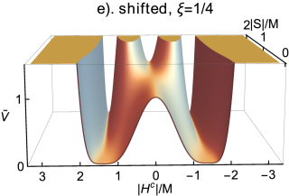

In Fig. 1, the standard HI case with is reproduced in plot (a). In this case, , is the only inflationary valley available. It evolves at into a single pair of global SUSY minima with vev . For , in addition to the standard track at , two shifted local minima appear at for . In plot (b) for , the shifted tracks lie higher than the standard track. Following Ref. Jeannerot:2000sv , in order to have suitable initial conditions for realizing inflation along the shifted tracks, we assume . The normalized scalar potential is shown in plots (c)-(e) for some realistic values of , namely for , , and . In the last plot (f) with , we obtain , since the SUSY minimum requires complex values of , . So for our analysis, it is appropriate to keep within the interval .
As the inflaton slowly rolls down the inflationary valley and enters the waterfall regime at , inflation ends due to fast rolling and the system starts oscillating about a vacuum at . Note that in the direction there are actually two pairs of vacua at [see Eq. (21c)]
| (22) |
However, the path leading to appears before the one leading to , as explained in Ref. Jeannerot:2000sv . The necessary slope for realizing inflation in the valley with , , is generated by the inclusion of the one-loop radiative corrections, the SUGRA corrections, and the soft SUSY breaking terms. The one-loop radiative corrections , arising as a result of SUSY breaking on the inflationary path, are calculated using the Coleman-Weinberg formula Coleman;1973 :
| (23) |
where and are the fermion number and squared mass of the ith state. The function is given by
| (24) |
with , and is defined in terms of the canonically normalized real inflaton field as with . The function exhibits the contribution of the term in the superpotential , and for , is expected to play an important role in the predictions of inflationary observables. The renormalization scale is set equal to , the field value at the pivot scale Akrami:2018odb .
The soft SUSY breaking terms are added in the inflationary potential as:
| (25) |
where is the complex coefficient of the trilinear soft-SUSY-breaking terms.
Trying to reconcile supergravity and cosmic inflation, one runs into the so-called problem which arises as the effective inflationary potential is quite steep. This leads to large inflaton masses on the order of the Hubble parameter and thus the slow-roll conditions are violated. In hybrid inflationary scenarios, the supergravity corrections can easily be brought under control Lazarides:1996dv ; Panagiotakopoulos:1997ej ; Dvali:1997uq ; Lazarides:1998zf ; Dimopoulos:2011ym . Another potential problem is the appearance of anti-de Sitter vacua. However, in hybrid inflation models, these vacua may be lifted – for examples see Refs. Haba:2005ux ; Wu:2016fzp .
The -term SUGRA scalar potential is evaluated using,
| (26) |
where and
| (27) |
The Kähler potential is expanded in inverse powers of :
| (28) |
where the minimal canonical Kähler potential is given by
| (29) |
The inflationary potential along the D-flat direction with , stabilized along the direction, and incorporating the SUGRA corrections Linde:1997sj , the radiative corrections Dvali:1994ms , and the soft-SUSY-breaking terms Senoguz:2004vu ; Rehman:2009nq , is given by
| (30) |
Here , , and are the coefficients of the constant, quadratic, and quartic SUGRA terms, respectively, and are defined in terms of as
| (31) |
where Civiletti:2011qg . For the inflationary potential along the D-flat and direction, the independently varying parameters , , and for the nonminimal case are the same as the ones given in Ref. Civiletti:2011qg . Our choice for these parameters will be shown in the relevant sections. The parameter depends on as follows:
| (32) |
Assuming negligible variation in , with , the scalar spectral index is expected to lie within the experimental range Rehman:2009nq ; Civiletti:2011qg . This could also be achieved by taking an intermediate-scale, negative soft mass-squared term for the inflaton Rehman:2009yj . But with the nonminimal terms in the Kähler potential, one can also obtain the central value of with TeV-scale soft masses even for BasteroGil:2006cm ; urRehman:2006hu . The variation in with general initial condition has been studied in Refs. Senoguz:2004vu ; urRehman:2006hu ; Buchmuller:2014epa .
The slow-roll parameters are defined by
| (33) |
where the primes denote derivatives with respect to . The scalar spectral index , the tensor-to-scalar ratio , the running of the scalar spectral index , and the scalar power spectrum amplitude , to leading order in the slow-roll approximation, are as follows:
| (34a) | ||||
| (34b) | ||||
| (34c) | ||||
| (34d) | ||||
where and denotes the value of at the pivot scale Akrami:2018odb . For the numerical estimation of the inflationary predictions, these relations are used up to second order in the slow-roll parameters.
Assuming a standard thermal history, the number of -folds between the horizon exit of the pivot scale and the end of inflation is
| (35) | ||||
The reheat temperature is approximated by
| (36) |
where for MSSM and is the inflaton decay width. From the -term coupling in Eq. (15), we see that the inflaton can decay into a pair of Higgsinos , with a decay width
| (37) |
where
| (38) |
is the inflaton mass Jeannerot:2000sv . The reheat temperature, the inflaton decay width, and the inflaton mass defined above in Eqs. (36)-(38) are used together with Eq. (35) in order to derive the numerical predictions for the present inflationary scenario.
IV -hybrid inflation with minimal Kähler potential
The inflationary potential corresponding to the minimal Kähler potential in Eq. (29) is easily transcribed from Eq. (III) as follows:
| (39) |
since, in this case, , and, thus, the coefficients , .

In Fig. 2, we plot the gravitino mass versus the reheat temperature as constrained by inflation. The solid-magenta, dashed-blue, dot-dashed-green curves correspond to respectively for the minimal Kähler potential with the conditions , , , and . The lower bound on the reheat temperature GeV is obtained for a gravitino mass with a fine-tuning of the difference .
Following the same line of argument as in Refs. Okada:2015vka ; Rehman:2017gkm , the shifted HI with minimal is analyzed for the following three cases:
-
1.
stable gravitino LSP;
-
2.
unstable long-lived gravitino with ;
-
3.
unstable short-lived gravitino with .
The relic gravitino abundance, in the case of a stable gravitino LSP, is given Bolz:2000fu by
| (40) |
where is the gluino mass. We require that does not exceed the observed DM relic abundance, that is Akrami:2018odb . Using Eq. (40), we then plot in Fig. 2 the resulting upper limit on the gluino mass . The point where and the upper bound on coincide, for the central value of (i.e. ), lies at GeV and GeV as shown by the intersection of the corresponding curves. Our assumption for a gravitino LSP holds for values below this intersection point, that is for GeV, GeV. However, the maximum value of the gluino mass in this region is GeV which is lower than the lower bound on the gluino mass TeV from the search for supersymmetry at the LHC Tanabashi:2018oca . Consequently, we run into inconsistency and the case of a stable gravitino LSP with a minimal Kähler potential is ruled out.
In the second case, the long-lived unstable gravitino will decay after big bang nucleosynthesis (BBN), and so one has to take into account the BBN bounds on the reheat temperature which are the following Khlopov:1993ye ; Kawasaki:2004qu ; Kawasaki:2017bqm :
| (41) |
The bounds on the reheat temperature from the inflationary constraints for gravitino masses are and respectively (see Fig. 2). These are clearly inconsistent with the above mentioned BBN bounds, and so the unstable long-lived gravitino scenario is not viable.
Lastly, for the unstable short-lived gravitino case, we compute the LSP lightest neutralino () density produced by the gravitino decay and constrain it to be smaller than the observed DM relic density. For reheat temperature with (see Fig. 2), the resulting bound on the neutralino mass comes out to be inconsistent with the lower limit set on this mass in Ref. Hooper:2002nq . To circumvent this, the LSP neutralino is assumed to be in thermal equilibrium during gravitino decay, whereby the neutralino abundance is independent of the gravitino yield. For an unstable gravitino, the lifetime is (see Fig. 1 of Ref. Kawasaki:2008qe )
| (42) |
Now for a typical value of the neutralino freeze-out temperature, , the gravitino lifetime is estimated to be
| (43) |
Comparing Eq. (42) and Eq. (43), we obtain a bound on ,
| (44) |
Thus, minimal shifted HI conforms with the conclusion of the standard case Okada:2015vka ; Rehman:2017gkm by requiring split-SUSY with an intermediate-scale gravitino mass and reheat temperature (see Fig. 2). To check whether the shifted HI scenario is also compatible with low reheat temperature (i.e. Khlopov:1984pf ) and TeV-scale soft SUSY breaking, we employ nonminimal Kähler potential in the next section.
V -hybrid inflation with nonminimal Kähler potential
The nonminimal Kähler potential used in the following analysis is
| (45) |
which includes only the nonminimal couplings of interest and . (For a somewhat different approach to -hybrid inflation with nonminimal , see Ref. Okada:2017rbf ). Thus, for the nonminimal scenario we take and in Eq. (31) Civiletti:2011qg . Using these values the potential of the system can easily be read off from Eq. (III).
It is worth noting that with the nonminimal Kähler potential we can realize the central value of with TeV-scale soft masses even for BasteroGil:2006cm ; urRehman:2006hu . Our study is conducted in two parts, described separately in the following subsections, first with and then by allowing to be nonzero. The appearance of a negative mass term with a single nonminimal coupling in the potential in Eq. (III) is expected to lead to red-tilted inflation with low reheat temperature, as for standard HI (see Ref. Rehman:2017gkm ). Furthermore for nonzero , the possible larger solutions leading to observable gravity waves are also anticipated. These expectations along with the impact of an additional parameter on inflationary predictions are discussed below.
V.1 Low reheat temperature and the gravitino problem


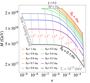
Incorporating the inflationary constraints and the nonminimal in Eq. (45) with , we summarize some of the results depicting the main features of nonminimal shifted HI in Figs. 3 – 5. From these figures it is clear that with low reheat temperature we can obtain a higher mass scale ranging from to the string scale . The reheat temperature is lowered by nearly half an order of magnitude in the shifted HI as compared to the standard HI (see Fig. 2 of Ref. Rehman:2017gkm ), as can be seen from Fig. 3. Also, it is not surprising that around the system is oblivious to the gravitino mass, since the contribution of the linear term becomes less important compared with the SUGRA or radiative corrections BasteroGil:2006cm . The interesting new feature is due to the presence of another parameter , whose effect is to increase the range of mass scale . For a particular value of , say , and , a wider range of exists, corresponding to in the range (see Fig. 4). So there is an order of magnitude increase in the spread of , compared with standard HI, where the maximum value is corresponding to the lowest reheat temperature , with gravitino of mass Rehman:2017gkm . This maximum value has now increased to with in the range . Also, the lower plot of Fig. 4 shows the variation of with respect to the tensor-to-scalar ratio with , which is experimentally inaccessible in the foreseeable future Andre:2013afa ; Matsumura:2013aja ; Kogut:2011 ; Finelli:2016cyd .
As Fig. 5 shows, the running of the scalar spectral index also turns out to be small in the present scenario, namely , which is a common feature of small field models. The nonminimal Kähler coupling remains constant in the low reheat temperature range as can be seen from the lower plot of Fig. 5, since the radiative and the quartic-SUGRA corrections can be neglected in this regime. The scalar spectral index in the low reheat temperature region is King:1997ia , and so for the central value of the scalar spectral index , one obtains , as exemplified by Fig. 5. To explore larger values of , we will make use of the freedom provided by the second nonrenormalizable coupling in the next section. Note that the number of e-folds in Eq. (35) generally ranges between about 47 and 56.
Proceeding next to the role of the gravitino in cosmology, one can read off the lower bounds on the reheat temperature from Fig. 3. Since, at low reheat temperatures, inflation occurs near the waterfall region (with close to 1), we devised a criterion by allowing only fine-tuning on the difference . This yields
| (46) |
For the first scenario with the gravitino being the LSP in shifted HI with nonminimal Kähler potential, the upper bounds on the reheat temperature obtained in Ref. Rehman:2017gkm (see Fig. 3 and Eq. (30) in this reference) are respectively. These upper bounds on are consistent with the lower bounds in Eq. (46), and so the scenario with the gravitino as LSP can be consistently realized in the nonminimal Kähler case.
For the second possibility, namely an unstable long-lived gravitino (with ), comparison of Eqs. (IV) and Eq. (46) reveals that an gravitino is marginally ruled out but a gravitino lies comfortably within the BBN bounds.
For the third scenario of a short-lived gravitino (for instance with mass ), the gravitino decays before BBN, and so the BBN bounds on the reheat temperature no longer apply. The gravitino decays into the LSP neutralino . We find that the resulting neutralino abundance is given by
| (47) |
where the gravitino yield
| (48) |
is acceptable over the range Kawasaki:2008qe . The LSP (lightest neutralino) density produced by the gravitino decay should not exceed the observed DM relic density Akrami:2018odb . The resulting bound on the lightest neutralino mass
| (49) |
turns out to be less restrictive than the corresponding bound from the abundance of the lightest neutralino from the gravitino decay in the case of standard HI. Indeed, the non-LSP gravitino with is acceptable in a larger domain, namely . There is nearly an order of magnitude decrease in the acceptable lower reheat temperature as compared with the standard HI. Note that the lower limit on the neutralino mass, , is obtained in Ref. Hooper:2002nq by employing a minimal set of theoretical assumptions. In conclusion the shifted HI is successful with and low reheat temperatures.
V.2 Large solutions or observable gravity waves


The canonical measure of primordial gravity waves is the tensor-to-scalar ratio and the next-generation experiments are gearing up to measure it. One of the highlights of PRISM Andre:2013afa is to detect inflationary gravity waves with as low as and a major goal of LiteBIRD Matsumura:2013aja is to attain a measurement of within an uncertainty of . Future missions include PIXIE Kogut:2011 , which aims to measure at standard deviations, and CORE Finelli:2016cyd , which forecasts to lower the detection limit for the tensor-to-scalar ratio down to the level.
As seen in previous sections, with , the tensor-to-scalar ratio remains in the undetectable range . It is therefore instructive to explore our model further to look for large- solutions, which, as it turns out, yield ’s in the range. To achieve this, we employ nonzero in addition to a nonzero , and the results are presented in Figs. 6–9, for a range of values of the field at horizon crossing of the pivot scale . In addition, the variation of the parameter is also depicted in these figures by plotting results with and .


The curves corresponding to field values close to are terminated since, at some point, either the nonminimal coupling takes unnatural values (see Fig. 9) or reaches . Indeed, for , the coupling can exceed the bound of 10 on curves with and, for , the mass scale can exceed on curves with . We see that the mass scale is not independent of . In fact, as increases from to , the mass scale also increases (this is observed in the case as well). The curves are terminated at their left end due to the fine-tuning bound that we used in the numerical work. The solid-gray lines in Figs. 6–8 are the constant reheat temperature lines, starting from the upper cutoff at GeV and going down to values as low as .
The upper bound on the tensor-to-scalar ratio , as can be read off from Fig. 6, is for the choice of the field and for . Fig. 6 also shows that from the requirement that the reheat temperature for circumventing the gravitino problem. The running of the scalar spectral index remains small namely , as shown in Fig. 7. The variation of the mass scale with is shown in Fig. 8, where we find values of the parameter up to for large values of (). The respective variation in the coupling constants and is shown in Fig. 9. They remain acceptably small and well within the bound , for natural values of or less.
| 1 | 2 | 3 | 4 | 5 | 6 | |
| 0 | 0.006 | 0.017 | -0.02 | 0.19 | 0.19 | |
| 0 | 0 | 0 | 1.3 | 0.15 | 0.84 | |
| 0.125 | 0.125 | 0.125 | 0.125 | 0.2 | ||
| (GeV) | ||||||
| 0.04 | 0.005 | 0.006 | 0.1 | 1 | 0.1 | |
| (GeV) | ||||||
| (GeV) |
Although the plots presented in Figs. 6–9 are for gravitino mass , the curves, for these larger solutions, are independent of the gravitino mass and are valid for a gravitino mass range .
Benchmark points for minimal and nonminimal Kähler potential, for fixed values of , , and , are given in Table 2 along with the corresponding values of the couplings , , , and the tensor-to-scalar ratio , the running of the spectral index , the mass scale , and the reheat temperature . A viable scenario for the minimal case is shown in column 1 with an unstable gravitino being the next-to-LSP (NLSP) and decaying into the neutralino LSP before its freeze-out. Column 2 shows that the maximum value of for is , which is too small to be observable. Column 3 shows that reheat temperatures GeV can be easily obtained for mass scales around the GUT scale. At large field values , the results are shown in columns 4-6 and are more or less independent of the gravitino mass.
VI Conclusion
We have implemented a version of SUSY hybrid inflation in , a well motivated extension of the SM. This maximal subgroup of Spin contains electric charge quantization and arises in a variety of string theory constructions. The MSSM term arises, following Dvali, Lazarides, and Shafi, from the coupling of the electroweak doublets to a gauge singlet superfield playing an essential role in inflation, which takes place along a shifted flat direction. The scheme with minimal Kähler potential leads to an intermediate scale gravitino mass with the gravitino decaying before the freeze out of the LSP neutralinos and with reheat temperature Okada:2015vka . This points towards split SUSY. In the nonminimal Kähler case, we have realized successful inflation with reheat temperatures as low as . This is favorable for the resolution of the gravitino problem and compatible with a stable LSP and low-scale (TeV) SUSY. Compared with standard hybrid inflation Rehman:2017gkm , the reheat temperature is lowered by half an order of magnitude and, due to the additional parameter , an order of magnitude increase in the spread of is seen. We have discussed how primordial monopoles are inflated away and provided a framework that predicts the presence of primordial gravity waves with the tensor-to-scalar ratio in the observable range (). This is realized with the mass scale M scale approaching values that are comparable to the string scale () and a gravitino mass lying in the range. It is worth noting that the inflaton field values do not exceed the Planck scale, which may be an additional desirable feature in view of the swampland conjectures Vafa:2005ui ; Ooguri:2006in . For a recent discussion and additional references see Ref. Vafa:2019evj .
Acknowledgments
The work of G.L. and Q.S. was supported by the Hellenic Foundation for Research and Innovation (H.F.R.I.) under the “First call for H.F.R.I. research projects to support faculty members and researchers and the procurement of high-cost research equipment grant” (Project Number:2251).
References
- (1) G.R. Dvali, Q. Shafi, and R.K. Schaefer, “Large scale structure and supersymmetric Inflation without fine-tuning,” Phys. Rev. Lett. 73, 1886 (1994) [hep-ph/9406319].
- (2) E.J. Copeland, A.R. Liddle, D.H. Lyth, E.D. Stewart, and D. Wands, “False vacuum inflation with Einstein gravity,” Phys. Rev. D 49, 6410 (1994) [astro-ph/9401011].
- (3) V.N. Senoguz and Q. Shafi, “Reheat temperature in supersymmetric hybrid inflation models,” Phys. Rev. D 71, 043514 (2005) [hep-ph/0412102].
- (4) M.U. Rehman, Q. Shafi, and J.R. Wickman, “Supersymmetric hybrid inflation redux,” Phys. Lett. B 683, 191 (2010) [hep-ph/0908.3896].
- (5) C. Pallis and Q. Shafi, “Update on minimal supersymmetric hybrid inflation in light of PLANCK,” Phys. Lett. B 725, 327 (2013) [hep-ph/1304.5202].
- (6) W. Buchmüller, V. Domcke, K. Kamada, and K. Schmitz, “Hybrid inflation in the complex plane,” J. Cosmol. Astropart. Phys. 07, 054 (2014) [astro-ph.CO/1404.1832].
- (7) Y. Akrami et al. [Planck Collaboration], “Planck 2018 results. X. Constraints on inflation,” astro-ph.CO/1807.06211.
- (8) M. Bastero-Gil, S.F. King, and Q. Shafi, “Supersymmetric hybrid inflation with nonminimal Kähler potential,” Phys. Lett. B 651, 345 (2007) [hep-ph/0604198].
- (9) M.U. Rehman, V.N. Senoguz, and Q. Shafi, “Supersymmetric and smooth hybrid inflation in the light of WMAP3,” Phys. Rev. D 75, 043522 (2007) [hep-ph/0612023].
- (10) M.U. Rehman, Q. Shafi, and J.R. Wickman, “Observable gravity waves from supersymmetric hybrid inflation II,” Phys. Rev. D 83, 067304 (2011) [astro-ph.CO/1012.0309].
- (11) M. Civiletti, C. Pallis, and Q. Shafi, “Upper bound on the tensor-to-scalar ratio in GUT-scale supersymmetric hybrid inflation,” Phys. Lett. B 733, 276 (2014) [hep-ph/1402.6254].
- (12) R. Jeannerot, S. Khalil, G. Lazarides, and Q. Shafi, “Inflation and monopoles in supersymmetric ,” J. High Energy Phys. 10, 012 (2000) [hep-ph/0002151].
- (13) G. Lazarides, “Supersymmetric hybrid inflation,” NATO Sci. Ser. II 34, 399 (2001) [hep-ph/0011130]; R. Jeannerot, S. Khalil, and G. Lazarides, “Monopole problem and extensions of supersymmetric hybrid inflation,” Proc. of CICHEP 2001, 254 (2001) [hep-ph/0106035].
- (14) J.C. Pati and A. Salam, “Lepton number as the fourth color,” Phys. Rev. D 10, 275 (1974), Erratum: Phys. Rev. D 11, 703 (1975).
- (15) S.F. King and Q. Shafi, “Minimal supersymmetric ,” Phys. Lett. B 422, 135 (1998) [hep-ph/9711288].
- (16) G.R. Dvali, G. Lazarides, and Q. Shafi, “ problem and hybrid inflation in supersymmetric ,” Phys. Lett. B 424, 259 (1998) [hep-ph/9710314].
- (17) M.Y. Khlopov and A.D. Linde, “Is it easy to save the gravitino?,” Phys. Lett. B 138, 265 (1984); J.R. Ellis, J.E. Kim, and D.V. Nanopoulos, “Cosmological gravitino regeneration and decay,” Phys. Lett. B 145, 181 (1984).
- (18) G. Lazarides and N. D. Vlachos, “Atmospheric neutrino anomaly and supersymmetric inflation,” Phys. Lett. B 441, 46 (1998) [hep-ph/9807253].
- (19) N. Okada and Q. Shafi, “-term hybrid inflation and split supersymmetry,” Phys. Lett. B 775, 348 (2017) [hep-ph/1506.01410].
- (20) Q. Shafi and Z. Tavartkiladze, “Neutrino oscillations and other key issues in supersymmetric ,” Nucl. Phys. B 549, 3 (1999) [hep-ph/9811282].
- (21) G. Lazarides and C. Panagiotakopoulos, “MSSM from SUSY trinification,” Phys. Lett. B 336, 190 (1994) [hep-ph/9403317]; G. Dvali and Q. Shafi, “Gauge hierarchy, Planck scale corrections and the origin of GUT scale in supersymmetric ,” Phys. Lett. B 339, 241 (1994) [hep-ph/9404334].
- (22) M.U. Rehman, Q. Shafi, and F.K. Vardag, “-hybrid inflation with low reheat temperature and observable gravity waves,” Phys. Rev. D 96, 063527 (2017) [hep-ph/1705.03693].
- (23) A.H. Chamseddine, R.L. Arnowitt, and P. Nath, “Locally supersymmetric grand unification,” Phys. Rev. Lett. 49, 970 (1982).
- (24) A.D. Linde and A. Riotto, “Hybrid inflation in supergravity,” Phys. Rev. D 56, R1841 (1997) [hep-ph/9703209].
- (25) B. Kyae and Q. Shafi, “Inflation with realistic supersymmetric SO(10),” Phys. Rev. D 72, 063515 (2005) [hep-ph/0504044].
- (26) S. Coleman and E. Weinberg, “Radiative corrections as the origin of spontaneous symmetry breaking,” Phys. Rev. D 7, 1888 (1973).
- (27) G. Lazarides, R. K. Schaefer, and Q. Shafi, “Supersymmetric inflation with constraints on superheavy neutrino masses,” Phys. Rev. D 56, 1324 (1997) [hep-ph/9608256].
- (28) C. Panagiotakopoulos, “Hybrid inflation with quasicanonical supergravity,” Phys. Lett. B 402, 257 (1997) [hep-ph/9703443].
- (29) G. Lazarides and N. Tetradis, “Two stage inflation in supergravity,” Phys. Rev. D 58, 123502 (1998) [hep-ph/9802242].
- (30) K. Dimopoulos, G. Lazarides, and J. M. Wagstaff, “Eliminating the -problem in SUGRA Hybrid Inflation with Vector Backreaction,” JCAP 02, 018 (2012) [astro-ph.CO/1111.1929].
- (31) N. Haba and N. Okada, “Structure of split supersymmetry and simple models,” Prog. Theor. Phys. 114, 1057 (2006) [hep-ph/0502213].
- (32) L. Wu, S. Hu, and T. Li, “No-Scale -Term Hybrid Inflation,” Eur. Phys. J. C 77 no.3, 168 (2017) [hep-ph/1605.00735].
- (33) M. Civiletti, M.U. Rehman, Q. Shafi, and J.R. Wickman, “Red spectral tilt and observable gravity waves in shifted hybrid inflation,” Phys. Rev. D 84, 103505 (2011) [astro-ph.CO/1104.4143].
- (34) M.U. Rehman, Q. Shafi, and J.R. Wickman, “Minimal supersymmetric hybrid inflation, flipped SU(5) and proton decay,” Phys. Lett. B 688, 75 (2010) [hep-ph/0912.4737].
- (35) M. Bolz, A. Brandenburg, and W. Buchmuller, Thermal production of gravitinos, Nucl. Phys. B606, 518 (2001); Nucl. Phys. B790, 336(E) (2008) [hep-ph/0012052].
- (36) M. Tanabashi et al. [Particle Data Group], “Review of Particle Physics,” Phys. Rev. D 98 no.3, 030001(2018).
- (37) M. Khlopov, Y. Levitan, E. Sedelnikov, and I. Sobol, “Nonequilibrium cosmological nucleosynthesis of light elements: Calculations by the Monte Carlo method,” Phys. Atom. Nucl. 57, 1393 (1994).
- (38) M. Kawasaki, K. Kohri, and T. Moroi, “Big-Bang nucleosynthesis and hadronic decay of long-lived massive particles,” Phys. Rev. D 71, 083502 (2005) [astro-ph/0408426].
- (39) M. Kawasaki, K. Kohri, T. Moroi, and Y. Takaesu, “Revisiting big-bang nucleosynthesis constraints on long-lived decaying particles,” Phys. Rev. D 97, 023502 (2018) [hep-ph/1709.01211].
- (40) D. Hooper and T. Plehn, “Supersymmetric dark matter: How light can the LSP be?,” Phys. Lett. B 562, 18 (2003) [hep-ph/0212226].
- (41) M. Kawasaki, K. Kohri, T. Moroi, and A. Yotsuyanagi, “Big-bang nucleosynthesis and gravitino,” Phys. Rev. D 78, 065011 (2008) [hep-ph/0804.3745].
- (42) M. Khlopov and A.D. Linde, “Is it easy to save the gravitino?,” Phys. Lett. B 138, 265 (1984).
- (43) N. Okada and Q. Shafi; “Gravity waves and gravitino dark matter in -hybrid inflation,” Phys. Lett. B 787, 141 (2018) [hep-ph/1709.04610].
- (44) P. Andre et al. (PRISM Collaboration), “PRISM (Polarized Radiation Imaging and Spectroscopy Mission): A white paper on the ultimate polarimetric spectro-imaging of the microwave and far-infrared sky,” astro-ph.CO/1306.2259.
- (45) T. Matsumura et al., “Mission design of LiteBIRD,” J. Low. Temp. Phys. 176, 733 (2014) [astro-ph.CO/1311.2847].
- (46) A. Kogut et al., “The Primordial Inflation Explorer (PIXIE): a nulling polarimeter for cosmic microwave background observations,” J. Cosmol. Astropart. Phys. 07, 025 (2011) [astro-ph.CO/1105.2044].
- (47) F. Finelli et al. [CORE Collaboration], “Exploring cosmic origins with CORE: Inflation,” JCAP 04, 016 (2018) [astro-ph.CO/1612.08270].
- (48) C. Vafa, “The string landscape and the swampland,” hep-th/0509212.
- (49) H. Ooguri and C. Vafa, “On the geometry of the string landscape and the swampland,” Nucl. Phys. B 766, 21 (2007) [hep-th/0605264].
- (50) C. Vafa, “Cosmic Predictions from the String Swampland,” APS Physics 12, 115 (2019).