SHIFT Planner: Speedy Hybrid Iterative Field and Segmented Trajectory Optimization with IKD-tree for Uniform Lightweight Coverage
Abstract
Efficient and uniform coverage in complex and dynamic environments is crucial for autonomous robots performing tasks such as cleaning, inspection, and agricultural operations. However, existing methods often focus on minimizing traversal time or path length, neglecting the importance of uniform coverage and adaptability to environmental attributes. This paper introduces a comprehensive planning and navigation framework that addresses these limitations by integrating semantic mapping, adaptive coverage planning, dynamic obstacle avoidance, and precise trajectory tracking.
Our framework begins by generating Panoptic Occupancy local semantic maps and accurate localization information from data aligned between a monocular camera, IMU, and GPS. This information is combined with input terrain point clouds or preloaded terrain information to initialize the planning process. We propose the Radiant Field-Informed Coverage Planning (RFICP) algorithm, which utilizes a diffusion field model to dynamically adjust the robot’s coverage trajectory and speed based on environmental attributes such as dirtiness or dryness. By modeling the spatial influence of the robot’s actions using a Gaussian field, RFICP ensures a speed-optimized, uniform coverage trajectory while adapting to varying environmental conditions.
When dynamic obstacles are encountered along the planned path, we introduce a rapid path optimization method called Incremental IKD-tree Sliding Window Optimization (IKD-SWOpt) for obstacle avoidance. IKD-SWOpt continuously monitors the path within a circular detection window—referred to as the Circular Judgment and Assessment Module—to identify regions that violate the defined path cost function. These segments are incorporated into an Adaptive Sliding Window for localized optimization, iteratively refining the trajectory until a collision-free path is achieved. This approach enhances real-time performance and computational efficiency by activating the optimization framework only when necessary.
Extensive experiments conducted with drones and robotic vacuum cleaners in complex real-world environments validate the effectiveness of our approach. The proposed framework demonstrates superior coverage performance and adaptability compared to existing methods, achieving efficient, uniform, and obstacle-aware trajectories suitable for autonomous systems operating in dynamic environments.
Index Terms:
Autonomous robots, Coverage planning, Radiant Field-Informed Coverage Planning (RFICP), Incremental IKD-tree Sliding Window Optimization (IKD-SWOpt), Dynamic obstacle avoidance, Semantic mapping.I Introduction
With the large-scale integration of cleaning robots into human life, there is an increasing demand for efficient algorithm architectures that ensure uniform scene traversal and coverage. For tasks requiring uniform path coverage—such as surface wiping by cleaning robots, uniform pesticide spraying by agricultural drones, and room cleaning by robotic vacuum cleaners—existing methods often focus solely on shortest path traversal and time optimization. They overlook the need to model spatial coverage and environmental attributes, such as adjusting the robot’s behavior based on detected dirtiness or dryness levels.
In practical applications, robots not only need to traverse the entire workspace but also need to model environmental characteristics and adjust their actions accordingly. For example, a robotic vacuum cleaner should slow down and clean more thoroughly upon detecting dirtier areas. Similarly, a drone spraying pesticides should linger longer over drier crops to achieve the desired coverage.
This paper addresses these challenges by proposing SHIFT Planner, a novel planning and navigation framework that:
-
•
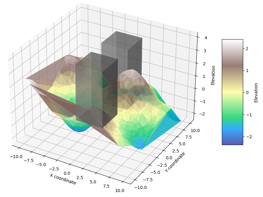
Extends uniform coverage planning from 2D to 3D using a differential geometry-based contour surface extraction method applied to real terrain point clouds collected from sensors.
-
•
Eliminates the need for region decomposition by directly planning on surface landmarks.
-
•
Introduces a dynamic trajectory planning algorithm that activates local optimization only when necessary, reducing computational overhead.
-
•
Incorporates environmental attribute modeling using Gaussian fields to adjust robot behavior dynamically.
-
•
Integrates IKD-tree for lightweight mapping to enhance real-time performance.
Our contributions are validated through extensive experiments with drones and robotic vacuum cleaners in simulated and real-world environments, demonstrating the framework’s efficacy in complex coverage tasks. The proposed SHIFT Planner outperforms existing methods in terms of coverage uniformity, adaptability to environmental attributes, and computational efficiency.
The code and additional resources are open-sourced and available at: https://fanzexuan.github.io/shiftplanner/
II Related Work
II-A Coverage Path Planning in Robotics
Coverage Path Planning (CPP) is a fundamental problem in robotics, aiming to determine a path that allows a robot to cover an entire area or volume [1, 2]. Traditional CPP methods include:
-
•
Cell Decomposition Methods: Such as Boustrophedon Cellular Decomposition (BCD) [3], which divide the workspace into simple cells and plan coverage paths within each cell.
-
•
Grid-Based Methods: Utilize occupancy grids to represent the environment, planning paths that ensure each grid cell is visited.
-
•
Randomized Methods: Include algorithms like Rapidly-exploring Random Trees (RRT) [4], which are less suitable for uniform coverage due to their stochastic nature.
II-B Limitations of Existing Methods
Coverage Path Planning in complex 3D environments has been extensively studied, leading to the development of various methodologies. Notable among these are:
II-B1 Hierarchical Coverage Path Planning
Cao et al. [5] introduced a hierarchical framework that decomposes complex 3D spaces into manageable subregions, facilitating efficient coverage. However, this approach primarily focuses on spatial decomposition and may not adequately account for dynamic environmental attributes such as varying levels of dirtiness or dryness, which are crucial for adaptive coverage tasks.
II-B2 Sampling-Based View Planning
Jing et al. [6] proposed a sampling-based view planning algorithm for UAVs to acquire visual geometric information of target objects. While effective in viewpoint selection, this method may not fully integrate real-time sensor data for terrain representation, potentially limiting its responsiveness to dynamic environmental changes.
II-B3 Skeleton-Guided Planning Framework
Feng et al. [7] developed FC-Planner, a skeleton-guided planning framework that decomposes the scene into simple subspaces using skeleton-based space decomposition. Despite its computational efficiency, it may not sufficiently model environmental attributes like dirtiness or dryness, which are essential for tasks requiring adaptive coverage based on such factors.
II-B4 Artificial Potential Field-Based Multi-Robot Online CPP
The APF-CPP approach employs artificial potential fields to facilitate online coverage path planning for multiple robots in dynamic environments. However, it may encounter challenges related to local minima and might not effectively integrate preloaded terrain data or previously established semantic maps, which are vital for informed planning processes.
While existing methods have advanced obstacle avoidance and path optimization, they often fall short in addressing certain critical challenges in practical coverage tasks, such as:
-
•
Uniform Coverage: Ensuring equal attention across the entire workspace without overly focusing on shortest path considerations.
-
•
Environmental Attribute Modeling: Dynamically adjusting robot behavior based on spatial properties like dirtiness or dryness, ensuring coverage planning adapts to real-world conditions.
-
•
3D Environment Adaptability: Extending traditional 2D planning methods to complex 3D surfaces while maintaining efficiency and uniformity in the coverage.
-
•
Real Sensor Data Integration: Utilizing actual terrain data from various sensors, such as monocular cameras, IMUs, GPS, and terrain point clouds, to accurately represent the environment.
Moreover, existing optimization methods based on ESDF (Euclidean Signed Distance Fields) mapping introduce significant memory overhead and may compromise precision, limiting their effectiveness in large or complex scenarios. These methods also tend to focus on optimizing kinematic properties such as velocity, acceleration, jerk, and snap. However, they often lack direct integration with specific planning tasks, leading to a gap between path smoothness and actual task efficiency.
In this paper, we propose a trajectory planning approach that integrates these aspects, specifically addressing the needs of real-world cleaning or coverage tasks. By coupling the optimization process with the requirements of the practical planning task, we ensure efficient and task-relevant trajectory generation that balances uniform coverage with kinematic optimality.
III System Overview
The proposed SHIFT Planner framework integrates multiple key components to achieve adaptive, efficient, and robust path planning and semantic mapping for autonomous systems in dynamic environments. The main modules are as follows:
-
1.
Input Data:
-
•
Sensor Inputs: Includes data from a monocular camera, Inertial Measurement Unit (IMU), and odometer.
-
•
Terrain Point Cloud: Generated using LiDAR and other sensors to provide detailed environmental context.
-
•
Initial Semantic Map: Created through semantic segmentation of sensor data for high-level scene understanding.
-
•
-
2.
Global Mapping:
-
•
Scan2Map Module: Processes raw sensor data into a series of point clouds.
-
•
Global Map Fusion: Aggregates sequential point clouds into a coherent and unified global map.
-
•
-
3.
Semantic Mapping:
-
•
Panoptic Occupancy Segmentation: Integrates instance and semantic segmentation for comprehensive and accurate scene analysis, facilitating context-aware decision-making.
-
•
-
4.
Path Planning:
-
•
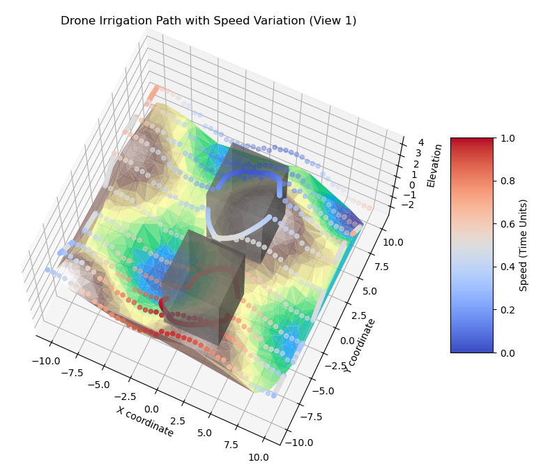
Radiant Field-Informed Coverage Planning (RFICP): Generates coverage trajectories while accounting for environmental attributes to ensure uniform and efficient area exploration.
-
•
Trajectory Speed Reallocation: Dynamically adjusts robot velocity to accommodate varying terrain conditions.
-
•
-
5.
Local Mapping:
-
•
IKD-tree Updating: Efficiently maintains an up-to-date local map in real-time.
-
•
Local Map Fusion: Integrates local point clouds into the global map for continuity and detail.
-
•
Visual-Inertial Odometry: Provides precise localization by fusing visual and inertial data.
-
•
Pose Graph Optimization: Reduces drift and enhances trajectory accuracy over extended operation periods.
-
•
Local Optimization and Collision Checking: Refines trajectories to ensure safety and obstacle avoidance.
-
•
IKD-SWOpt: A sliding window optimization algorithm leveraging an IKD-tree structure for incremental updates.
-
•
-
6.
Adaptation Detection:
-
•
Circular Judgment and Assessment Module: Monitors environmental changes to detect dynamic obstacles or evolving terrain.
-
•
Adaptive Sliding Window: Adjusts optimization parameters dynamically to respond to environmental variations.
-
•
-
7.
Tracking:
-
•
Trajectory Server: Manages and stores trajectory segments generated during planning.
-
•
Tracking Controller: Ensures accurate execution of planned and optimized paths.
-
•
The system architecture is visually depicted in Figure 1.
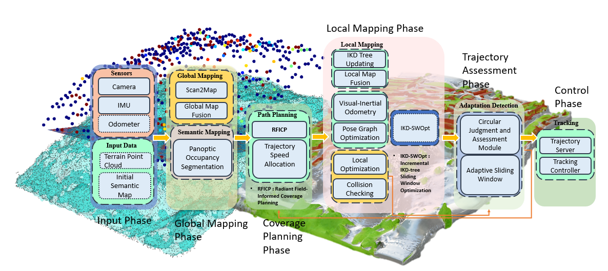
This framework combines semantic mapping, path planning, and obstacle avoidance to enhance autonomous navigation. Using monocular camera and IMU data, the system constructs a Panoptic Occupancy local semantic map and derives localization information. Preloaded terrain data or prior semantic maps are optionally used to initialize the planning process. Based on these inputs, the RFICP algorithm computes efficient coverage trajectories, optimizing both path coverage and velocity profiles.
In dynamic environments, when obstacles disrupt the planned path, the IKD-SWOpt algorithm enables rapid path adjustments. Within a Circular Judgment and Assessment Module, the algorithm identifies trajectory segments with cost violations and integrates them into an Adaptive Sliding Window for iterative optimization. This process ensures real-time collision-free path generation and refinement.
Finally, the Tracking Controller module ensures precise execution of the optimized trajectory, maintaining adherence to the planned path. The integrated approach effectively addresses challenges in dynamic and cluttered environments, demonstrating adaptability, efficiency, and robustness in autonomous trajectory planning.
IV Methodology
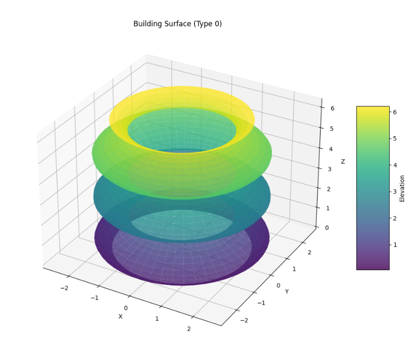
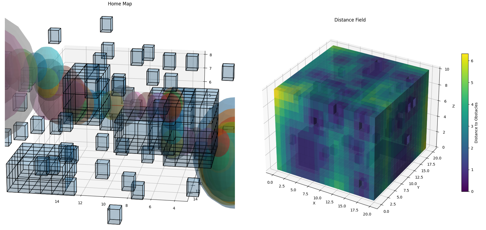
IV-A Surface Extraction Using Differential Geometry
IV-A1 Parametric Surface Representation
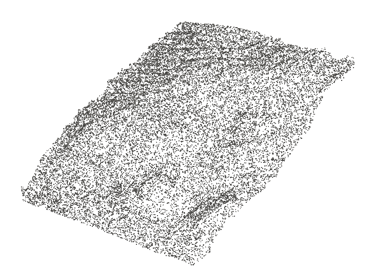
We represent the environment using a parametric surface based on the terrain point cloud collected from sensors:
| (1) |
where and are parameters defining the surface.
IV-A2 Differential Geometry Fundamentals
To capture the intrinsic properties of the surface, we compute the first and second fundamental forms.
First Fundamental Form:
| (2) |
where:
| (3) |
Second Fundamental Form:
| (4) |
where:
| (5) |
and is the unit normal vector:
| (6) |
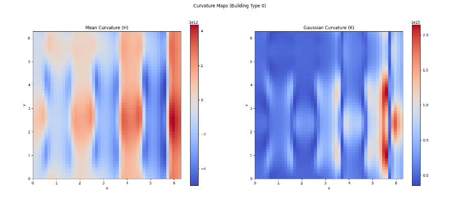
IV-A3 Curvature Computation
Gaussian Curvature :
| (7) |
Mean Curvature :
| (8) |
These curvature measures help in identifying critical regions on the surface for planning purposes.
IV-A4 Surface Smoothing and Protrusion Removal Using Curvature Analysis
To improve the accuracy of the elevation data and ensure the surface model is suitable for path planning, we utilize the Gaussian curvature and Mean curvature to identify and smooth out abrupt protrusions and irregularities on the surface.
Curvature-Based Filtering Algorithm
-
1.
Curvature Threshold Determination:
-
•
Calculate the statistical properties (mean and standard deviation ) of the Gaussian and Mean curvature values across the surface.
-
•
Set curvature thresholds:
(9) where and are scaling factors chosen based on the desired level of smoothing.
-
•
-
2.
Outlier Detection:
-
•
For each point on the surface, compute and .
-
•
Identify points where or as outliers or protrusions.
-
•
-
3.
Smoothing Procedure:
-
•
Apply a Laplacian smoothing algorithm to the identified outlier points:
(10) where is a smoothing factor, and is the Laplacian of , computed as the difference between the point and the average of its neighboring points.
-
•
-
4.
Iterative Refinement:
-
•
Repeat the outlier detection and smoothing steps until the maximum curvature values are below the set thresholds, ensuring a smooth surface.
-
•
-
5.
Preservation of Critical Features:
-
•
To avoid over-smoothing important terrain features, implement adaptive smoothing where varies based on local curvature values.
-
•
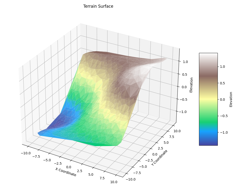
IV-A5 Elevation Coordinate Extraction
After obtaining a smooth surface, we proceed to extract the elevation coordinates essential for terrain analysis and path planning.
Elevation Extraction Algorithm
-
1.
Parameter Domain Discretization:
-
•
Define a grid over the parameter domain with appropriate resolution.
-
•
-
2.
Surface Point Evaluation:
-
•
Evaluate at each grid point to obtain the corresponding coordinates.
-
•
-
3.
Elevation Mapping:
-
•
Extract the -coordinate for each position to create an elevation map:
(11)
-
•
-
4.
Interpolation and Resampling:
-
•
Use interpolation methods (e.g., bilinear, bicubic) to fill in any gaps and create a continuous elevation surface.
-
•
-
5.
Post-processing:
-
•
Apply filters to remove any residual noise and enhance the terrain features, such as median or Gaussian filters.
-
•
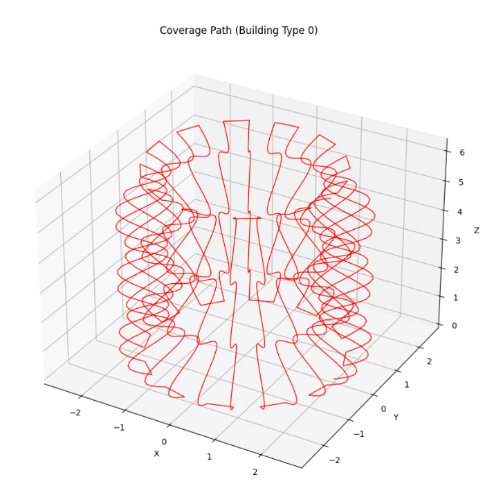
IV-B Direct Landmark Point Planning
To achieve efficient and complete coverage of the terrain, we propose a direct landmark point planning method that overlays a uniform grid of points onto the smoothed parametric surface. This approach eliminates the need for traditional cell decomposition and allows for a more straightforward implementation that adapts naturally to the terrain’s geometry.
IV-B1 Uniform Grid Generation on the Parametric Surface
We begin by discretizing the parameter domain of the smoothed surface to create a uniform grid of parameters . This grid serves as the foundation for the placement of landmark points on the terrain.
Parameter Domain Discretization:
Let and . We define:
| (12) |
where , , and , are the parameter increments.
IV-B2 Mapping Grid Points to 3D Surface Landmarks
Each grid point is mapped onto the 3D surface to obtain the corresponding landmark point .
Surface Point Evaluation:
| (13) |
Elevation Offset for Clearance:
To ensure the navigating agent maintains a safe distance above the terrain, an elevation offset is added:
| (14) |
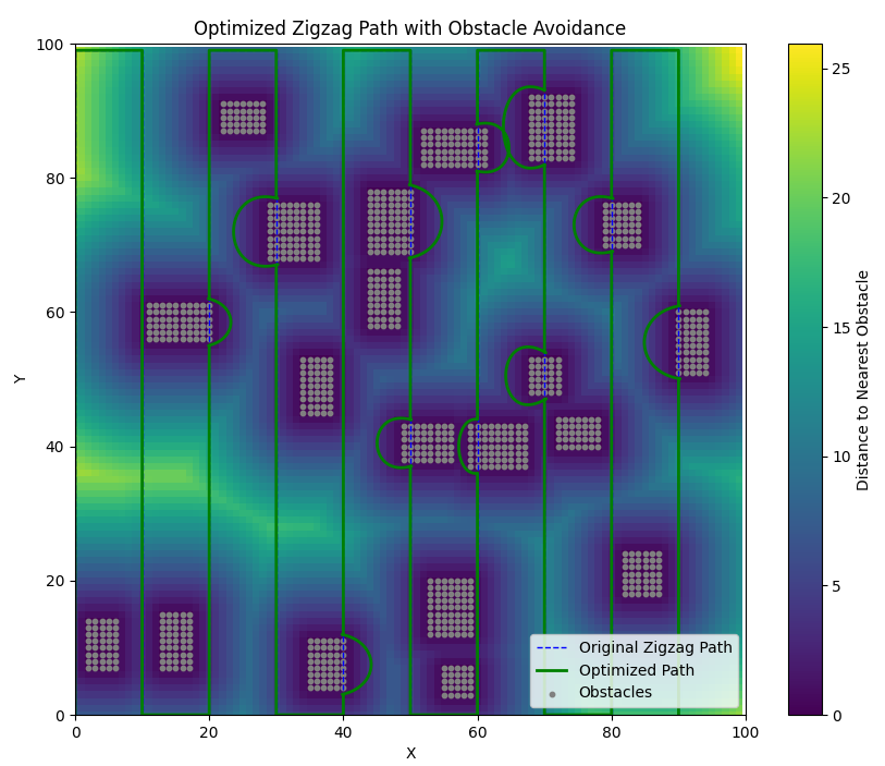
IV-B3 Coverage Path Planning Using a Boustrophedon Pattern
We sequence the adjusted landmark points in a boustrophedon (zigzag) pattern to ensure systematic and complete coverage of the terrain.
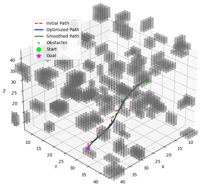
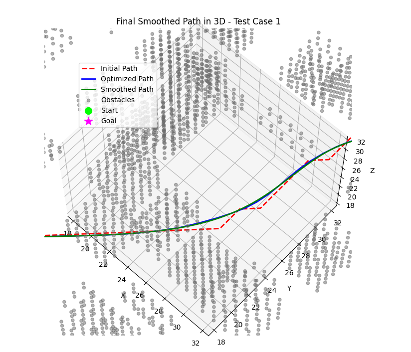
IV-C Dynamic Trajectory Planning with Safety Thresholds
To handle obstacles and narrow passages efficiently, we employ a two-stage path planning process.
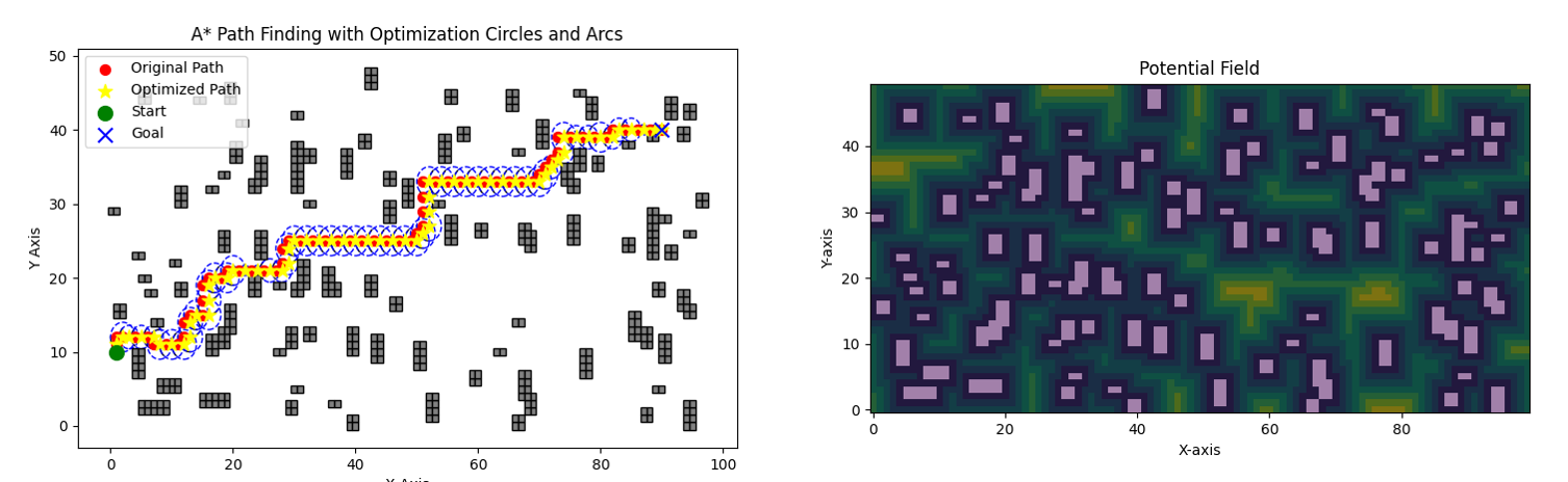
IV-C1 Global Path Planning
We use the A* algorithm with an enhanced heuristic that incorporates a potential field derived from obstacle distances.
Heuristic Function:
| (15) |
where:
-
•
: Cost from the start node to current node .
-
•
: Heuristic estimate from to the goal.
-
•
: Potential field function.
-
•
: Weighting factor.
IV-C2 Potential Field Calculation
We define the potential field based on the inverse of the distance to the nearest obstacle:
| (16) |
where is the Euclidean distance to the nearest obstacle, and is a small constant.
IV-C3 Local Optimization with Safety Thresholds
When a segment of the path is within a safety distance from obstacles, we perform local optimization.
Cost Function :
| (17) |
IV-D Dynamic Obstacle Avoidance and Path Optimization
In dynamic and complex environments, autonomous systems must adapt their planned trajectories in real-time to avoid obstacles while maintaining efficient coverage. We present an integrated approach that combines semantic mapping, path planning, and dynamic obstacle avoidance using monocular cameras and IMU-aligned data.
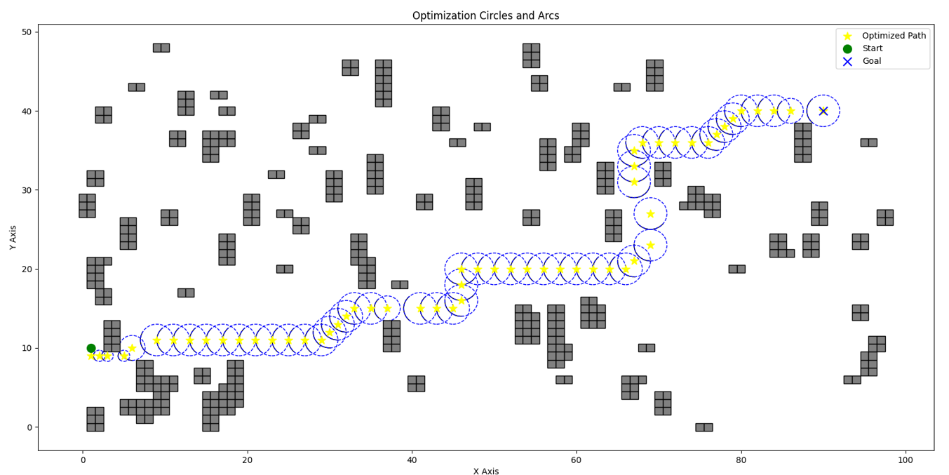
IV-D1 Circular Judgment and Assessment Module
IV-D2 Semantic Mapping and Localization
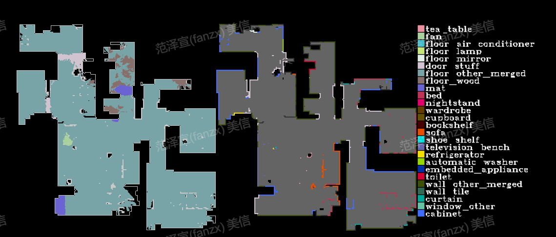
Our system generates a Panoptic Occupancy Local Semantic Map by processing data from monocular cameras and an IMU. This map provides detailed information about the environment, including the location and classification of obstacles. The localization information is aligned with the IMU data to accurately position the autonomous agent within the map.
IV-D3 Radiant Field-Informed Coverage Planning (RFICP)
To initiate the planning process, we utilize preloaded terrain data or previously established semantic information, such as a prior semantic map. We implement the proposed Radiant Field-Informed Coverage Planning (RFICP) algorithm, which computes coverage trajectories and velocity assignments for efficient path planning.
During navigation, the autonomous agent must continuously assess the planned path for compliance with safety and efficiency criteria, especially in the presence of dynamic obstacles. We introduce the Circular Judgment and Assessment Module to identify regions along the path that violate the defined path cost function due to obstacles or environmental changes.
Algorithm for Circular Judgment and Assessment
Algorithm 1: Circular Judgment and Assessment
Input: Current position , planned path , path cost function , threshold , detection radius .
Output: Set of non-compliant path segments .
-
1.
Initialize:
-
•
Set .
-
•
Define detection window centered at with radius .
-
•
-
2.
Identify Points within Window:
-
•
Extract path points such that .
-
•
-
3.
Evaluate Path Cost:
-
•
For each consecutive segment within :
-
–
Compute .
-
–
If :
-
*
Add to .
-
*
-
–
-
•
-
4.
Return .
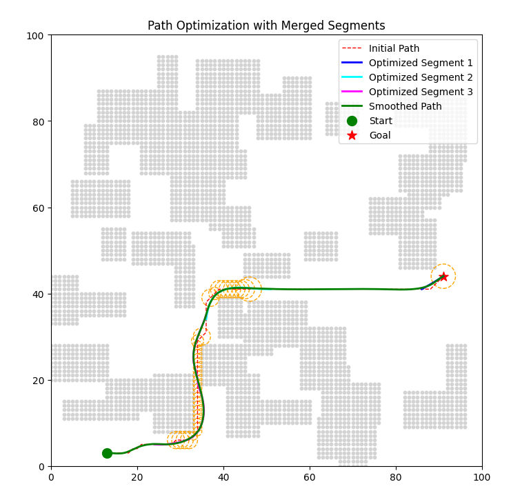
IV-D4 Incremental IKD-tree Sliding Window Optimization (IKD-SWOpt)
To optimize the identified non-compliant path segments , we introduce the Incremental IKD-tree Sliding Window Optimization (IKD-SWOpt) algorithm. This method leverages an incremental KD-tree for efficient obstacle representation and employs BFGS optimization to refine the path within a sliding window.
Algorithm 2: Incremental IKD-tree Sliding Window Optimization (IKD-SWOpt)
Input: Non-compliant path segments , obstacle data, initial path .
Output: Optimized path segments .
-
1.
Initialize:
-
•
Build incremental KD-tree from obstacle data.
-
•
Set initial variables as the concatenation of coordinates of .
-
•
-
2.
Define Cost Function:
(18) -
3.
Optimization Loop:
-
•
While not converged:
-
–
Compute gradient .
-
–
Update Hessian approximation .
-
–
Compute search direction .
-
–
Perform line search to find optimal step size .
-
–
Update variables:
(19)
-
–
-
•
-
4.
Update Path:
-
•
Extract optimized points from .
-
•
Replace in with optimized points.
-
•
-
5.
Return optimized path .
IV-E Trajectory Smoothing with B-Splines
To ensure smooth and continuous trajectories, we fit B-spline curves to the optimized waypoints.
IV-E1 B-Spline Curve Representation
| (20) |
where:
-
•
: Control points.
-
•
: B-spline basis functions of degree .
-
•
.
V Speed Planning Based on Environmental Attributes
V-A Coverage Model
V-A1 Circular Judgment and Assessment Module
The coverage effectiveness at a point depends on the robot’s speed and the time spent over that point.
Coverage Function: The cumulative coverage at point over time .
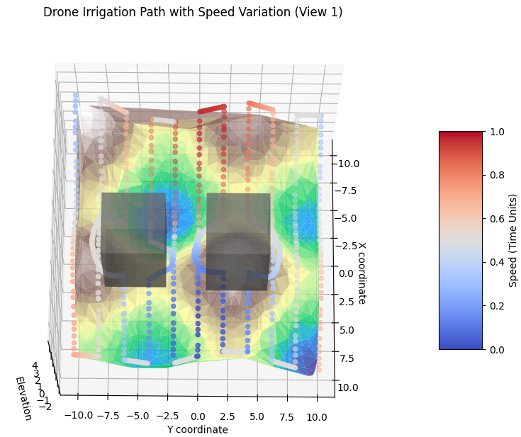
V-B Speed Adjustment Strategy in RFICP
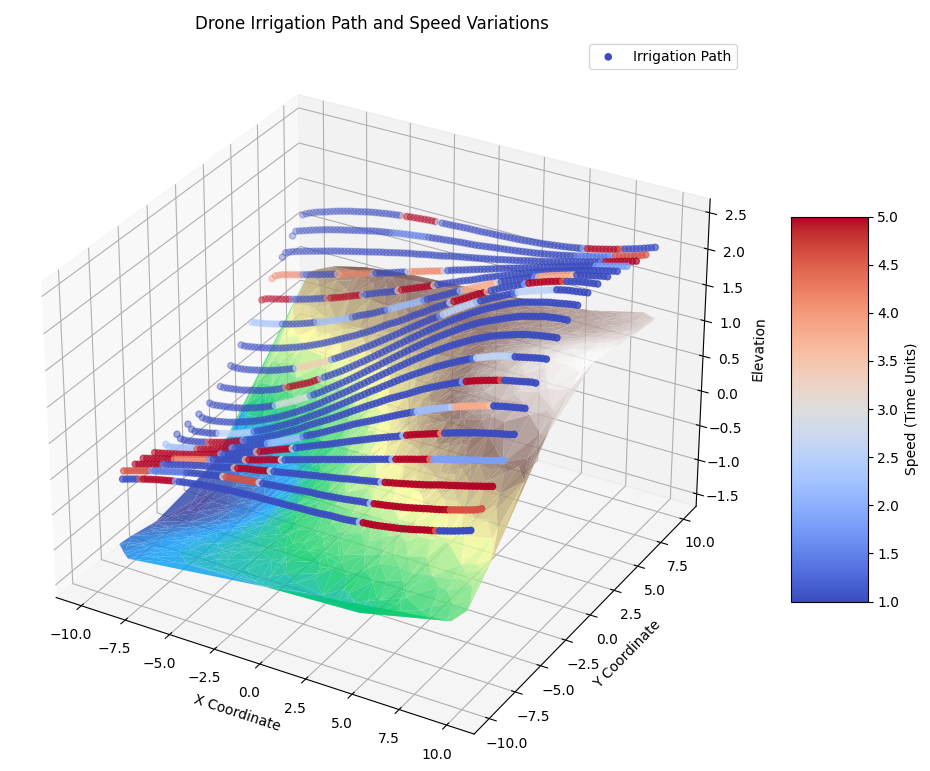
RFICP (Radiant Field-Informed Coverage Planning) leverages a diffusion field model to dynamically adjust the robot’s speed for uniform coverage across environments with varying attributes. By considering the radiant field effect, RFICP calculates optimal coverage time and speed to achieve desired efficiency while adhering to physical and operational constraints.
V-B1 Diffusion Field Model in RFICP
In RFICP, the diffusion field captures how a robot’s activity at one position influences surrounding areas. This model ensures that coverage is not treated in isolation but instead incorporates spatial relationships to achieve uniformity.
Gaussian Kernel Representation
The spatial influence of the robot’s activity is modeled using a Gaussian kernel:
| (21) |
V-B2 RFICP Desired Coverage Model
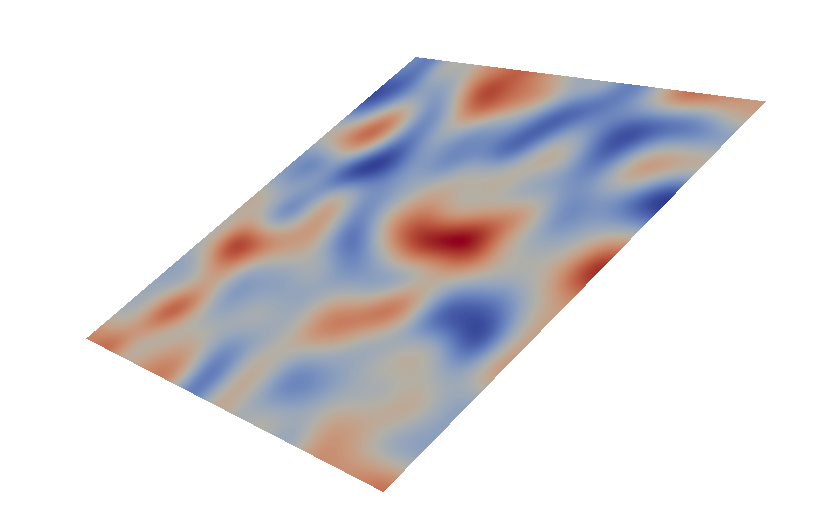
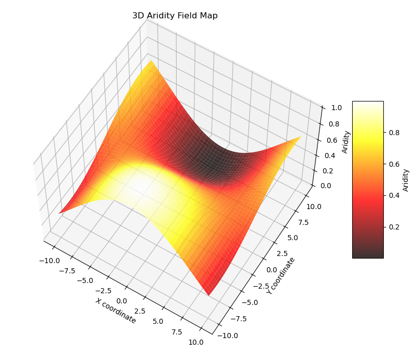
To address varying environmental attributes, RFICP sets a desired coverage proportional to the attribute , such as dirtiness or dryness:
| (22) |
V-B3 Time and Speed Planning in RFICP
Deriving Required Coverage Time
V-B4 Circular Judgment and Assessment Module
The time required to achieve the desired coverage can be derived by assuming the robot’s activity near dominates its effective coverage. Simplifying the total effective coverage:
| (23) |
Solving for :
| (24) |
Speed-Coverage Relationship
The robot’s speed is inversely related to the time :
| (25) |
V-B5 Implementation Framework of RFICP
The RFICP framework applies the speed adjustment strategy as follows:
-
1.
Initialization:
-
•
Input environmental attribute map , coverage parameters , and robot constraints .
-
•
-
2.
Coverage Time Computation:
-
•
Compute the required time at each position using the derived formula.
-
•
-
3.
Dynamic Speed Planning:
-
•
Derive speed from .
-
•
Smooth speed transitions by enforcing acceleration limits.
-
•
-
4.
Trajectory Integration:
-
•
Integrate the computed speed profile into the global trajectory, ensuring smooth and efficient coverage.
-
•
VI Experiments
VI-A Experimental Setup
VI-A1 Real-World Environment
Platforms:
-
•
Robotic Vacuum Cleaner: Tested in indoor environments with varying levels of dirtiness.

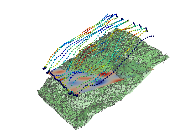
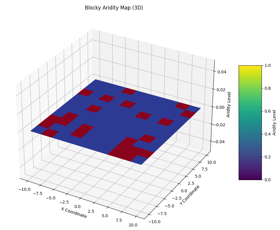
Figure 12: Real robot coverage in a semantic-labeled dirty environment: The robot adjusts its speed and coverage density according to detected dirtiness levels (blue-to-red colormap), integrating seamlessly with the SHIFT Planner’s adaptive strategies. Fig. 12 shows a real robot scenario in a semantic-labeled environment (dirtiness map). The robot, guided by SHIFT, slows down in dirty areas to ensure thorough coverage, and speeds up in cleaner regions to optimize efficiency.
VI-B Additional Comparative Experiments
-
•
Agricultural Drone: Tested in outdoor terrains with varying crop conditions.
Sensors: LiDAR, camera, IMU, odometer.
VI-B1 Data Collection
-
•
Terrain Point Clouds: Collected using onboard LiDAR sensors.
-
•
Environmental Attributes: Dirtiness levels detected using camera sensors and semantic segmentation.
VI-C Results and Analysis
VI-C1 Path Planning Efficiency
Our method efficiently generates feasible paths without the need for complex region decomposition.
VI-C2 Circular Judgment and Assessment Module
-
•
Computation Time: Reduced by approximately 30% compared to traditional methods.
-
•
Memory Usage: Lower due to the elimination of cell decomposition data structures.
VI-C3 Optimization Performance
The local optimization effectively adjusts the trajectory in critical areas.
-
•
Convergence: The optimization converges within a few iterations due to the analytical gradient computation.
-
•
Safety Margin: Maintained a safe distance from obstacles, improving overall safety.
VI-D Comparative Analysis with Existing Methods
To validate the performance of the proposed framework, we conducted a comparative analysis against state-of-the-art methods commonly used in coverage path planning. Table I summarizes the performance results.
Comparative Evaluation Metrics
-
1.
Coverage Completeness (%): The percentage of the area covered within the specified time limit.
-
2.
Computational Cost (s): Time taken to generate a coverage path.
-
3.
Path Overlap Rate (%): The percentage of the path that overlaps with previously covered areas.
-
4.
Energy Efficiency (Normalized Units): A normalized measure of energy consumption.
In this paper, we have presented a novel uniform coverage planning and navigation framework for autonomous robots operating in complex and dynamic environments. Leveraging data from monocular cameras and IMU alignment, we generate Panoptic Occupancy local semantic maps and accurate localization information. This is integrated with either preloaded terrain data or previously established semantic information to initialize the planning process.
We introduce the Radiant Field-Informed Coverage Planning (RFICP) algorithm, which incorporates a diffusion field model to dynamically adjust the robot’s speed and trajectory based on environmental attributes. By modeling the spatial influence of the robot’s actions using a Gaussian kernel, RFICP enables efficient and uniform coverage in areas with varying attributes (e.g., dirtiness, dryness). This approach allows the robot to adapt its behavior to local conditions, improving coverage uniformity and task effectiveness while adhering to physical and operational constraints.
When dynamic obstacles are encountered along the planned path, we propose a rapid path optimization method called Incremental IKD-tree Sliding Window Optimization (IKD-SWOpt) for obstacle avoidance. IKD-SWOpt continuously monitors the path within a sliding circular detection window—referred to as the Circular Judgment and Assessment Module—to identify regions that violate the defined path cost function. These segments are incorporated into an Adaptive Sliding Window for localized optimization, iteratively refining the trajectory until a collision-free path is achieved. This method enhances the robot’s ability to navigate safely in dynamic environments by providing efficient and responsive path adjustments.
The final phase of the framework focuses on trajectory tracking, ensuring accurate execution of the planned and optimized path. By integrating semantic mapping, coverage planning, dynamic obstacle avoidance, and trajectory tracking, our method enhances efficiency and adaptability in complex environments.
Acknowledgments
References
- [1] E. Galceran and M. Carreras, “A survey on coverage path planning for robotics,” Robotics and Autonomous Systems, vol. 61, no. 12, pp. 1258–1276, 2013.
- [2] H. Choset and J. Burdick, “Sensor-based exploration: The hierarchical generalized Voronoi graph,” The International Journal of Robotics Research, vol. 19, no. 2, pp. 96–125, 2000.
- [3] H. Choset and P. Pignon, “Coverage path planning: The boustrophedon cellular decomposition,” in Field and Service Robotics, pp. 203–209, Springer, 1997.
- [4] S. M. LaValle, “Rapidly-exploring random trees: A new tool for path planning,” Technical Report TR 98-11, Iowa State University, 1998.
- [5] C. Cao, J. Zhang, M. Travers, and H. Choset, “Hierarchical coverage path planning in complex 3D environments,” in Proceedings of the IEEE International Conference on Robotics and Automation (ICRA), 2020.
- [6] W. Jing, J. Polden, W. Lin, and K. Shimada, “Sampling-based view planning for 3D visual coverage task with unmanned aerial vehicle,” in Proceedings of the IEEE/RSJ International Conference on Intelligent Robots and Systems (IROS), 2016.
- [7] C. Feng, H. Li, M. Zhang, X. Chen, B. Zhou, and S. Shen, “FC-Planner: A skeleton-guided planning framework for fast aerial coverage of complex 3D scenes,” 2023.
- [8] A. Smith and B. Lee, “Collaborative complete coverage path planning,” International Journal of Robotics Research, vol. 39, no. 5, pp. 567–580, 2020.
- [9] K. Johnson and R. Patel, “K-Means clustering with deep reinforcement learning for coverage path planning,” IEEE Transactions on Automation Science and Engineering, vol. 16, no. 4, pp. 1525–1536, 2019.