Shape-aware Graph Spectral Learning

Several studies (Bo et al., 2021; Zhu et al., 2020a) have empirically shown that low-frequency information plays a crucial role in homophilous graphs, while high-frequency information is more important for heterophilous graphs. However, none of them provide theoretical evidence to support this observation. To fill this gap, we theoretically analyze the relationship between homophily ratio and graph frequency. Specifically, we examine two graph filters that exhibit distinct behaviors in different frequency regions and explore their impacts on graphs with varying homophily ratios.

The proof is in Appendix A.1. Lemma 3.1 reveals that if the edge set is constructed by random sampling, the expected homophily ratio of the graph is $1/C$. Hence, for a graph $\mathcal{G}$, if $h(\mathcal{G})>1/C$, it is more prone to generate homophilous edges than in the random case. If $h(\mathcal{G})<1/C$, heterophilous edges are more likely to form.

Note that in the theorem, we assume $g_{1}$ and $g_{2}$ have the same norm to avoid trivial solutions. The proof of the theorem and the discussion of this assumption is in Appendix A.2. Theorem 3.2 reveals that if $g_{1}$ has higher amplitude in the high-frequency region and lower amplitude in the low-frequency region compared to $g_{2}$, it will result in less similarity in representations of connected nodes. In contrast, $g_{2}$ increases the representation similarity of connected nodes. As most edges in heterophilous graphs are heterophilous edges, $g_{1}$ is preferred to increase distances between heterophilously connected nodes. In contrast, homophilous graphs prefer $g_{2}$ to decrease distances between homophilously connected nodes. Next, we theoretically prove the claim that low-frequency is beneficial for the prediction of homophilous graphs, while high-frequency is beneficial for heterophilous graphs.

The proof is in Appendix A.3. In Theorem 3.3, $\Delta\bar{d}$ shows the discriminative ability of the learned representation, where a large $\Delta\bar{d}$ indicates that representations of intra-class nodes are similar, while representations of inter-class nodes are dissimilar. As $g_{1}$ and $g_{2}$ are defined as described in Theorem 3.2, we can guarantee $\mathbb{E}[\Delta s]>0$. Hence, homophilous graphs with $h>1/C$ favor $g_{1}$; while heterophilous graphs with $h<1/C$ favor $g_{2}$. This theorem shows that the transition phase of a balanced graph is $1/C$, where the transition phase is the point whether lower or higher frequencies are more beneficial changes.

Theorem 3.2 and Theorem 3.3 together guide us to the desired filter shape. When $h>1/C$, the filter should involve more low-frequency and less high-frequency. When $h<1/C$, the filter need to decrease the low-frequency and increase the high-frequency to be more discriminative.

With the theoretical understanding, in this subsection, we further empirically analyze and verify the influence of high- and low- frequencies on node classification performance on graphs with various homophily ratios, which help us to design better GNN for node classification. As high-frequency and low-frequency are relative concepts, there is no clear division between them. Therefore, to make the granularity of our experiments better and to make our candidate filters more flexible, we divide the graph spectrum into three parts: low-frequency $0\leq\lambda_{low}<\frac{2}{3}$, middle-frequency $\frac{2}{3}\leq\lambda_{mid}<\frac{4}{3}$, and high-frequency $\frac{4}{3}\leq\lambda_{high}\leq 2$. We perform experiments on synthetic datasets generated by contextual stochastic block model (CSBM) (Deshpande et al., 2018), which is a popular model that allows us to create synthetic attributed graphs with controllable homophily ratios (Ma et al., 2022; Chien et al., 2021). A detailed description of CSBM is in Appendix D.1.

To analyze which parts of frequencies in the graph spectrum are beneficial or harmful for graphs with different homophily ratios, we conduct the following experiments. We first generate synthetic graphs with different homophily ratios as $\{0,0.05,0.10,\cdots,1.0\}$. Then for each graph, we conduct eigendecomposition as $\mathbf{L}=\mathbf{U}\mathbf{\Lambda}\mathbf{U}^{\top}$ and divide the eigenvalues into three parts: low-frequency $0\leq\lambda_{low}<\frac{2}{3}$, middle-frequency $\frac{2}{3}\leq\lambda_{mid}<\frac{4}{3}$, and high-frequency $\frac{4}{3}\leq\lambda_{high}\leq 2$, because three-part provides more flexibility of the filter. As shown in Fig. LABEL:fig:mag_imp(a), we vary the output values of the filter, i.e., amplitudes of $g(\lambda_{low}),g(\lambda_{mid})$, and $g(\lambda_{high})$ among $\{0,0.4,0.8,1.2,1.6,2.0\}$ respectively, which leads to $6^{3}$ combinations of output values of the filter. Then we get transformed graph Laplacian $g(\mathbf{L})=\mathbf{U}g(\mathbf{\Lambda})\mathbf{U}^{\top}$. For each filter, we use $g(\mathbf{L})$ as a convolutional matrix to learn node representation as $\mathbf{Z}=g(\mathbf{L})f_{\theta}(\mathbf{X})$, where $f_{\theta}$ is the feature transformation function implemented by an MLP. In summary, the final node representation is given by $\mathbf{z}=\mathbf{U}\operatorname{diag}\left[g(\lambda_{low}),g(\lambda_{mid}),g(\lambda_{high})\right]\mathbf{U}^{\top}f_{\theta}(\mathbf{x})$. By varying the amplitudes of each part of frequency, we vary how much a certain frequency is included in the representations. For example, the larger the value of $g(\lambda_{low})$ is, the more low-frequency information is included in $\mathbf{z}$. We then add a Softmax layer on top of $\mathbf{Z}$ to predict the label of each node. For each synthetic graph, we split the nodes into 2.5%/2.5%/95% for train/validation/test. For each filter, we conduct semi-supervised node classification on each synthetic graph and record the classification performance.

Frequency Importance. With the above experiments, to understand which filter works best for which homophily ratio, for each homophily ratio, we first select filters that give top 5% performance among the $6^{3}$ filters. Let $\mathcal{F}_{h}=\{[g_{h}^{i}(\lambda_{low}),g_{h}^{i}(\lambda_{mid}),g_{h}^{i}(\lambda_{high})]\}_{i=1}^{K}$ be the set of the best filters for homophily ratio $h$, where $[g_{h}^{i}(\lambda_{low}),g_{h}^{i}(\lambda_{mid}),g_{h}^{i}(\lambda_{high})]$ means the $i$-th best filter for $h$ and $K$ is the number of best filters. Then, importance scores of low, middle, and high frequency are given as

$$\small\begin{split}\mathcal{I}_{h}^{low}&=\frac{1}{|\mathcal{F}_{h}|}{\sum}_{i=1}^{|\mathcal{F}_{h}|}g_{h}^{i}(\lambda_{low}),\quad\mathcal{I}_{h}^{mid}=\frac{1}{|\mathcal{F}_{h}|}{\sum}_{i=1}^{|\mathcal{F}_{h}|}g_{h}^{i}(\lambda_{mid}),\\ \mathcal{I}_{h}^{high}&=\frac{1}{|\mathcal{F}_{h}|}{\sum}_{i=1}^{|\mathcal{F}_{h}|}g_{h}^{i}(\lambda_{high}).\end{split}$$

(3)

The importance score of a certain frequency shows how much that frequency should be involved in the representation to achieve the best performance. The findings in Fig. LABEL:fig:mag_imp(b) reveal two important observations: (i) as the homophily ratio increases, there is a notable increase in the importance of low-frequency, a peak and subsequent decline in the importance of middle-frequency, and a decrease in the importance of high-frequency; (ii) the transition phase occurs around the homophily ratio of $1/2$ as there are two distinct classes, resulting in a significant shift in the importance of frequencies. The frequency importance of graphs generated with other parameters is in Appendix E.3. These observations guide us in designing the spectral filter. For high-homophily graphs, we want to preserve more low-frequency while removing high frequencies. For low-homophily graphs, more high frequencies and fewer low frequencies are desired. For graphs with homophily ratios near the transition phase, we aim the model to learn adaptively.

In order to learn flexible filters and incorporate prior knowledge in Section 3 in the filter, i.e., encouraging or discouraging different frequencies based on the homophily ratio, we first propose to adopt a set of $K+1$ learnable points $\mathcal{S}=\{(q_{0},t_{0}),\cdots,(q_{n},t_{K})\}$ of the filter. Interpolated points $\mathbf{q}=[q_{0},\cdots,q_{K}]$ are fixed and distributed equally among low, middle, and high-frequency depending on their values. The corresponding values $\mathbf{t}=[t_{0},\cdots,t_{K}]$ are learnable and updated in each epoch of training. These learnable points gives the basic shape of a filter. Then we can use interpolation method to approximate a filter function $g$ by passing these points such that $g(q_{k})=t_{k}$, where $0\leq k\leq K$. This gives us two advantages: (i) As $\mathbf{t}$ determines the basic shape of a filter $g$ and is learnable, we can learn arbitrary filter by learning $\mathbf{t}$ that minimizes the node classification loss; and (ii) As the filter $g$ is determined by $\mathbf{t}$, it allows us to add regularization on $\mathbf{t}$ to encourage beneficial and discourage harmful frequencies based on homophily ratio.

Specifically, with these points, we adopt Newton Interpolation (Hildebrand, 1987) to learn the filter, which is a widely-used method for approximating a function by fitting a polynomial on a set of given points. Given $K+1$ points and their values $\mathcal{S}=\{(q_{0},t_{0}),\cdots,(q_{n},t_{K})\}$ of an unknown function $g$, where $q_{k}$ are pairwise distinct, $g$ can be interpolated based on Newton Interpolation as follows.

Eq. 5 satisfies $g(q_{k})=t_{k}$ and $K$ is the power of the polynomial. As mentioned in Eq. 2, we directly apply the spectral filter $g$ on Laplacian $\mathbf{L}$ to get the final representations. Then Eq. 5 is reformulated as $g(\mathbf{L})={\sum}_{k=0}^{K}\left\{\hat{g}_{\mathbf{t}}[q_{0},\cdots,q_{k}]{\prod}_{i=0}^{k-1}(\mathbf{L}-q_{i}\mathbf{I})\right\}$, where $\mathbf{I}$ is the identity matrix.

Following (Chien et al., 2021), to increase the expressive power, the node features are firstly transformed by a transformation layer $f_{\theta}$, then a convolutional matrix learned by NewtonNet is applied to transformed features, which is shown in Fig. 2. Mathematically, NewtonNet can be formulated as:

$$\mathbf{Z}={\sum}_{k=0}^{K}\left\{\hat{g}_{\mathbf{t}}[q_{0},\cdots,q_{k}]{\prod}_{i=0}^{k-1}(\mathbf{L}-q_{i}\mathbf{I})\right\}f_{\theta}(\mathbf{X}),$$

(6)

where $f_{\theta}$ is a feature transformation function, and we use a two-layer MLP in this paper. $q_{0},\cdots,q_{K}$ can be any points $\in[0,2]$. We use the equal-spaced points, i.e., $q_{i}=2i/K$. $q_{i}$ controls different frequencies depending on its value. $t_{0},\cdots,t_{K}$ are learnable filter output values and are randomly initialized. By learning $t_{i}$, we are not only able to learn arbitrary filters, but can also apply regularization on $t_{i}$’s to adapt the filter based on homophily ratio, which will be discussed in Section 4.2. With the node representation $\mathbf{z}_{v}$ of node $v$, $v$’s label distribution probability is predicted as $\hat{\boldsymbol{y}}_{v}=\operatorname{softmax}(\mathbf{z}_{v})$.

As $\{t_{0},\cdots,t_{k}\}$ determines the shape of filter $g$, we can control the filter shape by adding constraints on learned function values. As shown in Fig. 2, we slice $\mathbf{t}$ into three parts

$$\begin{split}\mathbf{t}_{low}&=[t_{0},\cdots,t_{i-1}],\ \mathbf{t}_{mid}=[t_{i},\cdots,t_{j-1}],\\ \mathbf{t}_{high}&=[t_{j},\cdots,t_{K}],\quad 0<i<j<K,\end{split}$$

(7)

which represent the amplitude of low, middle, and high-frequency, respectively. In this paper, we set $K=5,i=2,j=4$ so that we have six learnable points and two for each frequency. According to the analysis results in Section 3, as the homophily ratio increases, we design the following regularizations. (i) For low-frequency, the amplitude should decrease, and we discourage low-frequency before the transition phase and encourage it after the transition phase. Thus, we add a loss term as $\left(\frac{1}{C}-h\right)\|\mathbf{t}_{low}\|_{2}^{2}$ to regularize the amplitudes of low-frequency. When the homophily ratio is smaller than the transition phase $1/C$, the low-frequency is harmful; therefore, the loss term has a positive coefficient. In contrast, when the homophily ratio is larger than the transition phase, the low-frequency is beneficial, and we give a positive coefficient for the loss term. (ii) For high-frequency, the amplitude should decrease, and we encourage the high-frequency before the transition phase and discourage it after the transition phase. Similarly, the regularization for high-frequency is $\left(h-\frac{1}{C}\right)\|\mathbf{t}_{high}\|_{2}^{2}$. (iii) For middle-frequency, we observe that it has the same trend as the low-frequency before the transition phase and has the same trend as the high-frequency after the transition phase in Fig. LABEL:fig:mag_imp (b). Therefore, we have the regularization $\left|h-\frac{1}{C}\right|\|\mathbf{t}_{mid}\|_{2}^{2}$. These three regularization work together to determine the shape based on homophily ratio $h$. Then the shape-aware regularization can be expressed as

$$\begin{split}\min_{\theta,\mathbf{t}}\mathcal{L}_{SR}&=\gamma_{1}\left(\frac{1}{C}-h\right)\|\mathbf{t}_{low}\|_{2}^{2}+\\ &\gamma_{2}\left|h-\frac{1}{C}\right|\|\mathbf{t}_{mid}\|_{2}^{2}+\gamma_{3}\left(h-\frac{1}{C}\right)\|\mathbf{t}_{high}\|_{2}^{2},\end{split}$$

(8)

where $\gamma_{1},\gamma_{2},\gamma_{3}>0$ are scalars to control contribution of the regularizers, respectively. $h$ is the learned homophily ratio, calculated and updated according to the labels learned in every epoch. The final objective function of NewtonNet is

$$\min_{\theta,\mathbf{t}}\mathcal{L}=\mathcal{L}_{CE}+\mathcal{L}_{SR},$$

(9)

where $\mathcal{L}_{CE}={\sum}_{v\in\mathcal{V}^{L}}\ell(\hat{\boldsymbol{y}}_{v},\boldsymbol{y}_{v})$ is classification loss on labeled nodes and $\ell(\cdot,\cdot)$ denotes cross entropy loss. The training algorithm of NewtonNet is in Appendix B.

Compared with other approximation and interpolation methods This Newton Interpolation method has its advantages compared with approximation methods, e.g., ChebNet (Defferrard et al., 2016), GPRGNN (Chien et al., 2021), and BernNet (He et al., 2021b). Both interpolation and approximation are common methods to approximate a polynomial function. However, the interpolation function passes all the given points accurately, while approximation methods minimize the error between the function and given points. We further discuss the difference between interpolation and approximation methods in Appendix C. This difference makes us be able to readily apply shape-aware regularization on learned $\mathbf{t}$. However, approximation methods do not pass given points accurately, so we cannot make points learnable to approximate arbitrary functions and apply regularization.

Compared to other interpolation methods like ChebNetII (He et al., 2022), Newton interpolation offers greater flexibility in choosing interpolated points. In Eq. 6, $q_{i}$ values can be freely selected from the range [0, 2], allowing adaptation to specific graph properties. In contrast, ChebNetII uses fixed Chebyshev points for input values, limiting precision in narrow regions and requiring increased complexity (larger K) to address this limitation. Additionally, ChebNetII can be seen as a special case of NewtonNet when Chebyshev points are used as $q_{i}$ values (He et al., 2022).

Complexity Analysis NewtonNet exhibits a time complexity of $O(KEF+NF^{2})$ and a space complexity of $O(KE+F^{2}+NF)$, where $E$ represents the number of edges. Notably, the complexity scales linearly with $K$. A detailed analysis is provided in Appendix B.1.

We use node classification to evaluate the performance. Here we briefly introduce the dataset, baselines, and settings in the experiments. We give details in Appendix D.

Baselines. We compare NewtonNet with representative baselines, including (i) non-topology method: MLP; (ii) spatial methods: GCN (Kipf & Welling, 2017), Mixhop (Abu-El-Haija et al., 2019), APPNP (Klicpera et al., 2018), GloGNN++ (Li et al., 2022); and (iii) spectral methods: ChebNet (Defferrard et al., 2016), GPRGNN (Chien et al., 2021), BernNet (He et al., 2021b), ChebNetII (He et al., 2022), JacobiConv (Wang & Zhang, 2022). Details of methods are in Appendix D.3.

Settings. We adopt the commonly-used split of 60%/20%/20% for train/validation/test sets. For a fair comparison, for each method, we select the best configuration of hyperparameters using the validation set and report the mean accuracy and variance of 10 random splits on the test.

Table 1 shows the results on node classification, where boldface denotes the best results and underline denotes the second-best results. We observe that learnable spectral GNNs outperform other baselines since spectral methods can learn beneficial frequencies for prediction under supervision, while spatial methods and predetermined spectral methods only obtain information from certain frequencies. NewtonNet achieves state-of-the-art performance on eight of nine datasets with both homophily and heterophily, and it achieves the second-best result on Cora. This is because NewtonNet efficiently learns the filter shape through Newton interpolation and shape-aware regularization.

As we mentioned before, learning filters solely based on the downstream tasks may lead to suboptimal performance, especially when there are rare labels. Thus, this subsection delves into the impact of the training ratio on the performance of various GNNs. We keep the validation and test set ratios fixed at 20%, and vary the training set ratio from $0.1$ to $0.6$. We select several best-performing baselines and plot their performance on the Chameleon and Squirrel datasets in Fig. LABEL:fig:vary_ratio. From the figure, we observe: (1) When the training ratio is large, spectral methods perform well because they have sufficient labels to learn a filter shape. Conversely, when the training ratio is small, some spectral methods do not perform as well as GCN as there are not enough labels for the models to learn the filter; (2) NewtonNet consistently outperforms all baselines. When the training ratio is large, NewtonNet can filter out harmful frequencies while encouraging beneficial ones, leading to representations of higher quality. When the training ratio is small, the shape-aware regularization of NewtonNet incorporates prior knowledge to provide guidance in learning better filters.

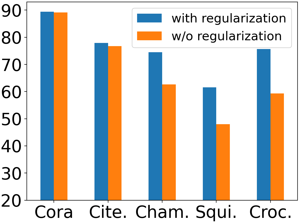
Next, we study the effect of shape-aware regularization on node classification performance. We show the best result of NewtonNet with and without shape-aware regularization, where we use the same search space as in Section 6.2. Fig. 4 gives the results on five datasets. From the figure, we can observe that the regularization contributes more to the performance on heterophilous datasets (Chameleon, Squirrel, Crocodile) than on homophilous datasets (Cora, Citeseer). The reason is as follows. Theorem 3.3 and Fig. LABEL:fig:mag_imp(b) show that the importance of frequencies changes significantly near the transition phase, $1/C$. Cora and Citeseer have homophily ratios of 0.81 and 0.74, while they have 7 and 6 classes, respectively. Since Cora and Citeseer are highly homophilous datasets whose homophily ratios are far from the transition faces, almost only low frequencies are beneficial, and thus the filter shapes are easier to learn. By contrast, the homophily ratios of Chameleon, Squirrel, and Crocodile are 0.24, 0.22, and 0.25, respectively, while they have five classes. Their homophily ratios are around the transition phase; therefore, the model relies more on shape-aware regularization to guide the learning process. We also conduct the hyperparameter analysis for $\gamma_{1}$, $\gamma_{2}$, $\gamma_{3}$, and $K$ in Appendix E.1.

Here we present the learned filters of NewtonNet on Citeseer and Chameleon and compare them with those learned by BernNet and ChebNetII. In Fig. LABEL:fig:learned_on_citeseer_chameleon, we plot the average filters by calculating the average temperatures of 10 splits. On the homophilous graph Citeseer, NewtonNet encourages low-frequency and filters out middle and high-frequency, which is beneficial for the representations of homophilous graphs. In contrast, ChebNetII and BernNet do not incorporate any shape-aware regularization, and their learning processes include middle and high-frequency, harming the representations of homophilous graphs. On the heterophilous dataset Penn94, the filter learned by NewtonNet contains more high-frequency and less-frequency, while harmful frequencies are included in the filters learned by ChebNetII and BernNet. These results reveal that NewtonNet, with its shape-aware regularization, can learn a filter shape with beneficial frequencies while filtering out harmful frequencies. More results of the learned filters can be found in Appendix E.4. We also present the learned homophily ratio in Appendix E.2.

References

- Abu-El-Haija et al. (2019) Abu-El-Haija, S., Perozzi, B., Kapoor, A., Alipourfard, N., Lerman, K., Harutyunyan, H., Ver Steeg, G., and Galstyan, A. Mixhop: Higher-order graph convolutional architectures via sparsified neighborhood mixing. In ICML, pp. 21–29. PMLR, 2019.
- Blakely et al. (2021) Blakely, D., Lanchantin, J., and Qi, Y. Time and space complexity of graph convolutional networks. Accessed on: Dec, 31, 2021.
- Bo et al. (2021) Bo, D., Wang, X., Shi, C., and Shen, H. Beyond low-frequency information in graph convolutional networks. In Proceedings of the AAAI Conference on Artificial Intelligence, volume 35, pp. 3950–3957, 2021.
- Bo et al. (2023) Bo, D., Wang, X., Liu, Y., Fang, Y., Li, Y., and Shi, C. A survey on spectral graph neural networks. arXiv preprint arXiv:2302.05631, 2023.
- Chien et al. (2021) Chien, E., Peng, J., Li, P., and Milenkovic, O. Adaptive universal generalized pagerank graph neural network. In ICLR, 2021.
- Dai et al. (2022) Dai, E., Zhou, S., Guo, Z., and Wang, S. Label-wise graph convolutional network for heterophilic graphs. In Learning on Graphs Conference, 2022.
- Defferrard et al. (2016) Defferrard, M., Bresson, X., and Vandergheynst, P. Convolutional neural networks on graphs with fast localized spectral filtering. NeurIPS, 29, 2016.
- Deshpande et al. (2018) Deshpande, Y., Sen, S., Montanari, A., and Mossel, E. Contextual stochastic block models. Advances in Neural Information Processing Systems, 31, 2018.
- Fout et al. (2017) Fout, A., Byrd, J., Shariat, B., and Ben-Hur, A. Protein interface prediction using graph convolutional networks. Advances in neural information processing systems, 30, 2017.
- Gilmer et al. (2017) Gilmer, J., Schoenholz, S. S., Riley, P. F., Vinyals, O., and Dahl, G. E. Neural message passing for quantum chemistry. In International conference on machine learning, pp. 1263–1272. PMLR, 2017.
- Hamilton et al. (2017) Hamilton, W., Ying, Z., and Leskovec, J. Inductive representation learning on large graphs. Advances in neural information processing systems, 30, 2017.
- He et al. (2021a) He, D., Liang, C., Liu, H., Wen, M., Jiao, P., and Feng, Z. Block modeling-guided graph convolutional neural networks. arXiv preprint arXiv:2112.13507, 2021a.
- He et al. (2021b) He, M., Wei, Z., Xu, H., et al. Bernnet: Learning arbitrary graph spectral filters via bernstein approximation. Advances in Neural Information Processing Systems, 34:14239–14251, 2021b.
- He et al. (2022) He, M., Wei, Z., and Wen, J.-R. Convolutional neural networks on graphs with chebyshev approximation, revisited. In NeurIPS, 2022.
- Hildebrand (1987) Hildebrand, F. B. Introduction to numerical analysis. Courier Corporation, 1987.
- Kipf & Welling (2016) Kipf, T. N. and Welling, M. Variational graph auto-encoders. arXiv preprint arXiv:1611.07308, 2016.
- Kipf & Welling (2017) Kipf, T. N. and Welling, M. Semi-supervised classification with graph convolutional networks. In ICLR, 2017.
- Klicpera et al. (2018) Klicpera, J., Bojchevski, A., and Günnemann, S. Predict then propagate: Graph neural networks meet personalized pagerank. arXiv preprint arXiv:1810.05997, 2018.
- Levie et al. (2018) Levie, R., Monti, F., Bresson, X., and Bronstein, M. M. Cayleynets: Graph convolutional neural networks with complex rational spectral filters. IEEE Transactions on Signal Processing, 67(1):97–109, 2018.
- Li et al. (2021) Li, S., Kim, D., and Wang, Q. Beyond low-pass filters: Adaptive feature propagation on graphs. In Machine Learning and Knowledge Discovery in Databases. Research Track: European Conference, ECML PKDD 2021, Bilbao, Spain, September 13–17, 2021, Proceedings, Part II 21, pp. 450–465. Springer, 2021.
- Li et al. (2022) Li, X., Zhu, R., Cheng, Y., Shan, C., Luo, S., Li, D., and Qian, W. Finding global homophily in graph neural networks when meeting heterophily. In International Conference on Machine Learning, pp. 13242–13256. PMLR, 2022.
- Lim & Benson (2021) Lim, D. and Benson, A. R. Expertise and dynamics within crowdsourced musical knowledge curation: A case study of the genius platform. In Proceedings of the International AAAI Conference on Web and Social Media, volume 15, pp. 373–384, 2021.
- Lim et al. (2021) Lim, D., Hohne, F., Li, X., Huang, S. L., Gupta, V., Bhalerao, O., and Lim, S. N. Large scale learning on non-homophilous graphs: New benchmarks and strong simple methods. Advances in Neural Information Processing Systems, 34:20887–20902, 2021.
- Liu et al. (2022) Liu, N., Wang, X., Bo, D., Shi, C., and Pei, J. Revisiting graph contrastive learning from the perspective of graph spectrum. In Oh, A. H., Agarwal, A., Belgrave, D., and Cho, K. (eds.), Advances in Neural Information Processing Systems, 2022. URL https://openreview.net/forum?id=L0U7TUWRt_X.
- Ma et al. (2022) Ma, Y., Liu, X., Shah, N., and Tang, J. Is homophily a necessity for graph neural networks? In ICLR, 2022.
- Pei et al. (2020) Pei, H., Wei, B., Chang, K. C.-C., Lei, Y., and Yang, B. Geom-gcn: Geometric graph convolutional networks. In ICLR, 2020.
- Rozemberczki & Sarkar (2021) Rozemberczki, B. and Sarkar, R. Twitch gamers: a dataset for evaluating proximity preserving and structural role-based node embeddings. arXiv preprint arXiv:2101.03091, 2021.
- Rozemberczki et al. (2021) Rozemberczki, B., Allen, C., and Sarkar, R. Multi-Scale Attributed Node Embedding. Journal of Complex Networks, 9(2), 2021.
- Sen et al. (2008) Sen, P., Namata, G., Bilgic, M., Getoor, L., Galligher, B., and Eliassi-Rad, T. Collective classification in network data. AI magazine, 29(3):93–93, 2008.
- Traud et al. (2012) Traud, A. L., Mucha, P. J., and Porter, M. A. Social structure of facebook networks. Physica A: Statistical Mechanics and its Applications, 391(16):4165–4180, 2012.
- (31) Veličković, P., Cucurull, G., Casanova, A., Romero, A., Liò, P., and Bengio, Y. Graph Attention Networks. International Conference on Learning Representations. accepted as poster.
- Veličković et al. (2019) Veličković, P., Fedus, W., Hamilton, W. L., Liò, P., Bengio, Y., and Hjelm, R. D. Deep Graph Infomax. In International Conference on Learning Representations, 2019.
- Wang et al. (2021) Wang, T., Wang, R., Jin, D., He, D., and Huang, Y. Powerful graph convolutioal networks with adaptive propagation mechanism for homophily and heterophily. arXiv preprint arXiv:2112.13562, 2021.
- Wang & Zhang (2022) Wang, X. and Zhang, M. How powerful are spectral graph neural networks. In International Conference on Machine Learning, pp. 23341–23362. PMLR, 2022.
- Wu et al. (2022) Wu, S., Sun, F., Zhang, W., Xie, X., and Cui, B. Graph neural networks in recommender systems: a survey. ACM Computing Surveys, 55(5):1–37, 2022.
- Wu et al. (2020) Wu, Y., Lian, D., Xu, Y., Wu, L., and Chen, E. Graph convolutional networks with markov random field reasoning for social spammer detection. In Proceedings of the AAAI Conference on Artificial Intelligence, volume 34, pp. 1054–1061, 2020.
- (37) Xiao, T., Chen, Z., Guo, Z., Zhuang, Z., and Wang, S. Decoupled self-supervised learning for graphs. In Advances in Neural Information Processing Systems.
- Xu et al. (2021) Xu, D., Cheng, W., Luo, D., Chen, H., and Zhang, X. Infogcl: Information-aware graph contrastive learning. Advances in Neural Information Processing Systems, 34:30414–30425, 2021.
- Xu et al. (2022) Xu, J., Dai, E., Zhang, X., and Wang, S. HP-GMN: graph memory networks for heterophilous graphs. In IEEE International Conference on Data Mining, ICDM 2022, Orlando, FL, USA, November 28 - Dec. 1, 2022, pp. 1263–1268. IEEE, 2022. doi: 10.1109/ICDM54844.2022.00165.
- Zhang & Chen (2018) Zhang, M. and Chen, Y. Link prediction based on graph neural networks. NeurIPS, 31, 2018.
- Zhang et al. (2018) Zhang, M., Cui, Z., Neumann, M., and Chen, Y. An end-to-end deep learning architecture for graph classification. In AAAI, 2018.
- Zheng et al. (2022) Zheng, X., Liu, Y., Pan, S., Zhang, M., Jin, D., and Yu, P. S. Graph neural networks for graphs with heterophily: A survey. arXiv preprint arXiv:2202.07082, 2022.
- Zhu et al. (2020a) Zhu, J., Yan, Y., Zhao, L., Heimann, M., Akoglu, L., and Koutra, D. Beyond homophily in graph neural networks: Current limitations and effective designs. NeurIPS, 33, 2020a.
- Zhu et al. (2021a) Zhu, J., Rossi, R. A., Rao, A., Mai, T., Lipka, N., Ahmed, N. K., and Koutra, D. Graph neural networks with heterophily. In AAAI, volume 35, pp. 11168–11176, 2021a.
- Zhu et al. (2021b) Zhu, M., Wang, X., Shi, C., Ji, H., and Cui, P. Interpreting and unifying graph neural networks with an optimization framework. In Proceedings of the Web Conference 2021, pp. 1215–1226, 2021b.
- Zhu et al. (2020b) Zhu, Y., Xu, Y., Yu, F., Liu, Q., Wu, S., and Wang, L. Deep graph contrastive representation learning. arXiv preprint arXiv:2006.04131, 2020b.
Appendix A Detailed Proofs
A.1 Proof of Lemma 3.1
Lemma A.1.
For a graph with nodes, classes, and nodes for each class, if we randomly connect nodes to form the edge set , the expected homophily ratio is .
Proof.
We first randomly sample a node from , assuming its label is . Then we sample another node . Because the classes are balanced, we have