Shakeup and shakeoff satellite structure in the electron spectrum of 83Krm
Abstract
The isotope 83Krm, a 1.8-hr isomer of stable 83Kr, has become a standard for the calibration of tritium beta decay experiments to determine neutrino mass. It is also widely used as a low-energy electron source for the calibration of dark-matter experiments. The nominally monoenergetic internal conversion lines are accompanied by shakeup and shakeoff satellites that modify the line shape. We draw on theoretical and experimental information to derive a quantitative description of the satellite spectrum of the K-conversion line.
I Introduction
Sensitive experiments to measure the mass of the neutrino are based on the beta decay of molecular tritium Robertson et al. (1991); Stoeffl and Decman (1995); Kraus et al. (2005); Belesev et al. (2008); Aseev et al. (2012); Aker et al. (2019); Asner et al. (2015). In those experiments, without exception, the isotope 83Krm is used to measure and verify the instrumental response. The isotope is also used in the calibration of dark matter experiments with xenon targets Akerib et al. (2017); Aprile et al. (2018); Kastens et al. (2009). The 1.8-hr isomer is produced conveniently via the beta decay of the longer-lived 86-d 83Rb, and it decays to the stable ground state via two sequential transitions, 32 keV and 9.4 keV. The transitions are internally converted to a large degree and produce a complex spectrum of conversion and Auger electrons. The widths of the conversion lines are determined by the lifetimes of the vacancies created by the conversion, and are typically a few eV. The K-conversion line at 17.8 keV (the ‘K-32’ line) is particularly useful as it has a narrow natural width of 2.7 eV and is close to the endpoint of the tritium spectrum at 18.6 keV.
The conversion lines are modified by shakeup and shakeoff processes, which produce satellite structures on the low-energy wings of the lines. The importance of a quantitative description of the satellite spectrum was recognized even with the first use of 83KrmRobertson et al. (1991) in a tritium experiment. A weak, broad structure about 100 eV below the 17.8-keV conversion line was noted in the data, which was not consistent with the expected instrumental response. Any unaccounted contribution to the variance of the instrumental response contributes directly to the neutrino mass as expressed by the approximate relationship Robertson and Knapp (1988),
| (1) |
It was therefore important to identify the observed satellite structure as either an instrumental effect or a property of the calibration line. The theoretical work of Carlson and Nestor Carlson and Nestor (1973) predicted the presence of shakeup structure there, and an experiment to measure it by photoelectron spectroscopy was carried out at the Stanford Synchrotron Radiation Laboratory’s PEP X-ray source Wark et al. (1991). That experiment not only confirmed the presence of the shakeup structure, it gave quantitative validation for the assumed equivalence of internal conversion and photoelectron ejection in the electron spectra generated. To help interpret the experimental data, a Relativistic Dirac-Fock (RDF) theoretical calculation of the two-vacancy process was carried out, giving the energies and intensities of the satellite shake structure out to 300 eV from the core K electron line.
The problem addressed in the present work is that the theoretical results in Wark et al. (1991) are in only qualitative agreement with experiment. The experimental results themselves are reliable as evidenced by the close agreement between internal conversion and photoionization, but they were taken with modest resolution. Consequently, there is a lack of quantitative spectral information that can be applied both to the calibration of modern high-resolution instruments, and to advancing the theory of shakeup and shakeoff structure in Kr and other complex atoms.
II Conversion-Line Spectrum
A major experimental study of the conversion line spectrum of 83Krm was made by Picard et al. using a frozen source and the Mainz spectrometer Picard et al. (1992). They measured the energies and widths of the conversion lines and used tabulated electron binding energies to deduce the transition energies. Since then, more precise measurements of the calibration standards have improved the accuracy of the energies.
A comprehensive summary of the energies of the conversion lines is given by Vénos et al. Vénos et al. (2018). Table 1 displays the electron energies, intensities, and line widths for internal conversion of the 32-keV transition.
| Line | Energy (eV) | Intensity (%) | Width (eV) | |
|---|---|---|---|---|
| 17824.2(5) | 24.8(5) | 2.70(6) | ||
| 30226.8(9) | 1.56(2) | 3.75(93) | ||
| 30419.5(5) | 24.3(3) | 1.165(69) | ||
| 30472.2(5) | 37.8(5) | 1.108(13) | ||
| 31858.7(6) | 0.249(4) | 3.5(4) | ||
| 31929.3(5) | 4.02(6) | 1.230(61) | ||
| 31936.9(5) | 6.24(9) | 1.322(18) | ||
| 32056.4(5) | 0.0628(9) | 0.07(2) | ||
| 32057.6(5) | 0.0884(12) | 0.07(2) | ||
| 32123.9(5) | 0.0255(4) | 0.40(4) | ||
| 32136.7(5) | 0.300(4) | 0 | ||
| 32137.4(5) | 0.457(6) | 0 |
In recent unpublished results Altenmueller et al. (2020) on the Kr spectrum from KATRIN, the width of the K-32 line is given as eV. From earlier KATRIN measurements with a solid source Arenz et al. (2018) a slightly smaller value, 2.70 eV, may be derived. Our work, which is not particularly sensitive to this quantity, adopts the widths given by Vénos et al. Vénos et al. (2018).
III Shakeup and shakeoff
Ejection of a conversion electron or a photoelectron sometimes creates more than a single vacancy in the daughter atom, because the atomic wave functions of the electron states in parent and daughter do not overlap perfectly. These additional vacancies tend to occur in the outer shells when a core-shell electron is ejected, and they lead to lower-energy satellite structures adjacent to the core conversion line. Those satellites should be taken into account when deriving the instrumental resolution from the profile of a conversion line.
As has been mentioned, the first case where this arose was the Los Alamos (LANL) tritium beta decay experiment Robertson et al. (1991). The resolution function was determined from the Kr K-32 line shape, which in turn was measured by photoelectron spectroscopy at the SSRL-PEP synchrotron radiation source Wark et al. (1991). The satellite spectrum was measured to an energy 300 eV below the core line. Two different monochromators and photon energies were used, with resolution 18 and 7 eV FWHM. Those data have never been quantitatively analyzed to extract the shakeup and shakeoff spectrum free of instrumental resolution broadening. That is the objective of the present work.
It would in principle be possible to deconvolve the experimental resolution function from the measured spectra, but the results would be too noisy to be useful. Instead, we make use of available theoretical and experimental information to construct the salient features of the spectrum, with the theoretically uncertain parameters (energies, intensities, and shakeoff line shapes) as the fit parameters. Specifically, theory is used to predict:
-
•
The quantum numbers and level ordering of all 2-hole shakeup and shakeoff states,
-
•
The relative intensities of shakeup states from a given filled subshell from valence to the continuum edge,
-
•
The excitation energies of shakeup states from a given filled subshell from valence to continuum in a hydrogenic approximation,
-
•
The shape of the shakeoff continuum excitations with a Levinger distribution Levinger (1953) scaled by a single parameter,
-
•
The total widths of shakeup and shakeoff states as the sum of the widths of the core state and the additional vacancy, and
-
•
The statistical weights of spin-orbit partners from their total angular momenta.
The objective being the gas-phase spectrum, no plasmon excitations are included. Only 2-hole final states are considered, as 3-hole states and correlation satellites tend to become less important at the high core-state ionization energies of interest here. Dense additional structure of that origin can be seen with low-energy photoionization Kikas et al. (1996), but it is expected Wark et al. (1991) to be about an order of magnitude weaker than the 2-hole states in the conversion-line spectrum.
With this information a raw spectral distribution is constructed. Certain experimental inputs are utilized without adjustment:
-
•
The measured widths of vacancy states in Kr and Rb, and
-
•
The measured spin-orbit splittings of states in Rb.
The spectral distribution is convolved with Gaussian resolutions appropriate to the experimental instrumental widths, and then fit to the experimental data of Wark et al. (1991) by variation of:
-
•
The Gaussian component of instrumental widths,
-
•
The amplitudes and energies of shakeup groups, maintaining the hydrogenic spacings and the theoretical shakeup amplitude ratios within each group, and
-
•
The amplitude and scale parameter of shakeoff distributions.
The fitted spectrum, the uncertainties, and the correlation matrix are the results presented in more detail below.
In Fig. 1 of Wark et al. (1991), the data were convolved with a Gaussian to broaden the 18-eV-wide line of the SSRL instruments in order to match the resolution of the Los Alamos spectrometer, about 24 eV. The variance of the LANL instrumental response function ranged from 85 to 106 eV2 Robertson et al. (1991) in 3 data campaigns. Figure 2 of Wark et al. (1991) shows photoelectron data with undiluted 7-eV FWHM resolution, but the statistical accuracy is lower. Theoretical calculations give the energies of the satellites quite well with some exceptions but the intensities not so well. Table 2
| Final state | Intensity, % | Binding, eV | |
|---|---|---|---|
| 17025 eV | Carlson and Nestor (1973); Wark et al. (1991) | Deutsch and Hart (1986); Briggs (1981); Banna et al. (1978); Lederer and Shirley (1978) | |
| 8190 b | |||
| 13.1 | 19.8 | 19.3 | |
| 2.5 | 21.7 | 22.9 | |
| 0.9 | 22.9 | 24.0 | |
| 1.8 | 23.6 | ||
| 7.0 | 26.1 | 26.7 | |
| Total shake | 25.3 | ||
| 2.0 | 36.3 | 35.4 | |
| 0.4 | 38.7 | 40.6 | |
| 0.1 | 40.2 | ||
| 0.1 | 41.2 | ||
| 1.3 | 44.3 | 45.2 | |
| Total shake | 3.9 | ||
| 1.3 | 117.0 | ||
| 3.8 | 135.0 | 111.5 | |
| Total shake | 5.1 | ||
| 0.1 | 255.4 | ||
| 1.2 | 267.5 | 245.4 | |
| Total shake | 1.1 | 1.3 | |
| 0.2 | 321 | ||
| 0.3 | 1835 | ||
| Total shakeoff | 13.8 | ||
| Total shakeup | 22.3 | ||
| Total shake | 36.1 | ||
reproduces Table 1 in Wark et al. (1991), adding the binding energies from the RDF theory used in that paper. A related theoretical paper on photoabsorption in Kr Schaphorst et al. (1993) has the same information as Wark et al. (1991) about the energies of double-hole states (noting, however, that typographical errors exist in their Table II). For the deeply bound and states not treated in Wark et al. (1991), we use the intensities from the non-relativistic calculation by Carlson and Nestor Carlson and Nestor (1973), indicated in italics in the Table. The energies are based on the lines shown in Fig. 1 and 2 of Wark et al. (1991), filling in the ones not listed by means of a hydrogenic sequence of energies. Those entries are indicated in italics, with the binding energy for ,
| (2) |
Also shown in Table 2 are the binding energies calculated in RDF and nonrelativistic Hartree-Fock frameworks by Deutsch and Hart Deutsch and Hart (1986). They show that the Rb (Z+1) approximation also works very well ( eV), and we extend their tabulation with entries shown in italics using data from Briggs (1981); Banna et al. (1978); Lederer and Shirley (1978).
The core state and shakeup states with the quantum numbers are given a Lorentzian profile,
| (3) |
where is the FWHM of the distribution, the normalization, is the energy of the ejected core electron, is the initial photon energy, and is the K-shell binding energy. Recoil effects are not explicitly included. The width is the sum of the single-particle widths of the core and outer vacancy. The widths from Table 1 are combined, and the results shown in Table 4. We further augment the spectrum by splitting spin-orbit partners. The splittings used are those for Rb: 0.69 eV (4p) Jänkälä et al. (2011), 1.49 eV (3d) Briggs (1981), 8.9 eV (3p) Banna et al. (1978), and 60 eV (2p) Lederer and Shirley (1978). The relative intensities of each member of a spin-orbit pair are fixed at the statistical weight .
Analytic expressions for the shakeoff spectral distributions in hydrogenic atoms were obtained by Levinger Levinger (1953) for emission from three states, 1s, 2s, and 2p:
| (4) | |||||
| (5) | |||||
| (6) |
where , with the positive kinetic energy of the outgoing shakeoff electron and its binding energy. These functions are graphed in Fig. 1.

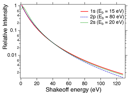
In the upper panel one sees a modest dependence of the spectral shape on principal quantum number , and a more dramatic dependence on . In the lower panel, an adjustment of is sufficient to produce a common spectral shape. We therefore use the 1s function for all relevant states, and allow both the binding energy and the normalization to be effective (fit) parameters. A similar strategy has been used by Saenz and Froelich Saenz and Froelich (1997) for molecular tritium, but here we are also assuming the scaling behavior persists to larger values of and . Introducing a leading constant
| (7) |
reduces correlations between the amplitude and scale factor of the shakeoff distributions. The intensity normalization is unity when the arbitrary constant . The Levinger distributions use a large-Z approximation, but serve our purpose here.
The shakeoff spectral distribution must be convolved with the Lorentzian width of the 2-hole state in question to produce the final shakeoff distribution,
| (8) |
Numerical convolution has been carried out successfully in test fits, but is computationally intensive inside a fitting procedure. A good approximation that is simpler is to take advantage of the narrow Lorentzian widths in comparison with the typical shakeoff widths. The convolution of a Lorentzian with a step is an analytic function, suggesting the following form:
| (9) |
wherein is replaced with so that can run over all non-zero values. Since we treat as a fit parameter, in general .
With these preliminaries, then, we have a complete listing of the positions of shakeup and shakeoff satellites, and moderate-resolution experimental spectra from which the optimized positions and intensities can be obtained. The original data are no longer available, and it was necessary to use software to read the points off the plots in Wark et al. (1991). Another source of conversion-line data is the work of Decman and Stoeffl Decman and Stoeffl (1990), but unfortunately it was not possible to recover analyzable data from the published plots.
To fit the spectrum, we used iminuit Ongmongkolkul (2012) for its ability to calculate the covariance matrix as well as minimize chi-squared values given constrained tunable parameters in a non-linear setting. The fit strategy is encapsulated in Table 3.
| Parameter ID | State | Uncertainty | Unit | |
| Intensity of shakeoff | ||||
| x1 | 9, 10 | -0.58 | 0.58 | % |
| x2 | 15 | -1.36 | 1.17 | % |
| x3 | 18, 19 | -0.18 | 0.18 | % |
| x4 | 22, 23 | -0.19 | 0.43 | % |
| Intensity of shakeup | ||||
| x6 | 1 – 8 | -0.47 | 0.47 | % |
| x7 | 11 – 14 | -1.11 | 0.74 | % |
| x8 | 16, 17 | -0.03 | 0.07 | % |
| x9 | 20, 21 | -0.05 | 0.05 | % |
| Binding Energy | ||||
| x11 | 1 – 10 | fixed | ||
| x12 | 11 – 15 | -1.3 | 1.3 | eV |
| x13 | 16 – 19 | -0.9 | 0.9 | eV |
| x14 | 20 – 23 | -5 | 5 | eV |
| Scale parameter | ||||
| x16 | 9, 10 | -0.5 | 0.6 | eV |
| x17 | 15 | -3.4 | 4.4 | eV |
| x18 | 18, 19 | -21 | 24 | eV |
| x19 | 22, 23 | -110 | 400 | eV |
The two spectra of Wark et al. (1991) were fit together to derive a consistent set of shakeup and shakeoff parameters. Points near the high-energy ends (11 in Fig. 1 and 5 in Fig. 2 of Wark et al. (1991)) were excluded because they could not be accurately read from the plots. The core peaks were fit with a Voigt profile to extract the instrumental width from the known natural width. The core peaks were found to be at 17822.67(4) and 900.48(4) eV, and the Gaussian instrumental widths were 23.17(7) and 6.48(12) eV FWHM, respectively. (The uncertainties are statistical only, and do not include calibration uncertainties.) The fits and residuals are shown in Figs. 2 and 3. The total is 710 for 241 degrees of freedom. As can be seen from the residual plots, the peak regions contribute non-statistically to . The final parameters therefore are obtained from fits restricted to eV in Fig. 1 and eV in Fig. 2 because of uncertainty in the instrumental line shape, as discussed below. Excluding the core peak regions, as indicated in the figures, has little effect on the shakeup and shakeoff parameter values themselves. The 4p shakeup intensity decreases by one standard deviation and other parameters change by a fraction of a standard deviation. The Gaussian parameters from the full fit are used in the restricted fit.
Fits to the shakeup and shakeoff regions yielded several local minima. They arise from ambiguity in assigning a spectral feature in the data to a corresponding theoretical one. The lowest , 200, assigned all the 4p strength to shakeup and none to shakeoff. That solution was rejected in light of the data of Picard et al. Picard et al. (1992), which show in the L-line spectra that the shake satellite is centered at 26 eV binding, not 20, and is therefore mainly shakeoff. Other minima in with values 213, 219, 223, and 225 placed the 3d shakeoff edge at 144 eV below the core state, which is inconsistent with Rb photoionization data Briggs (1981); Banna et al. (1978). The solution consistent with all known independent constraints had a minimum of 212. Given the 90+101 data points and 15 tunable parameters, per degree of freedom is 1.20.
As noted above, in the higher-resolution spectrum (Fig. 2 of Wark et al. (1991)), there are events in a region, the tail of the core peak, that should be devoid of states. The theoretical expectation that there are no 2-hole shakeup states within 20 eV of the core line is supported by the high-resolution data on photoionization of the 3d and 3p states in Kr reported by Eriksson et al. Eriksson et al. (1987), although earlier photoionization measurements by Spears et al. Spears et al. (1974) do show some weak intensity between 10 and 20 eV. The RDF theory is further supported in predicting the 4p shakeoff edge to be at 26.1 eV, in good accord with the ionization potential for the isoelectronic ion Rb II, 27.28 eV. The KATRIN internal-conversion data Altenmueller et al. (2020) cover the region within 15 eV of the 17.8-keV line and find it to be empty, and the Picard et al. Picard et al. (1992) spectra, particularly for the intense, narrow L3 line, show the 20-eV interval to be empty. Events in that region therefore imply that the instrumental response is not symmetrical and has a more intense low-energy tail than the high-energy one, which is well described by the Voigt profile. For this reason, the energy of the first 4p shakeup excitation has been fixed at 19.8 eV from the RDF prediction of Wark et al. (1991) (Table 2) because it cannot be reliably determined from this spectrum alone.
Similarly, in the lower-resolution data (Fig. 1 of Wark et al. (1991)) there is evidence that the peak shape deviates slightly from the Voigt profile. This is not unexpected, as the theoretical Darwin profile for crystal-diffraction monochromators is not the same as a Voigt profile, and may itself be modified by incidental effects such as heating.
It may be remarked that a different picture is seen in the Kr threshold 1s photoexcitation data of Deutsch and Hart Deutsch and Hart (1986). A rich and complex spectrum of weak satellites occupies the excitation region between 12.3 and 19.3 eV binding. These states consist of correlation and multiparticle satellites, states that would not be excited in the sudden approximation where the ejected electron has much higher kinetic energy than the binding energies. Such states fade to insignificant intensity at the energies imparted by internal conversion in 83Krm.


IV Results and conclusions
In Table 4 are summarized the parameters of the individual components that comprise the full shakeup and shakeoff spectrum of the K-32 line of 83Krm, and
| Final state | Intensity | Binding | Width | Scale | |
|---|---|---|---|---|---|
| , % | , eV | , eV | , eV | ||
| 0 | 2.70(6) | ||||
| 1 | 2.70(6) | ||||
| 2 | 2.70(6) | ||||
| 3 | 2.70(6) | ||||
| 4 | 2.70(6) | ||||
| 5 | 2.70(6) | ||||
| 6 | 2.70(6) | ||||
| 7 | 2.70(6) | ||||
| 8 | 2.70(6) | ||||
| 9 | 2.70(6) | 11.7 | |||
| 10 | 2.70(6) | 11.7 | |||
| 11 | 3.10(7) | ||||
| 12 | 3.10(7) | ||||
| 13 | 3.10(7) | ||||
| 14 | 3.10(7) | ||||
| 15 | 3.10(7) | 42.6 | |||
| 16 | 2.77(6) | ||||
| 17 | 2.77(6) | ||||
| 18 | 2.77(6) | 304 | |||
| 19 | 2.77(6) | 304 | |||
| 20 | 4.02(6) | ||||
| 21 | 3.93(9) | ||||
| 22 | 4.02(6) | 254 | |||
| 23 | 3.93(9) | 254 | |||
| 24 | 6.20(40) | ||||
| 25 | 3.81(6) | ||||
| 26 | 3.87(9) |
Fig. 5 shows the spectrum of the K-conversion line using the fitted parameters listed in the table.
The parameter uncertainties are included in Table 3. The uncertainties were obtained with the minos routine of iminuit that searches each parameter in turn for the change that increases by one, marginalizing over the others. In general the uncertainties are asymmetric. The correlation matrix determined from the Hessian is presented in Fig. 4. The largest element is -0.94 between the 4s shakeoff amplitude and the scale factor of 4p shakeoff.

The total intensity in shakeup and shakeoff below the core peak is found to be 34.7% of the core peak, in good agreement with the theoretical calculation (see Table 2). However, the fits confirm the observation Wark et al. (1991) that the RDF theory tends to overemphasize shakeup at the cost of shakeoff, even while conserving the total probability, for reasons that are at present not known. Moreover, the RDF calculations of Wark et al. (1991) overbind the 3d states by about 19 eV.
This work was motivated by the development of the cyclotron radiation emission spectroscopy (CRES) method, exemplified by Project 8 Asner et al. (2015). Electrons emitted from a radioactive gas (3H and 83Krm particularly) are trapped in a magnetic trap for a precise measurement of their cyclotron frequencies and, hence, energies. Electrons escape by scattering from background gas atoms, and several scatters are typically needed to eject the electron. The trap thus contains both scattered and unscattered electrons, an effect that must be taken into account in determining the instrumental response. The 83Krm lines provide an ideal testbed for this determination, but the shakeup and shakeoff satellites occupy the same region of the spectrum as scattered electrons, and therefore must be quantitatively treated.
The KATRIN experiment now in operation Aker et al. (2019) does not use 83Krm for a direct determination of resolution or scattering; an electron gun is used. The isotope is, however, brought to bear on a number of systematic tests either alone or mixed with tritium (see, for illustration, Belesev et al. (2008)). Even so, the satellite structure of the lines plays little role in the interpretation of those tests, and it is not expected that the results reported here will influence the KATRIN program greatly. KATRIN’s high statistical and systematic precision takes 83Krm out of the list of contributions to Eq. 1.
In summary, the shakeup and shakeoff spectrum derived in this work is intended to serve as an improved prediction of the extended shape of the 17.8-keV internal conversion line of 83Krm. The spectrum provided will find utility in currently running and planned tritium beta decay neutrino mass experiments, such as Project 8 Asner et al. (2015) and, possibly, KATRIN Angrik et al. (2005); Altenmueller et al. (2020). The spectrum also provides a baseline for further theoretical work. New high-resolution measurements of this spectrum by both internal conversion and photoionization are well within technical reach Glatzel et al. (2001) and are encouraged.
We gratefully acknowledge discussions with Christine Claessens and Gerald Seidler. This material is based upon work supported by the U.S. Department of Energy Office of Science, Office of Nuclear Physics under Award Number DE-FG02-97ER41020.
References
- Robertson et al. (1991) R. G. H. Robertson, T. J. Bowles, G. J. Stephenson Jr., D. L. Wark, J. F. Wilkerson, and D. A. Knapp, Phys. Rev. Lett. 67, 957 (1991).
- Stoeffl and Decman (1995) W. Stoeffl and D. J. Decman, Phys. Rev. Lett. 75, 3237 (1995).
- Kraus et al. (2005) C. Kraus, B. Bornschein, L. Bornschein, J. Bonn, B. Flatt, A. Kovalik, et al., Eur. Phys. J. C40, 447 (2005), eprint hep-ex/0412056.
- Belesev et al. (2008) A. Belesev, E. Geraskin, S. V. Zhuikov, B.L.and Zadorozhny, O. V. Kazachenko, V. M. Kohanuk, et al., Phys. Atom. Nucl. 71, 427 (2008), [Yad. Fiz. 71, 449 (2008)].
- Aseev et al. (2012) V. Aseev, A. Belesev, A. Berlev, E. V. Geraskin, A. A. Golubev, N. A. Lihovid, et al., Phys. Atom. Nucl. 75, 464 (2012), [Yad. Fiz. 75, 500 (2012)].
- Aker et al. (2019) M. Aker, K. Altenmüller, M. Arenz, M. Babutzka, J. Barrett, S. Bauer, et al. (KATRIN Collaboration), Phys. Rev. Lett. 123, 221802 (2019), URL https://link.aps.org/doi/10.1103/PhysRevLett.123.221802.
- Asner et al. (2015) D. Asner, R. Bradley, L. de Viveiros, P. Doe, J. Fernandes, F. M., et al. (Project 8), Phys. Rev. Lett. 114, 162501 (2015), eprint 1408.5362.
- Akerib et al. (2017) D. S. Akerib, S. Alsum, H. M. Araújo, X. Bai, A. J. Bailey, J. Balajthy, et al. (LUX), Phys. Rev. D97, 112009 (2017), eprint 1708.02566.
- Aprile et al. (2018) E. Aprile, J. Aalbers, F. Agostini, M. Alfonsi, L. Althueser, F. D. Amaro, et al. (XENON), Phys. Rev. Lett. 121, 111302 (2018), eprint 1805.12562.
- Kastens et al. (2009) L. W. Kastens, S. B. Cahn, A. Manzur, and D. N. McKinsey, Phys. Rev. C 80, 045809 (2009), URL https://link.aps.org/doi/10.1103/PhysRevC.80.045809.
- Robertson and Knapp (1988) R. G. H. Robertson and D. A. Knapp, Annu. Rev. Nucl. Part. Sci. 38, 185 (1988).
- Carlson and Nestor (1973) T. A. Carlson and C. W. Nestor, Phys. Rev. A 8, 2887 (1973), URL https://link.aps.org/doi/10.1103/PhysRevA.8.2887.
- Wark et al. (1991) D. L. Wark, R. Bartlett, T. J. Bowles, R. G. H. Robertson, D. S. Sivia, W. Trela, et al., Phys. Rev. Lett. 67, 2291 (1991), URL https://link.aps.org/doi/10.1103/PhysRevLett.67.2291.
- Picard et al. (1992) A. Picard, H. Backe, J. Bonn, B. Degen, R. Haid, A. Hermanni, et al., Z. Phys. A 342, 71 (1992).
- Vénos et al. (2018) D. Vénos, J. Sentkerestiová, O. Dragoun, M. Slezák, M. Ryšavý, and A. Špalek, JINST 13, T02012 (2018).
- Altenmueller et al. (2020) K. Altenmueller, M. Arenz, W.-J. Baek, M. Beck, A. Beglarian, J. Behrens, et al., J. Phys. G 47, 065002 (2020), eprint 1903.06452.
- Arenz et al. (2018) M. Arenz, W.-J. Baek, M. Beck, A. Beglarian, J. Behrens, T. Bergmann, et al., Eur. Phys. J. C 78, 368 (2018), ISSN 1434-6052, URL https://doi.org/10.1140/epjc/s10052-018-5832-y.
- Levinger (1953) J. S. Levinger, Phys. Rev. 90, 11 (1953), URL https://link.aps.org/doi/10.1103/PhysRev.90.11.
- Kikas et al. (1996) A. Kikas, S. Osborne, A. Ausmees, S. Svensson, O.-P. Sairanen, and S. Aksela, Journal of Electron Spectroscopy and Related Phenomena 77, 241 (1996), ISSN 0368-2048, URL http://www.sciencedirect.com/science/article/pii/0368204895025529.
- Deutsch and Hart (1986) M. Deutsch and M. Hart, Phys. Rev. Lett. 57, 1566 (1986), URL https://link.aps.org/doi/10.1103/PhysRevLett.57.1566.
- Briggs (1981) D. Briggs, Surface and Interface Analysis 3, v (1981), URL https://onlinelibrary.wiley.com/doi/abs/10.1002/sia.740030412.
- Banna et al. (1978) M. S. Banna, B. Wallbank, D. C. Frost, C. A. McDowell, and J. S. H. Q. Perera, J. Chem. Phys. 68, 5459 (1978), eprint https://doi.org/10.1063/1.435723, URL https://doi.org/10.1063/1.435723.
- Lederer and Shirley (1978) C. M. Lederer and V. S. Shirley, eds., Table of Isotopes (Wiley, 1978), 7th ed.
- Schaphorst et al. (1993) S. J. Schaphorst, A. F. Kodre, J. Ruscheinski, B. Crasemann, T. Åberg, J. Tulkki, et al., Phys. Rev. A 47, 1953 (1993), URL https://link.aps.org/doi/10.1103/PhysRevA.47.1953.
- Jänkälä et al. (2011) K. Jänkälä, M. Alagia, V. Feyer, K. C. Prince, and R. Richter, Phys. Rev. A 84, 053426 (2011), URL https://link.aps.org/doi/10.1103/PhysRevA.84.053426.
- Saenz and Froelich (1997) A. Saenz and P. Froelich, Phys. Rev. C 56, 2162 (1997), URL https://link.aps.org/doi/10.1103/PhysRevC.56.2162.
- Decman and Stoeffl (1990) D. J. Decman and W. Stoeffl, Phys. Rev. Lett. 64, 2767 (1990), URL https://link.aps.org/doi/10.1103/PhysRevLett.64.2767.
- Ongmongkolkul (2012) P. Ongmongkolkul (2012), URL {https://iminuit.readthedocs.io/en/latest/about.html}.
- Eriksson et al. (1987) B. Eriksson, S. Svensson, N. Märtensson, and U. Gelius, J. Phys. Colloques 48, 531 (1987).
- Spears et al. (1974) D. P. Spears, H. J. Fischbeck, and T. A. Carlson, Phys. Rev. A 9, 1603 (1974), URL https://link.aps.org/doi/10.1103/PhysRevA.9.1603.
- Angrik et al. (2005) J. Angrik, T. Armbrust, A. Beglarian, U. Besserer, J. Blümer, J. Bonn, et al. (KATRIN) (2005), URL http://bibliothek.fzk.de/zb/berichte/FZKA7090.pdf.
- Glatzel et al. (2001) P. Glatzel, U. Bergmann, F. M. F. de Groot, and S. P. Cramer, Phys. Rev. B 64, 045109 (2001), URL https://link.aps.org/doi/10.1103/PhysRevB.64.045109.