Sequential Routing Framework:
Fully Capsule Network-based Speech Recognition
Abstract
Capsule networks (CapsNets) have recently gotten attention as a novel neural architecture. This paper presents the sequential routing framework which we believe is the first method to adapt a CapsNet-only structure to sequence-to-sequence recognition. Input sequences are capsulized then sliced by a window size. Each slice is classified to a label at the corresponding time through iterative routing mechanisms. Afterwards, losses are computed by connectionist temporal classification (CTC). During routing, the required number of parameters can be controlled by the window size regardless of the length of sequences by sharing learnable weights across the slices. We additionally propose a sequential dynamic routing algorithm to replace traditional dynamic routing. The proposed technique can minimize decoding speed degradation caused by the routing iterations since it can operate in a non-iterative manner without dropping accuracy. The method achieves a 1.1% lower word error rate at 16.9% on the Wall Street Journal corpus compared to bidirectional long short-term memory-based CTC networks. On the TIMIT corpus, it attains a 0.7% lower phone error rate at 17.5% compared to convolutional neural network-based CTC networks [Zhang et al., 2016].
keywords:
Capsule network, Automatic speech recognition, Sequence-to-sequence, Connectionist temporal classification1 Introduction
Capsule networks (CapsNets) [Hinton et al., 2011, Sabour et al., 2017, Hinton et al., 2018] are a kind of neural networks that represent a specific entity type with a group of neurons called a capsule instead of a single neuron. The initial motivation of CapsNets was to abstract information explicitly by adapting an unsupervised clustering mechanism called routing-by-agreement between capsules, to conventional neural networks. Capsules can be trained to represent not only the existence of entity types but also entity instantiation parameters such as textures, angles, colors, etc. Thus, CapsNets can be regarded as architectures for inverse graphics [Sabour et al., 2017]. CapsNets have shown higher accuracy in image classification compared to convolutional neural networks (CNNs) [Sabour et al., 2017, Hahn et al., 2019, Malmgren, 2019]. Recently, researchers have focused more on adapting CapsNets for practical problems either by scaling their routing methods [Tsai et al., 2020] or by combining them with other architectures [He et al., 2019, Srivastava et al., 2019, Wang, 2019]. There are also attempts to apply CapsNets to classify sequence data [Bae and Kim, 2018, Iqbal et al., 2018, Wu et al., 2019].
Sequence to sequence (seq2seq) learning is an approach to learn mappings between sequences and is successfully implemented by neural models [Sutskever et al., 2014]. Connectionist temporal classification (CTC) [Graves et al., 2006] is a popular loss function in seq2seq problems. By adapting CTC to automatic speech recognition (ASR) systems, it became possible to learn the alignments between speech signal sequences and label sequences directly unlike the conventional hidden Markov model (HMM) deep neural network (DNN) based systems [Hinton et al., 2012] which needed alignments from an HMM Gaussian mixture model (GMM) system for training the DNN. CTC based ASR systems [Graves et al., 2006] were first built on long short-term memory (LSTM) [Hochreiter and Schmidhuber, 1997] networks. In order to accelerate training, CNN-based CTC networks [Zhang et al., 2016] were proposed. The newly proposed networks showed 2.5x increase in training speed while maintaining phoneme-level accuracies which requires relatively short-term dependencies. Transformer-based [Vaswani et al., 2017] ASR systems [Dong et al., 2018] were also proposed as a faster training model compared to recurrent seq2seq models by introducing self-attention. However, they require the whole context to compute self-attention maps for each time slice. Recently, online ASR systems based on Transformers have been researched [Moritz et al., 2020].
In ASR, speech feature sequences can be regarded as two-dimensional images with the time length as width and the feature coefficient dimension as height. We hypothesized that CapsNets can potentially have richer representation capabilities than CNNs in ASR since the same shapes in the feature sequences represent different pronunciations depending on their positions which can be more precisely learned by CapsNets [Hinton et al., 2011]. Moreover, like CNNs, CapsNets are trained by computing the derivatives of error functions by propagating errors backwards over layers rather than input sequences, i.e., the number of steps to compute the gradients are decided according to the number of layers regardless of the length of input sequences. Thus, given enough receptive fields, their layer-wise encoding is expected to alleviate the gradient vanishing and exploding problems that could arise when training long-term dependencies using recurrent neural networks (RNNs).
There have been attempts to apply CapsNets to seq2seq tasks in combination with other models [Srivastava et al., 2019, Wang, 2019], but the utilization of CapsNets could be maximized more. In addition to the computational burden due to the routing mechanism itself [Marchisio et al., 2020], there are hurdles in adopting existing CapsNets to seq2seq problems. This is because directly routing from input sequences to output sequences is problematic in the perspectives of both memory consumption and computational complexity. For the routing mechanism, prediction vectors representing all the paths from the lower-level capsules to the higher-level capsules are given as inputs, then each of them is weighted by the routing coefficient. Thus, the size of the transformation matrix to construct the vectors and the number of routing coefficients exponentially increase according to the length of input and output sequences. As a result, the memory requirements can exceed the acceptable size. Moreover, the computational burden resulting from the vector construction and the routing method can interfere with the real-time processing of ASR systems.
In this paper, we introduce the sequential routing framework (SRF) which is a novel method to build up CTC networks based on a CapsNet-only architecture. SRF is applicable to iterative routing-by-agreement methods [Sabour et al., 2017, Hinton et al., 2018] which update the routing coefficients of the current iteration using the outputs of the previous iteration in an expectation and maximization manner. We chose to apply dynamic routing (DR) [Sabour et al., 2017] to the framework since it has shown competitive accuracy and intuitive mechanisms compared to more recent architectures [Hahn et al., 2019, Malmgren, 2019]. To train SRF models, the input sequences are first converted to three-dimensional sequences through convolutional and linear projection layers. The encoded sequences are sliced by time windows and multiple routing iterations are performed for each slice to classify the corresponding label. By slicing capsule groups, the existing routing mechanisms for the fixed size data can be applied. In addition, the models are trained to use the limited context when encoding each frame, thus the proposed method can have online processing capabilities unlike the architectures that require a full-sequence as an input such as bidirectional LSTMs (BLSTMs) and Transformers. Afterwards, the training loss is calculated using CTC. The framework achieved competitive accuracy while minimizing decoding speed degradation and required parameters by sharing two types of information during routing across the slices. First, the transformation matrices are shared so that only the fixed size of parameters is required regardless of input lengths. Moreover, the capsule clustering information is also conveyed to the next slice by initializing routing coefficients of the current slice based on the previous routing results. As a result, only one routing iteration is required for each slice meanwhile the routing coefficients are updated by the number of times corresponding to the each slice index.
The clear contribution of this study is that, to the best of our knowledge, SRF is the first CapsNets only architecture for seq2seq speech recognition. The proposed method achieved competitive performance on speech recognition in terms of accuracy and online processing capability by sharing the learnable weights and the clustering information.
2 Preliminaries
2.1 CTC loss function
A CTC network [Graves et al., 2006] is defined as a continuous map from an dimensional input sequence of length to the same length sequence of dimensional probability vectors with parameters . is the cardinality of an expanded label set consisting of the union between the label symbol set and a blank symbol, blank. This network contains a softmax layer at the top of it in order to convert logits to valid probability distributions. The softmax layer for a given vector is computed as follows:
| (1) |
, where is the -th element of . CTC computes a conditional probability of a label sequence for a given input sequence by summing up every conditional probability of possible paths , i.e., . The possible paths are computed using an inverse of a map from an expanded label sequence to . performs many-to-one mappings by simply removing repeating and blank symbols from the given paths. For example, (“cc-aaa-tt”) = (“-cc-aattt”) = “cat”, where “-” indicates a blank symbol. It allows CTC networks to learn alignments solely from the input and output sequence pairs. A conditional probability of each possible path is computed as , where is an expanded label symbol in a path at time and is the -th feature vector of . The CTC loss is defined as a negative of the summation of the log probabilities of all CTC paths. The gradients are computed by differentiating the probability function using the CTC forward-backward algorithm, which is a kind of dynamic programming.
2.2 Capsule Network
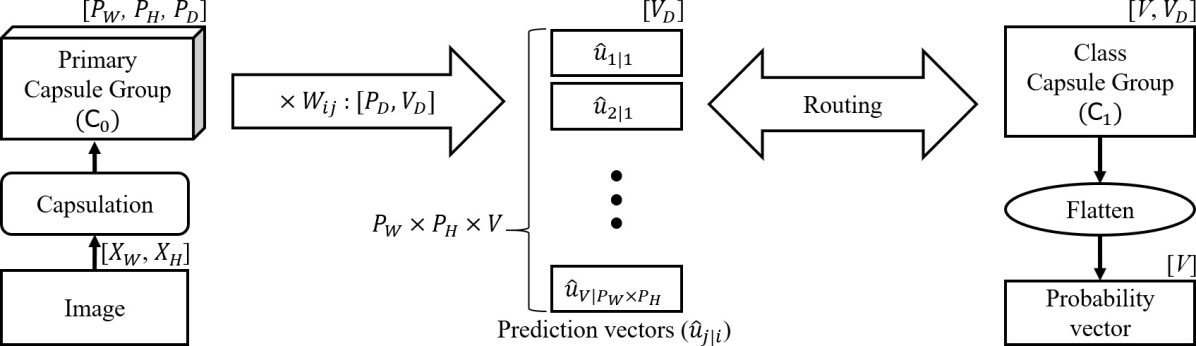
A CapsNet [Hinton et al., 2011, Sabour et al., 2017, Hinton et al., 2018] for a two-dimensional data classification problem is defined with the parameter as a map, , which maps an input data of size to a -dimensional probability vector, e.g., and represent the width and height of the two-dimensional input images respectively as shown in Fig 1. In the figure, the dimension above each capsule group block indicates the dimension of a group of instantiation parameter vectors. To initiate the routing method, the input is converted to a capsule group, . In the capsulation process, and are converted to the width and the height of the lowest capsule group respectively. Thus, consists of a pair of an activation group, , and a group of instantiation parameter vectors, , where is the dimension of parameter vectors of capsules in the lowest level. can be computed either from [Sabour et al., 2017] or from additional neural layers [Hinton et al., 2018]. Routing iterations are performed between the higher-level capsules and the prediction vectors , each of which represents a path from the -th lower-level capsule to the -th higher-level capsule. Thus, in Fig 1, the range of and are and respectively. is computed by multiplying an instantiation parameter of the -th lower-level capsule with a transformation matrix . During the training process, for a certain entity type, each of the elements of and can be trained to represent an existence probability and characteristics respectively [Hinton et al., 2011]. Accordingly, CapsNets can potentially [Lenssen et al., 2018] represent invariance of the existence probabilities and also equivariance of the properties of the entity type.
The groups in the lowest, highest, and in-between levels are called as primary, class, and convolutional capsule groups respectively. In this paper, for the sake of brevity, we describe the structure of as the structure of the capsule group because the structure of can be derived by removing the dimension from the structure of . The first and second dimensions of the class capsule groups are and respectively, and their activation groups are the outputs of the CapsNets, i.e., the CapsNets output -dimensional vectors. Gradient based learning methods used for conventional neural networks are applicable. A key procedural difference of CapsNets is that they filter information flow using routing-by-agreement.
2.2.1 Dynamic Routing
DR [Sabour et al., 2017] is an iterative routing-by-agreement method which works in a non-parametric expectation and maximization manner based on the similarities between capsules. In this section, in order to distinguish instantiation vectors in the lower- and higher-level, we use and respectively. We also use and to represent the index of the vectors in lower- and higher-levels respectively. The -th activation scalar is computed by the length of the -th instantiation vector as follows:
| (2) |
In order to normalize to a valid probability, a nonlinear function, which is referred to as a squash function, is defined as follows:
| (3) |
, where is a unnormalized instantiation parameter vector for the -th capsule in the higher-level. This function also has a role to make the activations more discriminative by pushing most of the values to around zero or one. A prediction vector, , is computed as . The vector indicates a path from the -th capsule in the lower level to the -th capsule in the higher level. A transformation matrix, , is the only required parameter matrix for the routing mechanism. A , iteration number and level index are given for DR. is ranged from 0 to for a CapsNet consisting of layers, i.e., of primary capsules is 0. The primary capsules are calculated through multiple convolutional layers. Routing coefficients are zero-initialized, i.e., coupling coefficients are uniformly initialized. Then is updated to maximize the agreements between and as in Algorithm 1.
3 Sequential Routing Framework

SRF is an iterative routing framework for sequence data and it is defined as a modified version of the original CapsNets with the parameter , , from a real valued feature sequence having a length and a feature dimension to a dimensional probability vector sequence of a width as shown in Fig. 2. The shapes of an input, output sequence and each capsule group are written above the boxes in the diagram. A two-dimensional input feature sequence is transformed into a primary capsule group , whose width, height and depth are , and respectively, through a capsulation block. Afterwards, is fed into the lowest capsule layer, then encoded to a convolutional capsule group , whose width, height and depth are , , and respectively. For the sake of brevity, we describe all the convolutional capsule groups have the same shape. A class capsule group has , , and as width, height and depth respectively. It is flattened to an activation vector sequence, i.e., , which is a sequence of probability vectors where each element indicates a probability of observing a corresponding label symbol. Finally, the CTC loss between and a label sequence is computed.
3.1 Capsulation
Capsulation is a neural layer block that converts from to , as shown in Fig. 3. has the structure of width and height and the structure of has the dimension in addition to the two dimensions of . The layers to compute are optional structures depending on the routing mechanism. is first encoded into three-dimensional representation with width , height and depth through two-dimensional convolutional layers, where and . We employed maxout [Goodfellow et al., 2013] as activation functions of the convolutional layers because of their competitive accuracy in ASR [Zhang et al., 2016]. Thus, the -th convolutional layer in the first sub-block is defined as follows:

| (4) |
, where is a convolutional operator, is the number of convolutional operations in a layer and is the dropout rate. indicates a convolution weight matrix for the -th channel of the -th convolutional operation in the -th layer. The -th is an input sequence, i.e., . For all the cases, we set and to 2 and 0.2 respectively. Subsequently, the output sequence is flattened to by reshaping it to width and height , then it is fed into two different layer blocks. They are projected to a normalized vector sequence, i.e., an activation group , with width and height , through a nonlinear layer as follows:
| (5) |
, where is a learnable weight matrix and is a nonlinear function for normalizing the values. They are also projected to another representation having the same shape with as follows:
| (6) |
, where is a learnable weight matrix. Afterwards, is converted to by expanding their channel dimensions into through a two-dimensional convolutional layer activated with the maxout function as follows:
| (7) |
, where indicates a convolutional weight matrix for the -th output channel of the -th convolutional operation.
3.2 Routing-by-agreement for sequence to sequence learning
In SRF, in order to adapt the existing routing methods with minimal changes and to control the required size of parameters regardless of the length of input sequences, each subgroup of a capsule group, is sliced by without overlapping adjacent slices, i.e., . In order to expand a receptive field on , sequential routing is performed between windows of the time slices in the lower level, which consist of the consecutive slices, and single slices in the higher level. The bottom box in Fig. 2 describes an example of sequential routing between the window () centered on -th slice in the lower level and the -th slice in the higher level. In this study, we set the stride of the sliding window to one in all the cases and the both side of window contexts beyond the sequence boundaries are padded as zero. Thus when is set to 1, the routing iteration is performed times for a capsule group having width . The receptive field on is computed as for each slice of . Accordingly, online decoding is allowed with a time delay corresponding to , where is the right context size of the window. In each capsule layer, the -th prediction vector is calculated from the -th instantiation vector through a linear transformation using as follows:
| (8) |
, where and are heights of lower and higher capsule groups respectively. of the first layer and of the last layer are the and respectively. The two heights are in-between layers. Accordingly, each has the shape of the product of depths of lower and higher capsule groups. are shared across all the time slices. Therefore, the number of parameters for the routing mechanism in a layer is controlled only by the shape of capsule groups and .


We have an assumption that consecutive slices in sequence data have similar properties. Based on that, we designed an iterative routing mechanism which initializes routing coefficients for the -th slice based on the routing output of the -th slice. Fig. 4 is a schematic diagram of the two different iterative routing mechanisms of and for three consecutive slices. In this figure, the three dimensional block represents the routing procedures, is an iteration index in the range between 1 and , and the dashed and solid arrows describe the optional and required flows respectively. In the original version of routing, is initialized uniformly, then updated within each iteratively as in Fig. 4a in the order of a maximization and an expectation stage. The expectation stage means to update to improve the agreements between adjacent capsule groups and the updated coefficients are applied in the maximization stage. Thus, if is set to 1, output capsule groups are computed using the uniform in the original routing method. The proposed sequential routing method has two procedural differences as described in Fig. 4b. First, is initialized based on the agreement between the routing output of the previous time slice and the current routing input thus is uniformly initialized only at . The second procedural difference is the sub-procedure order of the routing mechanism which expects the initial before the first maximization stage. These two modifications make a similar effect of updating times to compute when . In other words, they alleviate the need for iterative updates of within each slice as an option. Consequently, decoding can be performed in a non-iterative way while minimizing accuracy degradation.
Sequential version of DR (SDR) works as Algorithm 2 for each between the -th and -th level. To explain the algorithm, we use the notations , , and their indices and respectively as explained in Section 2.2.1. is zero-initialized at . The expectation-maximization clustering is performed from line 5 to 11. At line 7, is updated by accumulating the agreements between and . To maximize the agreements, is computed as the summation of over all by weighting with the updated at line 9. The number of operations of an iteration remains the same as Algorithm 1 since only the order of the sub-procedures is changed.
4 Results
All evaluations were performed with the same settings when it comes to training CapsNets unless otherwise noted. Variables are initialized using a fan-avg method [Glorot and Bengio, 2010] from the uniform distribution, i.e., learning weights are drawn from , where is the average of the input and output unit numbers and the scaling factor is set to 1.0. For all SRF models, dropout [Srivastava et al., 2014] layers are applied after every layer at rate 0.2. We utilized two types of normalization layers. First, batch normalization [Ioffe and Szegedy, 2015] layers are added after every convolutional layer in the first convolutional sub-block of a capsulation block. Second, layer normalization [Ba et al., 2016] layers are also applied between every capsule layer. One modification is that layer normalization is performed not for each capsule but over all capsules in the same time slice. An Adam optimizer [Kingma and Ba, 2015] is used for the gradient descent algorithm. A learning rate is updated for each step depending on the two hyper-parameters which are a warming-up step and a scaling factor as follows:
| (9) |
The beam size for decoding is set to 100. The proposed method was implemented with Tensorflow [Abadi et al., 2016]. The error rates were evaluated with SCTK111https://github.com/usnistgov/SCTK.
4.1 The TIMIT Corpus
TIMIT [Garofolo et al., 1993b] consists of mono-channel read speech sampled at 16Khz. The training and test set consist of 4,620 utterances recorded from 462 speakers and 1,680 utterances recorded from 168 speakers respectively. We used a training set consisting of 3,696 utterances where all dialect utterances, i.e., the utterances tagged as “SA”, were removed and used 192 sentences from the core test set recorded from 24 speakers. A validation set was selected from another portion of the test set and was made up of 400 utterances recorded from 50 different speakers. A total of 63 labels consisting of 61 phonemes plus a padding and blank symbol were used during both training and decoding. At the top layer, the values in which route to a class capsule corresponding to the padding symbol are masked as zero. To evaluate phoneme error rates (PERs), the phoneme labels were mapped to 39 labels [Lee and Hon, 1989]. The features were extracted with a 10 ms hop size and 25 ms window size, and were encoded with 40-dimensional Fourier-transform-based filterbanks plus energy. Their temporal first and second-order differences were added with the delta-window size 2, thus 123-dimensional vectors were used as inputs. The input features were normalized to zero mean and unit variance per-speaker. The data splitting and feature extraction were performed using Kaldi222https://github.com/kaldi-asr/kaldi[Povey et al., 2011].
The learning schedule, is set to 1,200. We applied an additional decay policy where the learning rate was started by setting to 0.5, and then was reduced to 0.1 after 27 epochs. The models were trained for 200 epochs to ensure sufficient weight updates. In order to avoid the accuracy being dependent on the early stop time, we evaluated PERs with a model which is the averaged checkpoint of the last 10 epochs. Approximately 5K frames are contained in a batch for each training step according to their sequence length thus the learnable weight are updated 42K times per experiment. We first investigated the performance gain from the proposed routing algorithm using small CapsNet models with and .
| Routing | Iteration | PER(%) | |
|---|---|---|---|
| Method | Valid | Test | |
| DR | 1 | 25.6 | 26.8 |
| 2 | 25.4 | 26.6 | |
| 3 | 25.4 | 26.8 | |
| SDR | 1 | 24.4 | 25.5 |
| 2 | 24.3 | 25.7 | |
| 3 | 24.5 | 25.8 | |
We compared SDR with DR as in Table 1. and the depth of capsule groups are set to 1 and 8 respectively. Accordingly, the total number of parameters of each model is 207,682. In each of the two cases, statistically significant differences in PERs depending on the number of iterations are not observed. However, in all the cases, SDR shows about 1% lower PERs than that of DR. These experiments will be further analyzed in Section 5 by investigating the heat maps of .
| Window () | Look-ahead | Delay | Params. | Valid(%) | Test(%) | |||
|---|---|---|---|---|---|---|---|---|
| frames | (ms) | (M) | PER | EOS | PER | EOS | ||
| 0 | 0 | 11 | 122.5 | 0.21 | 24.4 | 52.8 | 25.6 | 55.7 |
| 1 | 0 | 11 | 122.5 | 0.30 | 23.8 | 25.5 | 25.1 | 26.6 |
| 1 | 1 | 15 | 162.5 | 0.39 | 21.8 | 66.5 | 23.7 | 69.3 |
| 2 | 0 | 11 | 122.5 | 0.39 | 23.3 | 27.5 | 24.5 | 26.6 |
| 2 | 1 | 15 | 162.5 | 0.48 | 22.5 | 53.0 | 23.6 | 53.1 |
| 2 | 2 | 19 | 202.5 | 0.57 | 20.2 | 99.8 | 21.7 | 100.0 |
| 3 | 2 | 19 | 202.5 | 0.66 | 20.8 | 94.0 | 21.9 | 93.8 |
| 4 | 1 | 15 | 162.5 | 0.66 | 21.1 | 84.5 | 22.6 | 81.3 |
| 5 | 0 | 11 | 122.5 | 0.66 | 22.3 | 32.5 | 23.9 | 32.3 |
We evaluated SRF models according to the configurations of as in Table 2. Their and capsule group depths are set to 1 and 8 respectively. As is expanded from 1 to 6, the numbers of required parameters (Params.) are increased from 0.21 to 0.66 million (M) as explained in Section 3.2. With the consideration of algorithmic delay caused by , all models are set to have either longer than or equal to . The time delays were estimated by “hop size (10ms) look-ahead frames + 12.5ms (the half of window size 25ms)”. The number of look-ahead frames includes 4 more frames in addition to the frames for the setting of due to computing the delta plus double-delta features. The relative PER reductions (RPERRs) are at most 17.2% and 15.2% for Valid and Test respectively depending on . End-of-sentence (EOS) detection rates seem to be one of the reasons why the settings that have unbalanced contexts show worse PERs than settings with balanced contexts since the detection rates show a large range from about 26% to 100% for both sets according to the setting of .


The relationship between the configuration of the window (X-axis) and PERs (Y-axis) are more explicitly described in Fig. 5. “2-1” indicates that and are 2 and 1 respectively. Blue triangles and orange circles indicate Valid and Test respectively in Fig. 5a. In the figure, the three evenly sliced cases which are “0-0”, “1-1” and “2-2”, show almost linear error reductions according to for the both sets. We can also see multiple cases where the balance of and has more of an effect on lowering the PERs than the number of parameters when . These phenomena are described by the dashed arrows in the figure and the percentages beside the arrows are RPERRs between the balanced and unbalanced window configurations. The models “1-1” and “2-0” have the same receptive field, but the model “1-1” shows relatively 6.4% and 3.3% lower PERs for Valid and Test respectively. In addition, although the model “2-1” has wider receptive field compared to the model “1-1”, it only shows slightly lower PER (relatively 0.4%) on Test but relatively 3.1% higher PER on Valid. Even more, the “5-0” model shows relatively about 9% worse PERs than the “2-2” model on the both evaluation sets. As of models (X-axis) expands, the EOS detection rates (Y-axis) get higher as shown in Fig. 5b. The detection rates are the averages from the two evaluation sets. The models which have one longer which are “1-0”, “2-1” and “3-2”, show lower EOS detection rates than that of “0-0”, “1-1”, and “2-2” respectively. As the differences between both sides of the window context size get bigger, the PERs and EOS detection rates of the settings get worse, i.e., phone recognition rates (PRRs) and EOS detection rates of the settings show the relationships such as “5-0” “4-1” “3-2” with the same number of parameters.
| Depth | Params. | PER(%) | |
|---|---|---|---|
| (M) | Valid | Test | |
| 2 | 0.14 | 26.6 | 27.9 |
| 4 | 0.19 | 23.7 | 25.0 |
| 8 | 0.39 | 21.8 | 23.7 |
| 16 | 1.15 | 20.6 | 21.9 |
We also evaluated PERs by doubling the capsule group depth continually from 2 to 16, as in Table 3. In these experiments, and are fixed to 1, and is set to 1. The required parameters are increased nearly proportional to the depth of capsules from 0.14M to 1.15M as explained in Section 3.2. The RPERRs between the depth 2 and 16 cases for Valid and Test are 22.6% and 21.5% respectively. The PER reduction for both sets is 2.9% when increasing the depth from 2 to 4. Meanwhile, when increasing the depth from 4 to 8, it decreases to less than 2.0%, even though the increase in the number of parameters is 4 times larger from 0.05M to 0.2M.
| Model | Look-ahead | Delay | Params. | PER(%) | |
|---|---|---|---|---|---|
| frames | (ms) | (M) | Valid | Test | |
| BLSTM-5L-250H | Full | Full | 6.80 | - | 18.4 |
| ULSTM-3L-421H | 4* | 52.5* | 3.80 | - | 19.6 |
| CNN-10L-Maxout | 24* | 252.5* | 4.30 | 16.7 | 18.2 |
| TF-5L | Full | Full | 1.99 | 18.9 | 19.9 |
| TF-10L | Full | Full | 3.63 | 18.0 | 19.1 |
| TF-20L | Full | Full | 6.93 | 17.5 | 18.6 |
| SRF-1L | 15 | 162.5 | 1.01 | 20.1 | 21.5 |
| SRF-2L | 19 | 202.5 | 0.99 | 18.8 | 20.2 |
| SRF-5L | 31 | 322.5 | 1.58 | 16.5 | 18.1 |
| SRF-7L | 39 | 402.5 | 1.97 | 15.9 | 17.5 |
We compared the SRF models with other architectures as in Table 4. The referenced PERs were evaluated using LSTM[Graves et al., 2013] and CNN[Zhang et al., 2016]-based CTC networks. We also compared with Speech-Transformer [Dong et al., 2018]-based CTC networks which we implemented. The models have the following structures below.
- BLSTM-5L-250H* [Graves et al., 2013]: BLSTM(250, concat)5-FC(63)
- ULSTM-3L-421H* [Graves et al., 2013]: ULSTM(421)3-FC(63)
- CNN-10L-Maxout* [Zhang et al., 2016]: Conv(35, 64)-MP(31)-Conv(35,
64)3-Conv(35, 128)5-Conv(35, 24)-FCMO(512)2-FCMO(63)
- TF-5/10/20L: CNNFE-FCPE(128)-TF(128, 4, 1024)L-FC(63)
- SRF-1/2/5/7L: CNNFE-FC(60)-Conv(33, 8)-SDR(30, 8)(L-1)-SDR(63, 8)
* Estimated by considering the number of model parameters.
Each layer is defined as the list below.
- BLSTM(cell states, merge mode={concatenation (concat) or average (ave)}): a
BLSTM layer
- ULSTM(cell states): a unidirectional LSTM (ULSTM) layer
- Conv(filter size=frequencyframe, output channels, stride=[frequency=1,
frame=1]): a two dimensional convolutional layer activated with maxout,
the number of feature maps is twice of the channels.
- CNN frontend (CNNFE): Conv(33, 64, [2, 2]) 2
- MP(pooling size=frequencyframe): a max pooling layer
- FC(output dimension): a fully connected layer
- FCPE(output dimension): a fully connected layer + positional encoding
[Dong et al., 2018]
- FCMO(output dimension): a fully connected layer activated with maxout,
the number of units is twice of the dimensionality of output space.
- TF(embedding dimension, attention heads, inner layer size): a Transformer
encoder layer [Dong et al., 2018]
- SDR(, depth of the output capsule group, [=1, =1], =1): a SDR layer
is set to 0.13 and reduced to 0.04 under the same condition as in the cases of the CapsNets and is set to 1,000. There are approximately 15K frames in a batch according to the length of utterances. We set dropout rates for the inputs, attention heads, inner layers and residual connections to 0.3, 0.3, 0.4, and 0.4 respectively. Bigger penalties are added to non-diagonal elements in attention maps before applying the softmax function Eq. 1, depending on the distance from the diagonal of the maps in the form of as used in [Dong et al., 2018], where the scaling factor were set to 1.0. TF-5L contains a similar number of parameters as the biggest SRF model SRF-7L.
As the layers of SRF models are stacked up, the receptive fields are increased from 31 to 79 frames. The reason why SRF-1L requires 0.02M more parameters than SRF-2L is that SRF-1L directly connects primary capsule groups to class capsule groups thus SRF-1L needs 11,340 (60 63 3) transformation matrices while SRF-2L needs 11,070 ((60 30 + 30 63) 3). When comparing the two models, the number of layers seems to be more effective for reducing PERs than the number of parameters. Among the CTC networks except for SRF models, CNN-10L-Maxout [Zhang et al., 2016] shows the lowest PERs. Compared to CNN-10L-Maxout, although SRF-5L and SRF-7L require more delays, SRF-5L shows similar PERs with 63.3% fewer parameters. Moreover, SRF-7L achieves PERs of 15.9% and 17.5% for Valid and Test respectively, which are about 0.7% lower in PERs for both sets than that of CNN-10L-Maxout, with less than half of the parameters.
| Model | Params. | Training time | Decoding time | ||
| (M) | (in secs.) | Secs. | xRT | ||
| TF-5L | 1.99 | 12 | 12 | 0.02 | 0.90 |
| TF-10L | 3.63 | 13 | 13 | 0.02 | 0.93 |
| TF-20L | 6.93 | 17 | 16 | 0.03 | 0.93 |
| SRF-1L | 1.01 | 98 | 14 | 0.02 | 0.96 |
| SRF-2L | 0.99 | 98 | 17 | 0.03 | 0.97 |
| SRF-5L | 1.58 | 168 | 25 | 0.04 | 0.98 |
| SRF-7L | 1.97 | 215 | 32 | 0.06 | 1.00 |
We measured the training and decoding time of TF-5/10/20L and SRF-1/2/5/7L on a NVIDIATM RTX-3090 as in Table 5. The training time is in seconds to finish one epoch of training. The size of the train-batch is set to 10K frames so that gradients were updated 107 times. We evaluated the decoding time in seconds and real-time factors (xRT) with Test. SRF-7L requires 18.6 times longer training time compared to TF-5L which has the same number of parameters. The training time of SRF models is increased as the size of models get bigger. On the other hand, decoding time is increased as more layers are stacked up. The correlation coefficients () between SRF-7L and other models are larger than 0.90 in all the cases.
4.2 The Wall Street Journal Corpus
| Model | Look-ahead | Delay | Params. | WER(%) | |
|---|---|---|---|---|---|
| frame | (ms) | (M) | dev-93 | eval-92 | |
| BLSTM-5L | Full | Full | 21.11 | 23.4 | 18.0 |
| ULSTM-5L | 7 | 82.5 | 21.15 | 33.7 | 27.4 |
| CNN-10L | 87 | 882.5 | 21.12 | 33.7 | 26.9 |
| CNN-15L | 127 | 1282.5 | 21.08 | 30.1 | 24.7 |
| TF-20L | Full | Full | 21.13 | 25.4 | 21.6 |
| SRF-7L-Small | 67 | 682.5 | 7.75 | 26.4 | 20.3 |
| SRF-7L-Big | 67 | 682.5 | 15.45 | 25.3 | 19.4 |
| SRF-10L-Small | 91 | 922.5 | 10.51 | 23.4 | 18.6 |
| SRF-10L-Big | 91 | 922.5 | 21.13 | 22.4 | 16.9 |
The Wall Street Journal (WSJ) corpus [Garofolo et al., 1993a, Consortium and Group, 1994] contains mono-channel read speech sampled at 16Khz. The si284 data set, which consist of about 81-hours of transcribed audio data (37,416 utterances), was set for training. The dev-93 (503 utterances, 1.1 hours) and eval-92 (333 utterances, 0.7 hours) data set were used respectively to validate and evaluate the models. For both training and evaluations, a total of 32 labels which consist of 26 uppercase letters, noise marker, apostrophe, space, EOS symbol plus a padding and blank symbol was used. The feature extraction and training configuration are the same as used in Section 4.1 unless it is specified. When it comes to the learning schedule, was set to 25,000. of each model was individually set according to their valid loss curves and was halved at the 71st epoch out of 80 epochs. There were approximately 20K frames in a batch thus the weights were updated 110K times. Word error rates (WERs) were evaluated by averaging the last 5% of checkpoints (4 checkpoints). As in Table 6, the SRF models are compared with other CTC-based ASR systems which we implemented. The number of parameters of the compared models are set to 21.1M. The models in Table 6 were constructed as the list below:
- BLSTM-5L: CNNFE-BLSTM(441, ave)5-FC(32)
- ULSTM-5L: CNNFE-ULSTM(662)5-FC(32)
- CNN-10L: CNNFE-Conv(35,140)4-Conv(35, 300)5-Conv(35, 66)-
FCMO(1024)2-FCMO(32)
- CNN-15L: CNNFE-Conv(35, 100)4-Conv(35, 215)10-Conv(35, 66)-
FCMO(1024)2-FCMO(32)
- TF-20L: CNNFE-FCPE(256)-TF(256, 4, 1488)20-FC(32)
- SRF-7/10-Small: CNNFE-FC(52)-Conv(33, 16)-SDR(26, 16, [2, 2])(L-1)-
SDR(32, 16, [2, 2])
- SRF-7/10-Big: CNNFE-FC(60)-Conv(33, 20)-SDR(30, 20, [2, 2])(L-1)-
SDR(32, 20, [2, 2])
The dropout rates of both LSTM networks are set to 0.3 and 0.4 for input data and in-between layers respectively. The dropout rates are set to 0.2 between layers for both CNN models. The layer normalization [Ba et al., 2016] layers are added after every layer in both the LSTM and CNN-based CTC networks. The learning rates for BLSTM-5L and ULSTM-5L were set to 1e-4 and 5e-5 respectively without learning rate scheduling Eq. 9. The initial of other models was set to 0.6. For TF-20L and SRF-7L-Big, it decreased to 0.06 and 0.1, respectively. Besides the two models, was initially decreased to 0.5 and then to 0.1. SRF-10L-Big attains the lowest WER at 16.9% for eval-92 which is 1.1% better than that of BLSTM-5L. SRF-7L-Small requires almost half of the delay compared to CNN-15L and shows 7.3% and 7.1% lower WERs in dev-93 and eval-92 respectively compared to ULSTM-5L. SRF-10L-Small shows lower WERs with 68.0% of the parameters compared to SRF-7L-Big but it requires a 240 ms longer delay. Compared to TF-20L, relative WER reductions (RWERRs) of SRF-10L-Small are 7.9% and 13.9% for dev-93 and eval-92 respectively with half of the parameters.
| Model | Params. | Training time | Decoding time | ||
| (M) | (in secs.) | Secs. | xRT | ||
| BLSTM-5L | 21.11 | 1,414 | 31 | 0.01 | 0.96 |
| ULSTM-5L | 21.15 | 1,030 | 30 | 0.01 | 0.96 |
| CNN-10L | 21.12 | 2,143 | 24 | 0.01 | 0.94 |
| CNN-15L | 21.08 | 2,310 | 26 | 0.01 | 0.94 |
| TF-20L | 21.13 | 880 | 29 | 0.01 | 0.91 |
| SRF-7L-Small | 7.75 | 20,814 | 112 | 0.05 | 0.99 |
| SRF-7L-Big | 15.45 | 31,406 | 112 | 0.05 | 0.99 |
| SRF-10L-Small | 10.51 | 28,271 | 153 | 0.06 | 0.99 |
| SRF-10L-Big | 21.13 | 51,666 | 153 | 0.06 | 1.00 |
As in Table 7, we evaluated the training and decoding time of the models explained in Table 6 on a NVIDIATM RTX-3090. The size of train-batch was set to 7K frames thus gradient updates were performed 4,155 times for an epoch of training. The decoding time was measured using eval-92. To finish an epoch of training, SRF-10L-Big takes 59 times longer than TF-20L, which has the shortest training time, and 37 times longer than BLSTM-5L, while showing similar word recognition accuracy. As the parameters and layers of the SRF models increase, their training and decoding time increase respectively. between SRF-10L-Big and other models is at least 0.91.
5 Analysis

In this section, we investigate how the routing method works in SRF by observing the heat maps of for a 5.47 seconds length utterance (id: MNJM0_SI950) in the test set. In the heat maps, brighter cells refer to larger values ranging from 0.01 to 0.05. All models explained in this section are the same as explained in Table 1 of Section 4.2. Fig. 6 is a heat map of which maps from primary capsules (vertical-axis) to class capsules (horizontal-axis) of the iteration 1 version of the SDR model at . A corresponding reference label is the red circled symbol “h#”, which indicates the end of a sentence. The numbers on the vertical-axis indicates primary capsule indexes. The bar graphs at the bottom of the figure represents the summation of coefficients per each class capsule. The summation of each row, i.e., the summation of coefficients per each primary capsule, is one and the coefficients which route capsules to the padding symbol are masked to zero as explained in Section 3.2 and they are not represented in the heat map. As shown in the figure, primary capsules are mostly routed to a class capsule corresponding to a “pau” symbol with the accumulated coefficient of 0.52 then followed by “h#” with that of 0.41 and “blank” with that of 0.39. 7 primary capsules indexed by in the order of 17, 19, 20, 6, 7, 12 and 5 are routed more to the class capsule corresponding to the correct symbol “h#” rather than the capsule for “pau”.

We compare 25 heat maps for different iteration numbers from 1 to 3 between DR and SDR as in Fig. 7. The coefficients of iteration 1 version of DR are all the same so it is not included in the figure. The reference symbols for each are written in the bottom of the figure with the time markers. The majority of primary capsules are routed to the class capsule corresponding to the correct symbol. Among the two DR cases, the heat maps of the iteration 3 versions have a slightly higher contrast than that of the iteration 2 versions as shown in Fig. 7. In other words, as the number of iterations increases, it seems that the distributions become less uniform. The iteration 2 and 3 version of SDR models display the same phenomenon as the DR version. However, the SDR model with iteration 1 seems to have different behaviors besides that is uniform at . The model routes the capsules to “pau” more than any other version at . Moreover, at , i.e., the end of the sentence, the model seems to route the majority of capsules to the class capsules corresponding to “pau” rather than the correct symbol “h#” as explained earlier in this section.


In order to see how the phenomenon affects alignment, we checked the 10 probability vectors each at the beginning and end of the sentence as shown in Fig 8. Symbols are represented with different line shapes described in the right side of the figure. The labels on the X-axis of each graph indicate a symbol with the highest probability, i.e., the phoneme sequence of the greedy decoding. Reference time markers and symbols are written at the bottom of Fig 8a and Fig 8b. For all the cases, the misalignment phenomenon of the iteration 1 version of SDR model is not observed. It is not a big difference, but rather, the SDR model recognizes the symbol “s” as fast as the iteration 2 version DR as shown in Fig 8a. The EOS symbol “h#” is also precisely recognized in all the cases as in Fig 8b. Even in the case of SDR when iteration is set to 1 at , unlike the heat map where most of the primary capsules are routed to the class capsule to the symbol “pau”, the probability of “h#” is the largest.
| Routing | Iteration | Edit distance rate (%) | |
|---|---|---|---|
| Method | Valid | Test | |
| DR | 2 | 0.14 | 0.14 |
| 3 | 0.32 | 0.32 | |
| SDR | 1 | 0.80 | 0.81 |
| 2 | 0.56 | 0.57 | |
| 3 | 0.50 | 0.51 | |
As in Table 8, we measured the edit distance rates without alignments by between phoneme index sequences corresponding to the largest sum of and the largest values of softmax vectors. As the number of iterations increases, the edit distance rates of DR models increases while the edit distance rates of SDR models decreases.
6 Discussion
The SDR method shows better PERs over the DR method on the TIMIT corpus. Our intuition is that the delayed initialization, which initializes the current routing coefficients from the previous routing results, can act as a kind of regularization. This is because the target labels corresponding to the consecutive time slices would be similar but not the same thus this initialization method can be regarded as adding noise to not overfit with the huge number of routing iterations. Moreover, the misalignment phenomenon observed from the coupling coefficient maps of the SDR method does not necessarily result in errors of the decoding output. We also observed that the differences in edit distances between the coupling coefficients and the softmax vectors, depending on the settings of the iteration numbers, does not affect the PERs for Valid and Test of TIMIT. The length of the output capsules is determined by multiplying the prediction vectors and the routing coefficients thus the transformation matrices can have chances to learn how to recover the decoding errors caused by the misalignment. The iteration 1 version of DR in Section 5 is an example where a correct phoneme sequence can be recognized with uniform routing coefficients, i.e., this is an example of correctly recognizing only with the transformation matrix.
The receptive field of the SRF models seem to be an important configuration to reduce the recognition error rates. In addition, as label contexts get longer from phonemes to characters, longer receptive fields are required. For faster training speed, we set capsulation blocks to stride 4 frames, thus receptive fields increase by as each layer is stacked. Furthermore, we set not to exceed 30 since even with the same number of parameters, when matrix multiplications between capsules increases, the learning speed becomes slower. Even with these constraints, our current training system takes 14-hours to train an epoch for a corpus lower than a hundred hours on a graphics processing unit (GPU) to show competitive word recognition accuracy. This is a very long training time when considering that ASR training systems based on a traditional neural network take 65.6-hours to train an epoch for a 10K-hour corpus with four GPUs [Kim et al., 2019]. Regarding the decoding time, we observed only a minimal relationship between the input speech length and the decoding time of the proposed models. We believe that the proposed models can be trained and decoded faster by developing efficient implementations for calculating the prediction vectors which require matrix multiplications between every pair of capsules in the lower- and higher-levels per frame.
7 Related work
In this paper, we explored the potential capabilities of CapsNets for sequence encoding. There have been many research related to CapsNets such as improving their routing mechanisms or applying them to various kinds of tasks. In this section, we explain those attempts. The concept of routing between capsules was first introduced to recognize pose information [Hinton et al., 2011] and it was implemented in an auto encoder manner [Hinton and Zemel, 1993]. DR [Sabour et al., 2017] is the earliest attempt to apply capsules for image classification problems. It showed better accuracy, not only in the original MNIST [LeCun and Cortes, 2010] dataset compared to CNNs, but also in highly overlapping digit cases in the MultiMNIST dataset. The accuracy on the overlapping cases was on par with that of sequential attention models. EM routing [Hinton et al., 2018], which trains GMMs to cluster capsules, is a follow-up study of DR. It not only releases the length constraint of the instantiation vectors by defining activations as separate scalars but also reduces the size of transformation matrices to the square root size by representing the instantiation parameters as matrices. Despite its structural and theoretical advances, the EM routing method has shown noncompetitive accuracy and computational complexity compared to DR [Malmgren, 2019, Hahn et al., 2019]. This is the reason why we did not adopt it in this study, but it still has a suitable structure to be applied to the proposed method.
In order to improve implementations of the pioneer studies, various modifications were proposed. When it comes to iterative routing methods, since increasing the number of iterations can lead to unbalanced activations, [Wang and Liu, 2018] proposed an optimized DR method which applies an entropy regularizer to constrain the routing coefficient to be close to the uniform distribution. A min-max normalization [Zhao et al., 2019] was applied to resolve the performance degradation in DR caused by iterative usage of a softmax function as a normalization function for routing coefficients. These two modifications are expected to help the SRF models learn more stably when the routing iteration numbers are increased by the long inputs. For faster training, routing coefficients were initialized from the learnable weights [Ramasinghe et al., 2018] and attempts to introduce the computationally efficient EM algorithm, which does not require calculating the variances, to DR [Zhang et al., 2019b] was studied.
Recently, CapsNet has been applied to relatively large datasets such as Canadian Institute For Advanced Research (CiFAR) 100 [Krizhevsky, 2009] by parallelizing iterative routing methods [Tsai et al., 2020] and showed competitive performance compared to ResNet [He et al., 2016]. This algorithm can lessen the layer-wise computational dependencies thus we expect that it can be utilized to build up deeper CapsNet architectures while minimizing training and decoding time increases. There is also self-routing [Hahn et al., 2019], which is a non-iterative routing method, that introduces the mixture-of-expect mechanism [Jacobs et al., 1991] to the routing method. The method trains models solely depending on gradient-based weight updates thus it is expected to have less computational burden compared to other CapsNets. By recurrently sharing the routing results, we expect to apply this algorithm to SRFs while maintaining the capability to learn sequential dependencies.
In addition to research which improves CapsNets themselves, there are various attempts to merge CapsNets or the routing mechanism with other models. Especially for sequence inputs, CapsNets are combined with existing sequential models either as a successor block at the top of the LSTM layers [Zhang et al., 2018, He et al., 2019], the Transformer [Vaswani et al., 2017] encoder blocks [Liu et al., 2019], and bidirectional encoder representations from Transformers (BERT) [Devlin et al., 2019, Sun et al., 2020] or as an intermediate block in between encoders and decoders which are made of LSTMs [Wang, 2019]. There are also attempts to put routing algorithms into attention methods and vice versa. Routing mechanisms are adopted into self-attention based models to cluster similar information from the multi-head attentions [Gu and Feng, 2019]. In contrast, STAR-Caps [Ahmed and Torresani, 2019] merges attention methods into the routing mechanism.
CapsNets have been actively applied to a variety of fields because of their outstanding image encoding abilities. Thus, they are suitable for visual tracking [Ma and Wu, 2019], object segmentation of medical images [LaLonde and Bagci, 2018] and self-driving [Kim and Chi, 2019]. CapsNets also can be easily applied to non-visual tasks such as knowledge graph embedding and link prediction because of their representations of conceptual hierarchy relationships [Nguyen et al., 2019, Xinyi and Chen, 2019]. For linguistic data, CapsNets were applied to text classification with k-means routing [Ren and Lu, 2018], machine translation in an encoder-decoder manner [Wang, 2019], user intent detection [Xia et al., 2018, Zhang et al., 2019a] and emotion detection using micro blogs [Zhong et al., 2020]. Classification tasks using audio and speech data [Jain, 2019] have also been actively researched to detect sound events [Iqbal et al., 2018, Vesperini et al., 2019] and classify emotions [Wu et al., 2019]. Electrocardiogram signal categorization [Jayasekara et al., 2019] is another interesting task where CapsNets can be applied to classify input sequential data. Last but not least, isolated word recognition has been researched [Bae and Kim, 2018, Yan, 2018].
8 Conclusion
We propose SRF, which is a novel framework to adapt CapsNets for encoding sequence data. We believe, this is the first capsule-only structure for seq2seq recognition. In the framework, input sequences are capsulized and sliced by the given window size. Routing from lower to higher levels is performed for each slice by sharing two kinds of parameters over a whole sequence. From the perspective of gradient-based optimization, the amount of required memory size can be controlled regardless of the length of input sequences by sharing the transformation matrix. Moreover, by initializing routing coefficients based on the routing output of the previous slices, we could minimize additional computational burden caused by the routing iteration since the routing mechanism can be operated in a non-iterative manner for each slice. The proposed method achieved competitive performance on the TIMIT and WSJ corpora in two aspects that are accuracy and streaming capabilities. An area of improvement for the future is to research a new routing mechanism to reduce the algorithmic delays by enhancing the accuracy of unbalanced window configurations. In addition, it will be worth to study the possibility of a fully end-to-end ASR system, which can represent linguistic context, based on CapsNet-only architectures.
References
- Abadi et al. [2016] Abadi M, Agarwal A, Barham P, Brevdo E, Chen Z, Citro C, Corrado GS, Davis A, Dean J, Devin M, Ghemawat S, Goodfellow IJ, Harp A, Irving G, Isard M, Jia Y, Józefowicz R, Kaiser L, Kudlur M, Levenberg J, Mané D, Monga R, Moore S, Murray DG, Olah C, Schuster M, Shlens J, Steiner B, Sutskever I, Talwar K, Tucker PA, Vanhoucke V, Vasudevan V, Viégas FB, Vinyals O, Warden P, Wattenberg M, Wicke M, Yu Y, Zheng X. Tensorflow: Large-scale machine learning on heterogeneous distributed systems. CoRR 2016;abs/1603.04467. URL: http://arxiv.org/abs/1603.04467. arXiv:1603.04467.
- Ahmed and Torresani [2019] Ahmed K, Torresani L. Star-caps: Capsule networks with straight-through attentive routing. In: Wallach HM, Larochelle H, Beygelzimer A, d’Alché-Buc F, Fox EB, Garnett R, editors. Advances in Neural Information Processing Systems 32: Annual Conference on Neural Information Processing Systems 2019, NeurIPS 2019, 8-14 December 2019, Vancouver, BC, Canada. 2019. p. 9098--107. URL: http://papers.nips.cc/paper/9110-star-caps-capsule-networks-with-straight-through-attentive-routing.
- Ba et al. [2016] Ba LJ, Kiros JR, Hinton GE. Layer normalization. CoRR 2016;abs/1607.06450. URL: http://arxiv.org/abs/1607.06450. arXiv:1607.06450.
- Bae and Kim [2018] Bae J, Kim D. End-to-end speech command recognition with capsule network. In: Yegnanarayana B, editor. Interspeech 2018, 19th Annual Conference of the International Speech Communication Association, Hyderabad, India, 2-6 September 2018. ISCA; 2018. p. 776--80. URL: https://doi.org/10.21437/Interspeech.2018-1888. doi:10.21437/Interspeech.2018-1888.
- Consortium and Group [1994] Consortium LD, Group NMI. Csr-ii (wsj1) complete. 1994. URL: https://catalog.ldc.upenn.edu/LDC94S13A.
- Devlin et al. [2019] Devlin J, Chang M, Lee K, Toutanova K. BERT: pre-training of deep bidirectional transformers for language understanding. In: Burstein J, Doran C, Solorio T, editors. Proceedings of the 2019 Conference of the North American Chapter of the Association for Computational Linguistics: Human Language Technologies, NAACL-HLT 2019, Minneapolis, MN, USA, June 2-7, 2019, Volume 1 (Long and Short Papers). Association for Computational Linguistics; 2019. p. 4171--86. URL: https://doi.org/10.18653/v1/n19-1423. doi:10.18653/v1/n19-1423.
- Dong et al. [2018] Dong L, Xu S, Xu B. Speech-transformer: A no-recurrence sequence-to-sequence model for speech recognition. In: 2018 IEEE International Conference on Acoustics, Speech and Signal Processing (ICASSP). 2018. p. 5884--8.
- Garofolo et al. [1993a] Garofolo JS, Graff D, Paul D, Pallett D. Csr-i (wsj0) complete. 1993a. URL: https://catalog.ldc.upenn.edu/LDC93S6A.
- Garofolo et al. [1993b] Garofolo JS, Lamel LF, Fisher WM, Fiscus JG, Pallett DS, Dahlgren NL, Zue V. Darpa timit acoustic phonetic continuous speech corpus cdrom. 1993b.
- Glorot and Bengio [2010] Glorot X, Bengio Y. Understanding the difficulty of training deep feedforward neural networks. In: Teh YW, Titterington DM, editors. Proceedings of the Thirteenth International Conference on Artificial Intelligence and Statistics, AISTATS 2010, Chia Laguna Resort, Sardinia, Italy, May 13-15, 2010. JMLR.org; volume 9 of JMLR Proceedings; 2010. p. 249--56. URL: http://proceedings.mlr.press/v9/glorot10a.html.
- Goodfellow et al. [2013] Goodfellow IJ, Warde-Farley D, Mirza M, Courville AC, Bengio Y. Maxout networks. CoRR 2013;abs/1302.4389. URL: http://arxiv.org/abs/1302.4389. arXiv:1302.4389.
- Graves et al. [2006] Graves A, Fernández S, Gomez FJ, Schmidhuber J. Connectionist temporal ification: labelling unsegmented sequence data with recurrent neural networks. In: Cohen WW, Moore AW, editors. Machine Learning, Proceedings of the Twenty-Third International Conference (ICML 2006), Pittsburgh, Pennsylvania, USA, June 25-29, 2006. ACM; volume 148 of ACM International Conference Proceeding Series; 2006. p. 369--76. URL: https://doi.org/10.1145/1143844.1143891. doi:10.1145/1143844.1143891.
- Graves et al. [2013] Graves A, Mohamed A, Hinton GE. Speech recognition with deep recurrent neural networks. In: IEEE International Conference on Acoustics, Speech and Signal Processing, ICASSP 2013, Vancouver, BC, Canada, May 26-31, 2013. IEEE; 2013. p. 6645--9. URL: https://doi.org/10.1109/ICASSP.2013.6638947. doi:10.1109/ICASSP.2013.6638947.
- Gu and Feng [2019] Gu S, Feng Y. Improving multi-head attention with capsule networks. In: Tang J, Kan M, Zhao D, Li S, Zan H, editors. Natural Language Processing and Chinese Computing - 8th CCF International Conference, NLPCC 2019, Dunhuang, China, October 9-14, 2019, Proceedings, Part I. Springer; volume 11838 of Lecture Notes in Computer Science; 2019. p. 314--26. URL: https://doi.org/10.1007/978-3-030-32233-5_25. doi:10.1007/978-3-030-32233-5\_25.
- Hahn et al. [2019] Hahn T, Pyeon M, Kim G. Self-routing capsule networks. In: Wallach HM, Larochelle H, Beygelzimer A, d’Alché-Buc F, Fox EB, Garnett R, editors. Advances in Neural Information Processing Systems 32: Annual Conference on Neural Information Processing Systems 2019, NeurIPS 2019, 8-14 December 2019, Vancouver, BC, Canada. 2019. p. 7656--65. URL: http://papers.nips.cc/paper/8982-self-routing-capsule-networks.
- He et al. [2019] He C, Peng L, Le Y, He J, Zhu X. Secaps: A sequence enhanced capsule model for charge prediction. In: Tetko IV, Kurková V, Karpov P, Theis FJ, editors. Artificial Neural Networks and Machine Learning - ICANN 2019: Text and Time Series - 28th International Conference on Artificial Neural Networks, Munich, Germany, September 17-19, 2019, Proceedings, Part IV. Springer; volume 11730 of Lecture Notes in Computer Science; 2019. p. 227--39. URL: https://doi.org/10.1007/978-3-030-30490-4_19. doi:10.1007/978-3-030-30490-4\_19.
- He et al. [2016] He K, Zhang X, Ren S, Sun J. Deep residual learning for image recognition. In: 2016 IEEE Conference on Computer Vision and Pattern Recognition, CVPR 2016, Las Vegas, NV, USA, June 27-30, 2016. IEEE Computer Society; 2016. p. 770--8. URL: https://doi.org/10.1109/CVPR.2016.90. doi:10.1109/CVPR.2016.90.
- Hinton et al. [2012] Hinton G, Deng L, Yu D, Dahl G, rahman Mohamed A, Jaitly N, Senior A, Vanhoucke V, Nguyen P, Sainath T, Kingsbury B. Deep neural networks for acoustic modeling in speech recognition. Signal Processing Magazine 2012;.
- Hinton et al. [2011] Hinton GE, Krizhevsky A, Wang SD. Transforming auto-encoders. In: Honkela T, Duch W, Girolami MA, Kaski S, editors. Artificial Neural Networks and Machine Learning - ICANN 2011 - 21st International Conference on Artificial Neural Networks, Espoo, Finland, June 14-17, 2011, Proceedings, Part I. Springer; volume 6791 of Lecture Notes in Computer Science; 2011. p. 44--51. URL: https://doi.org/10.1007/978-3-642-21735-7_6. doi:10.1007/978-3-642-21735-7\_6.
- Hinton et al. [2018] Hinton GE, Sabour S, Frosst N. Matrix capsules with EM routing. In: 6th International Conference on Learning Representations, ICLR 2018, Vancouver, BC, Canada, April 30 - May 3, 2018, Conference Track Proceedings. OpenReview.net; 2018. URL: https://openreview.net/forum?id=HJWLfGWRb.
- Hinton and Zemel [1993] Hinton GE, Zemel RS. Autoencoders, minimum description length and helmholtz free energy. In: Cowan JD, Tesauro G, Alspector J, editors. Advances in Neural Information Processing Systems 6, [7th NIPS Conference, Denver, Colorado, USA, 1993]. Morgan Kaufmann; 1993. p. 3--10. URL: http://papers.nips.cc/paper/798-autoencoders-minimum-description-length-and-helmholtz-free-energy.
- Hochreiter and Schmidhuber [1997] Hochreiter S, Schmidhuber J. Long short-term memory. Neural Computation 1997;9(8):1735--80. URL: https://doi.org/10.1162/neco.1997.9.8.1735. doi:10.1162/neco.1997.9.8.1735.
- Ioffe and Szegedy [2015] Ioffe S, Szegedy C. Batch normalization: Accelerating deep network training by reducing internal covariate shift. In: Bach FR, Blei DM, editors. Proceedings of the 32nd International Conference on Machine Learning, ICML 2015, Lille, France, 6-11 July 2015. JMLR.org; volume 37 of JMLR Workshop and Conference Proceedings; 2015. p. 448--56. URL: http://proceedings.mlr.press/v37/ioffe15.html.
- Iqbal et al. [2018] Iqbal T, Xu Y, Kong Q, Wang W. Capsule routing for sound event detection. In: 26th European Signal Processing Conference, EUSIPCO 2018, Roma, Italy, September 3-7, 2018. IEEE; 2018. p. 2255--9. URL: https://doi.org/10.23919/EUSIPCO.2018.8553198. doi:10.23919/EUSIPCO.2018.8553198.
- Jacobs et al. [1991] Jacobs RA, Jordan MI, Nowlan SJ, Hinton GE. Adaptive mixtures of local experts. Neural Computation 1991;3(1):79--87. URL: https://doi.org/10.1162/neco.1991.3.1.79. doi:10.1162/neco.1991.3.1.79.
- Jain [2019] Jain R. Improving performance and inference on audio classification tasks using capsule networks. CoRR 2019;abs/1902.05069. URL: http://arxiv.org/abs/1902.05069. arXiv:1902.05069.
- Jayasekara et al. [2019] Jayasekara H, Jayasundara V, Rajasegaran J, Jayasekara S, Seneviratne S, Rodrigo R. Timecaps: Capturing time series data with capsule networks. ArXiv 2019;abs/1911.11800.
- Kim et al. [2019] Kim C, Shin M, Singh S, Heck L, Gowda D, Kim S, Kim K, Kumar M, Kim J, Lee K, Han C, Garg A, Kim E. End-to-end training of a large vocabulary end-to-end speech recognition system. In: IEEE Automatic Speech Recognition and Understanding Workshop, ASRU 2019, Singapore, December 14-18, 2019. IEEE; 2019. p. 562--9. URL: https://doi.org/10.1109/ASRU46091.2019.9003976. doi:10.1109/ASRU46091.2019.9003976.
- Kim and Chi [2019] Kim M, Chi S. Detection of centerline crossing in abnormal driving using capsnet. J Supercomput 2019;75(1):189--96. URL: https://doi.org/10.1007/s11227-018-2459-6. doi:10.1007/s11227-018-2459-6.
- Kingma and Ba [2015] Kingma DP, Ba J. Adam: A method for stochastic optimization. In: Bengio Y, LeCun Y, editors. 3rd International Conference on Learning Representations, ICLR 2015, San Diego, CA, USA, May 7-9, 2015, Conference Track Proceedings. 2015. URL: http://arxiv.org/abs/1412.6980.
- Krizhevsky [2009] Krizhevsky A. Learning multiple layers of features from tiny images. Technical Report; University of Toronto; 2009.
- LaLonde and Bagci [2018] LaLonde R, Bagci U. Capsules for object segmentation. CoRR 2018;abs/1804.04241. URL: http://arxiv.org/abs/1804.04241. arXiv:1804.04241.
- LeCun and Cortes [2010] LeCun Y, Cortes C. MNIST handwritten digit database. empty 2010;URL: http://yann.lecun.com/exdb/mnist/.
- Lee and Hon [1989] Lee K, Hon H. Speaker-independent phone recognition using hidden markov models. IEEE Trans Acoust Speech Signal Process 1989;37(11):1641--8. URL: https://doi.org/10.1109/29.46546. doi:10.1109/29.46546.
- Lenssen et al. [2018] Lenssen JE, Fey M, Libuschewski P. Group equivariant capsule networks. In: Bengio S, Wallach H, Larochelle H, Grauman K, Cesa-Bianchi N, Garnett R, editors. Advances in Neural Information Processing Systems 31. Curran Associates, Inc.; 2018. p. 8844--53. URL: http://papers.nips.cc/paper/8100-group-equivariant-capsule-networks.pdf.
- Liu et al. [2019] Liu J, Lin H, Liu X, Xu B, Ren Y, Diao Y, Yang L. Transformer-based capsule network for stock movement prediction. In: Proceedings of the First Workshop on Financial Technology and Natural Language Processing. Macao, China; 2019. p. 66--73. URL: https://www.aclweb.org/anthology/W19-5511.
- Ma and Wu [2019] Ma D, Wu X. Tcdcaps: Visual tracking via cascaded dense capsules. CoRR 2019;abs/1902.10054. URL: http://arxiv.org/abs/1902.10054. arXiv:1902.10054; withdrawn.
- Malmgren [2019] Malmgren C. A Comparative Study of Routing Methods in Capsule Networks. Master’s thesis; Linköping University, Computer Vision; 2019.
- Marchisio et al. [2020] Marchisio A, Bussolino B, Colucci A, Hanif MA, Martina M, Masera G, Shafique M. Fastrcaps: An integrated framework for fast yet accurate training of capsule networks. In: 2020 International Joint Conference on Neural Networks (IJCNN). 2020. p. 1--8. doi:10.1109/IJCNN48605.2020.9207533.
- Moritz et al. [2020] Moritz N, Hori T, Le J. Streaming automatic speech recognition with the transformer model. In: ICASSP 2020 - 2020 IEEE International Conference on Acoustics, Speech and Signal Processing (ICASSP). 2020. p. 6074--8.
- Nguyen et al. [2019] Nguyen DQ, Vu T, Nguyen TD, Nguyen DQ, Phung DQ. A capsule network-based embedding model for knowledge graph completion and search personalization. In: Burstein J, Doran C, Solorio T, editors. Proceedings of the 2019 Conference of the North American Chapter of the Association for Computational Linguistics: Human Language Technologies, NAACL-HLT 2019, Minneapolis, MN, USA, June 2-7, 2019, Volume 1 (Long and Short Papers). Association for Computational Linguistics; 2019. p. 2180--9. URL: https://doi.org/10.18653/v1/n19-1226. doi:10.18653/v1/n19-1226.
- Povey et al. [2011] Povey D, Ghoshal A, Boulianne G, Burget L, Glembek O, Goel N, Hannemann M, Motlicek P, Qian Y, Schwarz P, Silovsky J, Stemmer G, Vesely K. The kaldi speech recognition toolkit. In: IEEE 2011 Workshop on Automatic Speech Recognition and Understanding. IEEE Signal Processing Society; 2011. IEEE Catalog No.: CFP11SRW-USB.
- Ramasinghe et al. [2018] Ramasinghe S, Athuraliya CD, Khan SH. A context-aware capsule network for multi-label classification. In: Leal-Taixé L, Roth S, editors. Computer Vision - ECCV 2018 Workshops - Munich, Germany, September 8-14, 2018, Proceedings, Part III. Springer; volume 11131 of Lecture Notes in Computer Science; 2018. p. 546--54. URL: https://doi.org/10.1007/978-3-030-11015-4_40. doi:10.1007/978-3-030-11015-4\_40.
- Ren and Lu [2018] Ren H, Lu H. Compositional coding capsule network with k-means routing for text classification. CoRR 2018;abs/1810.09177. URL: http://arxiv.org/abs/1810.09177. arXiv:1810.09177.
- Sabour et al. [2017] Sabour S, Frosst N, Hinton GE. Dynamic routing between capsules. In: Guyon I, von Luxburg U, Bengio S, Wallach HM, Fergus R, Vishwanathan SVN, Garnett R, editors. Advances in Neural Information Processing Systems 30: Annual Conference on Neural Information Processing Systems 2017, 4-9 December 2017, Long Beach, CA, USA. 2017. p. 3856--66. URL: http://papers.nips.cc/paper/6975-dynamic-routing-between-capsules.
- Srivastava et al. [2014] Srivastava N, Hinton GE, Krizhevsky A, Sutskever I, Salakhutdinov R. Dropout: a simple way to prevent neural networks from overfitting. J Mach Learn Res 2014;15(1):1929--58. URL: http://dl.acm.org/citation.cfm?id=2670313.
- Srivastava et al. [2019] Srivastava S, Agarwal P, Shroff G, Vig L. Hierarchical capsule based neural network architecture for sequence labeling. In: 2019 International Joint Conference on Neural Networks (IJCNN). 2019. p. 1--8.
- Sun et al. [2020] Sun C, Yang Z, Wang L, Zhang Y, Lin H, Wang J. Attention guided capsule networks for chemical-protein interaction extraction. J Biomed Informatics 2020;103:103392. URL: https://doi.org/10.1016/j.jbi.2020.103392. doi:10.1016/j.jbi.2020.103392.
- Sutskever et al. [2014] Sutskever I, Vinyals O, Le QV. Sequence to sequence learning with neural networks. In: Ghahramani Z, Welling M, Cortes C, Lawrence ND, Weinberger KQ, editors. Advances in Neural Information Processing Systems 27: Annual Conference on Neural Information Processing Systems 2014, December 8-13 2014, Montreal, Quebec, Canada. 2014. p. 3104--12. URL: http://papers.nips.cc/paper/5346-sequence-to-sequence-learning-with-neural-networks.
- Tsai et al. [2020] Tsai YH, Srivastava N, Goh H, Salakhutdinov R. Capsules with inverted dot-product attention routing. In: 8th International Conference on Learning Representations, ICLR 2020, Addis Ababa, Ethiopia, April 26-30, 2020. OpenReview.net; 2020. URL: https://openreview.net/forum?id=HJe6uANtwH.
- Vaswani et al. [2017] Vaswani A, Shazeer N, Parmar N, Uszkoreit J, Jones L, Gomez AN, Kaiser L, Polosukhin I. Attention is all you need. In: Guyon I, von Luxburg U, Bengio S, Wallach HM, Fergus R, Vishwanathan SVN, Garnett R, editors. Advances in Neural Information Processing Systems 30: Annual Conference on Neural Information Processing Systems 2017, 4-9 December 2017, Long Beach, CA, USA. 2017. p. 5998--6008. URL: http://papers.nips.cc/paper/7181-attention-is-all-you-need.
- Vesperini et al. [2019] Vesperini F, Gabrielli L, Principi E, Squartini S. Polyphonic sound event detection by using capsule neural networks. J Sel Topics Signal Processing 2019;13(2):310--22. URL: https://doi.org/10.1109/JSTSP.2019.2902305. doi:10.1109/JSTSP.2019.2902305.
- Wang and Liu [2018] Wang D, Liu Q. An optimization view on dynamic routing between capsules. In: 6th International Conference on Learning Representations, ICLR 2018, Vancouver, BC, Canada, April 30 - May 3, 2018, Workshop Track Proceedings. OpenReview.net; 2018. URL: https://openreview.net/forum?id=HJjtFYJDf.
- Wang [2019] Wang M. Towards linear time neural machine translation with capsule networks. In: Proceedings of the 2019 Conference on Empirical Methods in Natural Language Processing and the 9th International Joint Conference on Natural Language Processing (EMNLP-IJCNLP). Hong Kong, China: Association for Computational Linguistics; 2019. p. 803--12. URL: https://www.aclweb.org/anthology/D19-1074. doi:10.18653/v1/D19-1074.
- Wu et al. [2019] Wu X, Liu S, Cao Y, Li X, Yu J, Dai D, Ma X, Hu S, Wu Z, Liu X, Meng H. Speech emotion recognition using capsule networks. In: IEEE International Conference on Acoustics, Speech and Signal Processing, ICASSP 2019, Brighton, United Kingdom, May 12-17, 2019. IEEE; 2019. p. 6695--9. URL: https://doi.org/10.1109/ICASSP.2019.8683163. doi:10.1109/ICASSP.2019.8683163.
- Xia et al. [2018] Xia C, Zhang C, Yan X, Chang Y, Yu PS. Zero-shot user intent detection via capsule neural networks. In: Riloff E, Chiang D, Hockenmaier J, Tsujii J, editors. Proceedings of the 2018 Conference on Empirical Methods in Natural Language Processing, Brussels, Belgium, October 31 - November 4, 2018. Association for Computational Linguistics; 2018. p. 3090--9. URL: https://doi.org/10.18653/v1/d18-1348. doi:10.18653/v1/d18-1348.
- Xinyi and Chen [2019] Xinyi Z, Chen L. Capsule graph neural network. In: 7th International Conference on Learning Representations, ICLR 2019, New Orleans, LA, USA, May 6-9, 2019. OpenReview.net; 2019. URL: https://openreview.net/forum?id=Byl8BnRcYm.
- Yan [2018] Yan X. Using Capsule Networks for Image and Speech Recognition Problems. Master’s thesis; Arizona State University, Electrical engineering; 2018.
- Zhang et al. [2019a] Zhang C, Li Y, Du N, Fan W, Yu PS. Joint slot filling and intent detection via capsule neural networks. In: Korhonen A, Traum DR, Màrquez L, editors. Proceedings of the 57th Conference of the Association for Computational Linguistics, ACL 2019, Florence, Italy, July 28- August 2, 2019, Volume 1: Long Papers. Association for Computational Linguistics; 2019a. p. 5259--67. URL: https://doi.org/10.18653/v1/p19-1519. doi:10.18653/v1/p19-1519.
- Zhang et al. [2018] Zhang N, Deng S, Sun Z, Chen X, Zhang W, Chen H. Attention-based capsule networks with dynamic routing for relation extraction. In: Proceedings of the 2018 Conference on Empirical Methods in Natural Language Processing. Brussels, Belgium: Association for Computational Linguistics; 2018. p. 986--92. URL: https://www.aclweb.org/anthology/D18-1120. doi:10.18653/v1/D18-1120.
- Zhang et al. [2019b] Zhang S, Zhou Q, Wu X. Fast dynamic routing based on weighted kernel density estimation. In: Lu H, editor. Cognitive Internet of Things: Frameworks, Tools and Applications. Springer; volume 810 of Studies in Computational Intelligence; 2019b. p. 301--9. URL: https://doi.org/10.1007/978-3-030-04946-1_30. doi:10.1007/978-3-030-04946-1\_30.
- Zhang et al. [2016] Zhang Y, Pezeshki M, Brakel P, Zhang S, Laurent C, Bengio Y, Courville AC. Towards end-to-end speech recognition with deep convolutional neural networks. In: Morgan N, editor. Interspeech 2016, 17th Annual Conference of the International Speech Communication Association, San Francisco, CA, USA, September 8-12, 2016. ISCA; 2016. p. 410--4. URL: https://doi.org/10.21437/Interspeech.2016-1446. doi:10.21437/Interspeech.2016-1446.
- Zhao et al. [2019] Zhao Z, Kleinhans A, Sandhu G, Patel I, Unnikrishnan KP. Capsule networks with max-min normalization. CoRR 2019;abs/1903.09662. URL: http://arxiv.org/abs/1903.09662. arXiv:1903.09662.
- Zhong et al. [2020] Zhong X, Liu J, Li L, Chen S, Lu W, Dong Y, Wu B, Zhong L. An emotion classification algorithm based on spt-capsnet. Neural Computing and Applications 2020;32(7):1823--37. URL: https://doi.org/10.1007/s00521-019-04621-y. doi:10.1007/s00521-019-04621-y.