Sequential generation of projected entangled-pair states
Abstract
We introduce plaquette projected entangled-pair states, a class of states in a lattice that can be generated by applying sequential unitaries acting on plaquettes of overlapping regions. They satisfy area-law entanglement, possess long-range correlations, and naturally generalize other relevant classes of tensor network states. We identify a subclass that can be more efficiently prepared in a radial fashion and that contains the family of isometric tensor network states [M. P. Zaletel and F. Pollmann, Phys. Rev. Lett. 124, 037201 (2020)]. We also show how this subclass can be efficiently prepared using an array of photon sources.
Tensor network states play a fundamental role both in quantum information processing and many-body physics, as they are natural representations of states with area-law entanglement Verstraete et al. (2008); Orús (2019); Cirac et al. (2020). In one dimension, Matrix-Product States (MPS) Fannes et al. (1992); Perez-Garcia et al. ; Schollwöck (2011) efficiently approximate the ground state of gapped Hastings (2007) and critical Hamiltonians Verstraete and Cirac (2006). Their higher-dimensional generalizations, Projected Entangled-Pair States (PEPS) Verstraete and Cirac , also play an important role in many-body physics. Apart from providing efficient approximations in different scenarios, they embrace many paradigmatic states of condensed matter physics, including topological states like the toric code Verstraete et al. (2006); Schuch et al. (2010) and string-net states Levin and Wen (2005); Gu et al. (2009); Buerschaper et al. (2009), or resonating valence bound states Verstraete et al. (2006). They also contain elements that are relevant in the context of quantum metrology Degen et al. (2017), like the W Dür et al. (2000) or GHZ states Greenberger et al. (1989), or in quantum computing, like the cluster Briegel and Raussendorf (2001), graph Hein et al. (2004); Russo et al. (2019); Azuma et al. (2015) and hypergraph state Kruszynska and Kraus (2009); Rossi et al. (2013). Thus, the efficient preparation of such states would have an important impact on the study of many-body systems and quantum information.
One can generate MPS by sequentially applying local unitaries Schön et al. (2005, 2007), which provides a way to deterministically prepare entangled states on quantum computers Smith et al. ; Lin et al. (2021) or in photonic systems Gheri et al. (1998); Saavedra et al. (2000); Schön et al. (2007); Lindner and Rudolph (2009); Schwartz et al. (2016); Tiurev et al. ; Eichler et al. (2015); Schwartz et al. (2016); Besse et al. (2020); Wei et al. (2021a); Wein et al. , with a generation time (circuit depth) that scales linearly with the system size (number of qudits) as . Moreover, sequential MPS generation is an essential component in numerous theoretical frameworks Lamata et al. (2008); Cramer et al. (2010); Saberi (2011); Delgado et al. (2007); Osborne et al. (2010); Huggins et al. (2019); Foss-Feig et al. ; Barratt et al. (2021); Ran (2020); Lin et al. (2021).
Efficient generation of PEPS is, however, much more difficult. Even in two dimensions, it is believed that most states will require a preparation time that increases exponentially with the system size Verstraete et al. (2006); Schuch et al. (2007). Nevertheless, most of the paradigmatic examples mentioned above can be efficiently prepared also in higher dimensions, and experimental efforts have already started Satzinger et al. ; Liu et al. (2021). This calls for efforts to identify, classify, and extend subclasses of PEPS that allow for efficient preparation, ideally together with an explicit algorithm to do so. In this vein, there are two subclasses of PEPS in two dimensions that stand out: (i) sequentially generated states (SGS) Bañuls et al. (2008), and (ii) PEPS generated by photon feedback (F-PEPS) Pichler et al. (2017). Interestingly, both of these classes can be obtained from a product state by a sequential quantum circuit.
In this paper, we introduce plaquette PEPS (P-PEPS), which are defined by sequentially applying unitaries to plaquettes of qudits initially in a product state. P-PEPS can straightforwardly be expressed as PEPS and naturally encompass SGS and F-PEPS. We focus on a particular radial plaquette ordering, which leads to a subclass we call radial plaquette PEPS (RP-PEPS). This class allows certain local observables to be computed efficiently and has SGS and isometric tensor network states (isoTNS) Zaletel and Pollmann (2020) as proper subclasses. Our construction thus provides a quantum circuit to prepare isoTNS, which is a class that has been shown to include graph states and hypergraph states of local connectivities, and all string-net states Soejima et al. (2020). While for a -dimensional lattice of sites, in the worst case, P-PEPS require a circuit depth scaling with the total number of sites, RP-PEPS can be prepared particularly efficiently, with the circuit depth scales as the side length of the lattice
| (1) |
We also show that an array of coupled quantum sources each comprising an ancilla–emitter pair can naturally produce RP-PEPS of flying qub(d)its with the same efficient scaling, and prepare F-PEPS with a circuit depth . This includes a wide variety of high-dimensional states that have been proposed for sequential photon generation Economou et al. (2010); Gimeno-Segovia et al. (2019); Russo et al. (2019); Bekenstein et al. (2020); Pichler et al. (2017); Dhand et al. (2018); Xu and Fan (2018); Wan et al. ; Zhan and Sun (2020); Shi and Waks ; Bartolucci et al. ; Bombin et al. ; Wei et al. (2021a). Overall, P-PEPS (RP-PEPS) and their generation protocols apply to photonic systems, and to platforms with matter qub(d)its like superconducting circuits Blais et al. (2021), trapped ions Bruzewicz et al. (2019), or Rydberg atoms Saffman (2016), where local interactions can be engineered with high precision.
Plaquette PEPS.—For concreteness, we restrict our attention to a two-dimensional lattice of qudits of size , and the high-dimensional generalization will be discussed in SI 111See Supplemental Material for more details, which includes Refs.[74,75].
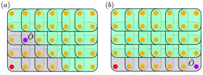
We define P-PEPS with periodic boundary conditions (PBC) as the states generated from the product state through sequential application of unitaries to plaquettes of size () [c.f. Fig. 1(a)]
| (2) |
where and the unitary acts on qudits in the square spanning from to , and we identify the rows and columns . Here the choice of plaquette shape reflects the locality of the unitaries. The ordering of the unitaries fulfils the conditions for . We show an example of in Fig. 1(b), and call the position of the first unitary the source point. To define the state with open boundary conditions (OBC), we simply omit gates that act across boundaries.
P-PEPS is a subclass of PEPS, which are states defined through a network of tensors with one tensor per lattice site [Fig. 1(c)], whose virtual indices are contracted with their neighbors. In two dimensions,
| (3) |
where is a rank-5 tensor on the site that has one physical index of dimension and four virtual indices of bond dimension . The symbol denotes the contraction of all virtual indices. To obtain the PEPS representation of P-PEPS, we decompose the plaquette unitaries into projected entangled-pair operators (PEPO) Cirac et al. (2020) [c.f. Fig. 1(d)]. This allows one to write the whole sequential circuit as a PEPO, which, applied to a product state, yields a PEPS with bond dimension Note (1).
We are particularly interested in cases where each unitary overlaps with at least one of the earlier ones, such that they create correlations. The state shown in Fig. 1(a) is such an example. Sequential circuits with overlapping unitaries efficiently establish correlations between arbitrary locations of the lattice with unitaries Note (1). This should be contrasted with brickwall circuits Gopalakrishnan and Lamacraft (2019) that take unitaries to do so Note (1). This implies that P-PEPS offers a more efficient parametrization of states with correlations across the entire system. Moreover, while P-PEPS have area-law entanglement, brickwall circuits that create long-range correlations will instead lead to states with volume-law entanglement Nahum et al. (2017, 2018); Von Keyserlingk et al. (2018).
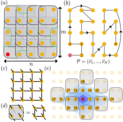
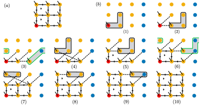
Radial plaquette PEPS (RP-PEPS).— Naively, it takes a circuit depth to create a P-PEPS [c.f. Eq. 2]. However, some orderings allow unitaries to be applied in parallel. A simple example is to arrange the unitaries as a brickwall circuit of depth . Here we define a subclass of P-PEPS, RP-PEPS, where starting from the source point, the positions of the unitaries are ordered such that they can be grouped to multiple layers of commuting unitaries, and each layer act on the boundary of the existing gate-acted region. An example with is illustrated in Fig. 1(e), where the gates are grouped as (denoted by shades of different colors). To resolve ambiguities in the plaquette order, we choose preferred directions in which the position of the plaquette moves. In Fig. 1(e) we choose ‘horizontal first, and positive direction first’. The circuit depth of preparing RP-PEPS is asymptotically , following the scaling in Eq. 1. Moreover, RP-PEPS allow efficient computation of expectation values of local observables that are geometrically close to the source point or the line that passes through the source point along the preferred direction, and this generically implies that correlation functions in these regions decay exponentially. This is reminiscent of isoTNS Zaletel and Pollmann (2020).
The above definitions straightforwardly generalize to higher dimensional lattices, where plaquettes become high-dimensional cubes Note (1). While the general circuit depth for P-PEPS again scales with , RP-PEPS obeys Eq. 1.
Relation to other families of PEPS.—By definition, P-PEPS can be efficiently prepared, have a PEPS description, and host long-range correlations. Now we show that P-PEPS naturally encompass other families of PEPS that are prepared sequentially (SGS and F-PEPS), as well as isoTNS (we follow the definition in Ref. Zaletel and Pollmann (2020), and see Ref. Haghshenas et al. (2019) for a different definition).
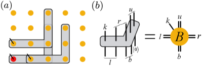
SGS [c.f. Fig. 2(a)] are defined in terms of linear sequential circuits comprising unitaries of length acting on rows across qudits whose columns have been prepared in MPS Bañuls et al. (2008)
| (4) |
The MPS in each column can be put in canonical form, such that they can be written as linear sequential circuits Schön et al. (2005); Bañuls et al. (2008). This allows us to identify the tensor of the corresponding PEPS as two overlapping -qudit unitaries [c.f. Fig. 2(b)]. These two unitaries are contained in a plaquette unitary. Thus, each SGS can be written as an RP-PEPS, with the source point at the bottom left of the lattice in the case of Fig. 2(a).
To be precise, let us denote the class of SGS (P-PEPS) on an lattice with circuit length (plaquette length) as (), we have
| (5) |
The tensors of SGS in the bulk satisfy an isometry condition shown in Fig. 2(d), which is the same condition as is obeyed by the tensors in isoTNS Zaletel and Pollmann (2020). Indeed, as we show in the following, these classes are closely related.
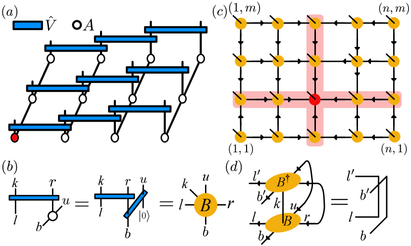
IsoTNS are PEPS [Eq. 3] in which all tensors satisfy isometry conditions that depend on their position in the lattice. Specifically, when all incoming indices of a tensor (denoted by incoming arrows in Fig. 2c) and the physical index are contracted with corresponding indices of the complex conjugate of that tensor, the remaining indices yield the identity. For example, the tensor in the dashed box in Fig. 2(c) obeys [c.f. Fig. 2(d)]
| (6) |
The red shaded lines in Fig. 2(c) are called orthogonality hypersurfaces, which only have incoming arrows, and their intersection is the orthogonality center (OC) Zaletel and Pollmann (2020).
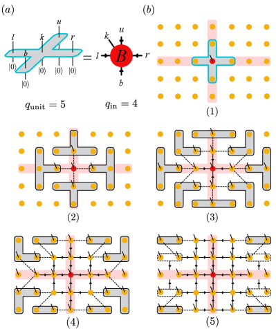
One can prepare isoTNS as RP-PEPS, but restricting the unitaries in the bulk to be ‘L’-shaped, as shown in Fig. 3(a1-6). The required three-qudit unitaries can be written as
| (7) |
where , and the tensor automatically satisfies the isometry condition Eq. 6. Thus each unitary creates an isoTNS site [c.f. Fig. 3(b)].
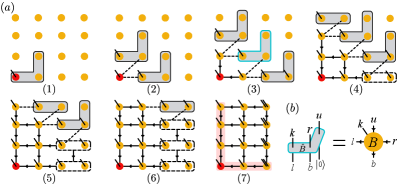
Sequentially applying the gates shown in Fig. 3(a1-6) gives rise to the tensor contraction pattern shown in Fig. 3(a7), which represents an arbitrary isoTNS with OC in the corner. The generated isoTNS has bond dimension and physical dimension , except at the right boundary, where two sites of each row are combined to form a site with physical dimension . Note that arbitrary isoTNS of that geometry with a uniform physical dimension can be embedded in that state by setting the rightmost qudits to zero and treating them as ancillas. Moreover, it is clear from Fig. 3(a) that the circuit depth for preparing isoTNS is . We show in the SI Note (1) that: i) by extending the indices of ‘L’-shaped unitaries to qudits with and changing the source point of the RP-PEPS, isoTNS with arbitrary bond dimension and with OC in the bulk can be prepared. ii) This protocol can be generalized to prepare isoTNS of higher dimensions. Therefore, isoTNS on arbitrary lattices (of size ) admit exact representations as sequential quantum circuits, with the circuit depth scaling as
| (8) |
The above observation shows that isoTNS RP-PEPS. A similar relation also holds between P-PEPS and F-PEPS Pichler et al. (2017), here understood as a generalization to qudits and with arbitrary photon feedback. F-PEPS can be viewed as isoTNS on a lattice with different connectivity Pichler et al. (2017). If we denote () as the class of isoTNS (F-PEPS) on a lattice with bond dimension and physical dimension , we prove in the SI Note (1) that isoTNS (F-PEPS) is contained in RP-PEPS (P-PEPS) with a slightly larger lattice
| (9) |
| (10) |
Having established that both SGS and isoTNS are RP-PEPS with ‘L’-shaped unitaries, we note that SGS has a further condition on the unitaries, namely that they can be decomposed into two unitaries corresponding to the two arms of the L (see Fig. 2b), which indicates that SGS are a subclass of isoTNS. This has direct consequences for the states. While in SGS, local observables can efficiently be calculated anywhere in the lattice, in isoTNS, this requires shifting the OC, which can only be done approximately. Their precise relation is Note (1)
| (11) |
Finally, we note that, since the isometry of the PEPS tensors derives directly from the unitarity of the preparation circuit, we further show that RP-PEPS can be expressed as isoTNS on lattices with unusual connectivities Note (1).
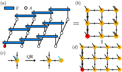
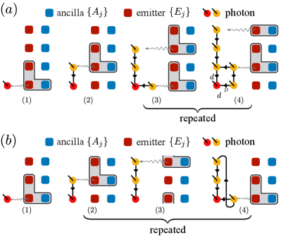
Generating RP-PEPS of flying qub(d)its.— Ref. Schön et al. (2005) introduces a protocol to prepare arbitrary photonic MPS of bond dimension and physical dimension using a photon source comprising a -level ancilla and a -level emitter . The MPS is prepared by repeatedly applying a unitary on the joint ancilla-emitter system, followed by swapping the emitter state into a flying photon, defined in terms of the photon emission isometry
| (12) |
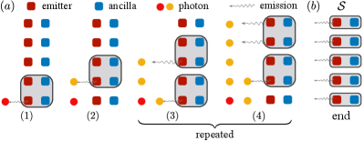
Now we extend the above protocol by considering an array of sequential photon sources coupled to each other as shown in Fig. 4, and show that photonic RP-PEPS can be prepared with this setup.
The protocol is shown in Fig. 4. Here we assume each ancilla has a dimension , so it can be thought of as qudits. Starting with the ancillas and emitters in their ground state , in the step to prepare the -th site of the RP-PEPS, first we apply a unitary that acts on the ancillas and emitters [see Fig. 4(a) for case]. After the unitary, we trigger the photon emission from the emitter (denoted as [cf. Eq. 12]). To disentangle the ancilla from the photons, in the last steps of the protocol, we sequentially swap the effective qudits contained in the ancilla into photons (c.f. Fig. 4b), an operation collectively denoted by . The final state of the system is , with the photonic state
| (13) |
is an arbitrary RP-PEPS with OBC and plaquette size , with its source point at the first photonic qudit. The circuit depth is the same as that of matter-based lattice case [c.f. Eq. 1]. The same protocol also allows to prepare isoTNS Note (1), and this setup can be used to prepare photonic F-PEPS with circuit depth Note (1).
Notice that, at the boundary of the photon source array, the photon emission process emits multiple photons, as visualized in Fig. 4(a4). In contrast to the protocol that produces RP-PEPS on a matter-based lattice, here the overlapping of gates along the horizontal direction are produced by acting on the ancillas. In Ref. Wei et al. (2021b) we propose a cavity-transmon setup to realize of this protocol, and elaborate on how to create the two-dimensional photonic cluster state and the toric code state 222Note that for the cluster state generation, there are specific schemes Lindner and Rudolph (2009); Economou et al. (2010) that do not need ancillas and SWAP gates. These schemes thus require less resources than the present scheme..
Conclusion.—We have introduced P-PEPS and its subclass RP-PEPS, which constitute a natural generalization of sequential preparation protocols from one to higher dimensions. These states satisfy area-law entanglement by construction, combine the capacity to host long-range correlations, topologically ordered states, and a large subclass of PEPS with a simple and efficient preparation protocol. Our work helps to clarify the relation between various relevant classes of PEPS, including SGS Bañuls et al. (2008), F-PEPS Pichler et al. (2017) and isoTNS Zaletel and Pollmann (2020), that we show SGS isoTNS RP-PEPS, and F-PEPS P-PEPS.
The family of states we introduce come with explicit protocols that prepare them in matter-based and photon-based lattices, which makes them promising targets for near-term experimental realization. Furthermore, one can include several layers of sequential plaquettes to increase the expressivity of the ansatz.
We acknowledge funding from ERC Advanced Grant QUENOCOBA under the EU Horizon 2020 program (Grant Agreement No. 742102), and within the D-A-CH Lead-Agency Agreement through project No. 414325145 (BEYOND C), and the European Union’s Horizon 2020 research and innovation program under Grant No. 899354 (FET Open SuperQuLAN).
Supplementary Materials
Appendix A Properties of P-PEPS
A.1 Bond dimension of the PEPS representation of P-PEPS
As discussed in the main text, one can obtain the PEPS representation of P-PEPS by decomposing the plaquette unitaries into projected entangled-pair operators (PEPO) Cirac et al. (2020) (shown in Fig. 1d in the main text). To be precise, given a plaquette unitary of side length , the resulting bond dimension of each PEPO is trivially bounded by , which come from the MPO decomposition of given unitary acting on qudits. Moreover, there are plaquette unitaries acting on each single site. Thus the bond dimension of the PEPS representation of P-PEPS is bounded from above by .
A.2 Efficient computation of certain expectation values
Let us assume we have a local operator . Then its expectation value in a given P-PEPS is
| (14) |
Depending on the ordering of the and the location of in the lattice, it is possible to directly cancel some gates in Eq. 14 with their hermitian conjugate.
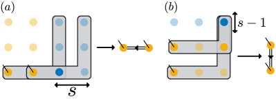
We illustrate this effect in Fig. 5 using a RP-PEPS with the source point in a corner of the lattice. For RP-PEPS, the ordering reflects the distance of the unitary to the source point. In this case, the expectation values of local operators that are geometrically close to the source point can be computed efficiently [c.f. Fig. 5(a)]. Moreover, due to the choice of the preferred direction for plaquettes at equal distance, one finds that also along the line starting from the source point and along the preferred direction, expectation values can be computed efficiently [c.f. Fig. 5(b)].
Note that this is very similar to what happens in isometric tensor networks, in which expectation values of operators close to the OC or the orthogonal hypersurfaces can be calculated efficiently Zaletel and Pollmann (2020).
A.3 Long-range correlation in the P-PEPS, and comparison to brickwall circuits
In case that the plaquette unitaries for creating P-PEPS [Eq. (2) in the main text] overlap with earlier ones, the resulting P-PEPS generally have long-range correlations among arbitrary locations in the lattice. To illustrate this, first let us compare such one-dimensional P-PEPS and the brickwall circuit Gopalakrishnan and Lamacraft (2019), shown in Fig. 6. Here the ‘plaquette’ gates for one-dimensional P-PEPS are local gates of qub(d)its.
In this section, we assume the shape of unitaries in the brickwall circuits is the same as in the case of P-PEPS. A similar discussion between these two circuit structures can be found in Ref. Lin et al. (2021).
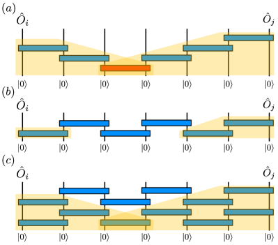
Given a state prepared by quantum circuits, the correlations between two locations are non-zero if the reversed ‘light cones’ starting from these two locations overlap. This is illustrated in one dimension in Fig. 6(a). If we take the same number of unitaries and arrange them in a brickwall circuit (this also belong to P-PEPS), it will be a finite-depth circuit of depth [shown in Fig. 6(b) for ], which only creates correlations up to a distance . To create long-range correlations in brickwall circuits requires a circuit depth of at least [c.f. Fig. 6(c)], which uses many more gates.
The above observation also holds for higher dimensional P-PEPS. Thus, when the plaquette unitaries in Eq. (2) in the main text have overlap with earlier ones, the reversed light cones of two arbitrary locations in the lattice always overlap, at the very least on the first plaquette. For a lattice, it generally take a brickwall circuit of depth to produce long-range correlations among the whole lattice, thus takes gates, many more than for P-PEPS preparation.
Thus P-PEPS contain states with long-range correlation among arbitrary locations in the lattice. Moreover, such long-range correlated states in the form of RP-PEPS can be prepared particularly efficiently, with circuit depth scale as the maximum edge length of the lattice [Eq. (1) in the main text].
Appendix B Preparing arbitrary 2D isoTNS on lattices of stationary qub(d)its
In this section, we show how to extend the circuit pattern in Fig. 3(a) in the main text to prepare arbitrary 2D isoTNS in a square lattice.
B.1 Increase the isoTNS bond dimension
One can increase the bond dimension of isoTNS prepared by sequential circuit in Fig. 3(a) in the main text by making the gates acting on more common sites. In particular, the gate that generate isoTNS of bond dimension acts on the site where . The example of is shown in Fig. 7(a), with the identification of the PEPS bonds shown in Fig. 7(b).
Notice that, unlike the case of RP-PEPS [Eq. (1) in the main text], increasing the indices of the ‘L’-shape unitaries does not change the circuit depth Eq. (8) in the main text of preparing isoTNS, since it is clear from Fig. 7(a) that we can always parallelize the two unitaries on the upper and right side of a given ‘L’-shape unitary.
B.2 Preparing isoTNS with OC at arbitrary location
The protocol in Fig. 3(a) in the main text prepares arbitrary isoTNS of the geometry shown in step 7 of Fig. 3(a) in the main text, where the OC is at the corner of the lattice, marked with the red dot. In general, the number of incoming virtual bonds in an isoTNS tensor is directly related to the number of outgoing indices for the unitary, as
| (15) |
For example, the isoTNS tensor shown in Fig. 3(b) in the main text are created with three-qudit unitaries (), since there are two incoming indices () for that tensors. When OC at an arbitrary location inside the bulk (like that in Fig. 2a in the main text), the tensor at OC has incoming virtual bonds, thus one need a 5-qudit unitary to prepare it, which is shown in Fig. 8(a). Thus we can use the circuit pattern in Fig. 8(b) to prepare isoTNS with OC in the bulk of the lattice. In step 1, we prepare the tensor at OC by applying a 5-qudit unitary. Then the tensors at the orthogonality hypersurface are prepared by 4-qudit unitaries, for example, shown in step 2. Then one can apply the same procedure as that in Fig. 3(a) in the main text to grow the size of the prepared isoTNS on four regions separated by the orthogonality hypersurface, and use the sites on both left and right boundaries of the lattice as ancillas, to create an arbitrary isoTNS of bond dimension and physical dimension , with OC at an arbitrary location of the lattice. The method to increase the bond dimensions also naturally applies in this scenario.
Preparing isoTNS with OC inside the bulk of the lattice not only makes the class of isoTNS with open boundary conditions we prepare complete but also has practical relevance for the state preparation speed. As the region of prepared sites expands along all directions simultaneously, one can prepare an isoTNS with OC at the center four times faster than one with the OC at the corner. We also point out that the isoTNS with OC inside the bulk is also naturally contained in the class of P-PEPS, as we can just cover the local gates shown in Fig. 8(b) inside appropriate plaquettes and the ordering of plaquette gates naturally captures the sequential ordering in Fig. 8(b).
B.3 Ancilla in preparing isoTNS with uniform bond dimensions
As shown in the main text Fig. 3(a) and the previous sections [c.f. Fig. 8(b) and Fig. 13(b)], one need to use some ancillas when preparing isoTNS. This comes from the mechanism of connecting the tensors of the isoTNS, that we need to let the neighboring gates have overlapping regions to create virtual bonds of the tensors. As a result, when reaching the boundary of the system, we have to merge sites to obtain a general isoTNS of that geometry, for example as shown in Fig. 3(a6-7) in the main text. Without merging, the resulting state would lack vertical bonds between the rightmost sites. Clearly one can embed arbitrary isoTNS of uniform bond dimension and smaller lattice into that geometry, treating the sites on the boundary as ancillas.
We show the usage of ancilla more explicitly on the right and upper boundary of the lattice in Fig. 9. For ‘L’-shape gates of the direction shown there, we need additional columns and rows of qudits as ancilla, where for creating isoTNS of bond dimension . Thus overall, given such an isoTNS with OC in the bulk of size , we will need a lattice, where the sites on the boundary of the lattice act as ancillas.
Moreover, one also needs to use ancilla when creating photonic isoTNS with uniform bond dimensions. We will elaborate it in the photonic isoTNS generation protocol around Fig. 14.
Appendix C Proof of isoTNS RP-PEPS [Eq. (9) in the main text]
It is clear from the previous section that, to produce isoTNS of bond dimension in a lattice, one needs a sequential quantum circuit that acts on a lattice [c.f. Fig. 9], where the sites on the boundary are used as ancillas. Also notice that in Fig. 9(b) the length of the vertical arm of the ‘L’-shape unitary at the upper boundary of the lattice is also slightly reduced. Thus we need to formally put an additional row of ancillas in Fig. 9(b) to make that ‘L’-shape unitary properly covered in a plaquette unitary.
Overall, We can cover the isoTNS preparation circuit into the RP-PEPS preparation circuit on a lattice, where the largest plaquette size is determined by the gate that prepares the OC of isoTNS [c.f. Fig. 8(a)], where we need a plaquette of side length . This thus proves the relation between isoTNS and RP-PEPS [Eq. (9) in the main text]:
A similar argument also holds in higher dimensions, that arbitrary isoTNS is contained in RP-PEPS of slightly bigger lattices.
At last, we point out that, if we are allowed to move the location of the ancilla, we could reduce the number of ancillas to the order of by efficiently reuse the ancilla that has been disentangled after providing the virtual bonds. For example, in Fig. 3(a) in the main text there are always only two ancillas that are under operation or being entangled to the system during the state preparation procedure.
Appendix D Representing RP-PEPS as isoTNS
The sequential application of local quantum gates that have overlapping sites naturally defines a ‘causal’ structure, and the unitarity of gates implies certain isometry conditions. One can view each unitary as a tensor (see Fig. 10(a)), with its incoming and outgoing indices that have overlap with other unitaries as the virtual bonds, and the outgoing indices that do not further connect to other gates as the physical bond. In this way, we can write an arbitrary RP-PEPS as isoTNS. The simplest example of RP-PEPS is shown in Fig. 10(b). Compare to standard isoTNS Zaletel and Pollmann (2020) [c.f. Fig. 2(a) in the main text], the isoTNS representation of RP-PEPS has unusual connectivity and spatial non-uniform bond dimensions and physical dimensions. By further increasing and changing the ordering , the isoTNS representation of RP-PEPS will contain virtual bonds that connect more distant sites and more unusual connectivity.

Appendix E Preparing higher-dimensional P-PEPS and isoTNS
It is desirable to generalize our protocols to prepare higher-dimensional P-PEPS and isoTNS, since these states potentially efficiently characterize the ground state of higher-dimensional local Hamiltonians Tepaske and Luitz (2021), with prominent examples like the three-dimensional cluster state Raussendorf et al. (2006); Russo et al. (2019).
Here we briefly discuss how to generalize our scheme to higher dimensions. First, the P-PEPS can naturally be extended to higher dimensions by sequentially applying higher-dimensional cubes of side length . For a -dimensional lattice of size , the P-PEPS is still of form [Eq. (2) in the main text]:
where now the position vector . Other quantities like the ordering and the state with open boundary conditions are defined in the same way as two-dimensional case, and it is clear that the worst-case circuit depth is of .
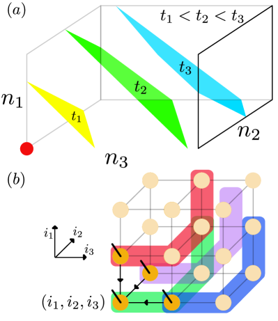
The RP-PEPS can also be defined in the same way, as starting from the source point, we group the unitaries into layers, and each layer of the gates acts on -cubes across the boundary of the gate-acted region, which ballistically expand this region. The three-dimensional case is illustrated in Fig. 11(a). We also need to define the preferred direction as a permutation of directions . If we assume the preferred directions is , i.e. the first index of the position vector grows first, we will get the following depth:
which lead to the scaling Eq. (1) in the main text.
Compare to P-PEPS, it is less obvious to obtain the exact circuit representation of isoTNS in higher dimension. Let us first draw some intuition of this representation from our two-dimension case. In the main text, the isoTNS with the geometry shown in Fig. 3(a7) in the main text have its bulk tensor equivalent to a three-qudit gate acting on the sites , and . Notice that the geometry of is not symmetric for the index , which reflect the fact that is the preferred direction of the underlying RP-PEPS in Fig. 3(a).
It turns out that the tensor of -dimensional isoTNS with bond dimension can be mapped to a unitary that acts on qudits, such that the number of the tensor indices will match the number of incoming and outgoing indices of the unitary with one index acts on the reference state , which is also . For example, in the two-dimensional case [Fig. 3(b) in the main text], the PEPS tensor have 5 indices, corresponds to a 3-qudit unitary with a single input index as reference state .
If we follow the same sequential ordering for the RP-PEPS discussed in this section, the unitary that creates a single isoTNS tensor acts on the sites
For example, to create three-dimensional isoTNS, we apply four-qudit unitary that acts on
| (16) |
Several adjacent unitaries for preparing isoTNS of bond dimension are shown in Fig. 11(b) with different colors. The geometric overlapping of these unitaries gives rise to an isoTNS in a regular three-dimensional lattice, and it is clear that isoTNS RP-PEPS also holds in higher dimensions. Fig. 11(b) also shows that, given a unitary , its adjacent unitaries commute with each other and can be implemented in the same layer of circuit. This eventually lead to a circuit depth for preparing -dimensional isoTNS on a lattice as [c.f. Eq. (8) in the main text]
which is slightly smaller than that for preparing RP-PEPS by a factor of .
At last, one can also generalize the photon generation protocol to higher dimensions in the same way. To prepare a -dimensional photonic lattice, we need a -dimensional array where each site consists of an -level ancilla and an -level emitter as shown in Fig. 4 in the main text. Together the photon emission of emitters, one can operate the same sequential generation protocol as shown in Fig. 4 in the main text, where we replace the unitaries by () to prepare -dimensional RP-PEPS (isoTNS).
Appendix F Proof of SGS isoTNS [c.f. Eq. (11) in the main text]
As already discussed in the main text, the SGS admit a PEPS representation Bañuls et al. (2008). In this section, we prove SGS is a strict subclass of isoTNS using graphical notations. As introduced in the main text, the SGS is prepared by coupling unitaries on multiple lines of MPS. Without loss of generality, we can assume the MPS are all in the canonical form, with their orthogonality centers at the bottom of the lattice, as we show in Fig. 12(a).
In SGS, the unitaries in the bulk couple neighboring columns. The PEPS tensor inside the bulk of the lattice takes the form Bañuls et al. (2008)
| (17) |
Notice this relation is the same as that in Fig. 2(b) in the main text, and we further use the arrows to denote the isometry conditions. Depending on the bond dimension of the underlying MPS and the number of qub(d)its that the unitaries acts on, the PEPS representation of SGS could have different bond dimensions in the horizontal and vertical bonds. Without loss of generality, we assume a uniform bond dimension in the bulk. Also notice that, at the left boundary of the two-dimensional lattice (the case of is shown in Fig. 12a), the corresponding PEPS sites (denoted by the dashed box) have higher vertical bond dimension as , and on the right boundary we group sites in each row (shown in the rightmost dashed box) as one, as PEPS sites with bond dimension and physical dimension .
Thus SGS in Fig. 12(a) can be mapped to PEPS of bond dimension and physical dimension , as shown in Fig. 12(b) for the case of . In Fig. 12(b) we further use the isoTNS notations, as in the following we will show that the PEPS representation of arbitrary SGS is an isoTNS. We also point out that, one can do QR decomposition on the tensors that have multiple physical indices, to separate them to multiple tensor sites that have physical dimension and also satisfy isometry conditions (shown in Fig. 12c). In this way, the isoTNS in Fig. 12(b) can always be written as an isoTNS of a uniform bond dimension that have the same lattice size as the original SGS (Fig. 12d).
Proposition 1
The PEPS representation of SGS [c.f. Fig. 12(b)] is an isoTNS.
Proof: One can directly check the isometry condition of the corresponding tensors in Fig. 12(b). For the sites in the bulk, the unitarity of and the canonical form of lead to
| (18) |
where the connected lines denotes the contraction of the corresponding indices. This directly leads to the isometry condition of SGS tensor in the bulk [Eq. 17]:
| (19) |
Analogously, one can check all tensors in the boundaries also satisfy the corresponding isometry conditions, with arrow directions denoted in Fig. 12(b). Thus the PEPS representation of SGS is itself an isoTNS (c.f. Fig. 12).
From the reverse direction, isoTNS is not necessarily a SGS. In the main text, we have qualitatively shown that the circuit representation of a tensor for SGS and isoTNS are quite similar, as they both acts on the same set of the qudits. In the case of bond dimension , for SGS it contain two two-qudit unitaries [c.f. Fig. 2(d) in the main text], while in the case of isoTNS the circuit is a generic three-qudit unitary [c.f. Fig. 3(b) in the main text].
Proposition 2
A single PEPS tensor corresponding to a SGS site [c.f. Eq. (17)] does not cover arbitrary isoTNS tensor [c.f. Fig. 3(b) in the main text] with the same isometry condition.
Proof: Let us consider the single PEPS tensor that have the same structure as that come from the SGS [c.f. Eq. 17]. For simplicity, we consider the case, where has both physical dimension and bond dimension , with the isometry condition shown by below Eq. 20. One can apply a QR decomposition to the tensor, getting
| (20) |
where the part is an isometry (due to the QR decomposition), and each black line denote a bond of dimension . Thus, an arbitrary isoTNS tensor satisfying isometry condition is equivalently represented by arbitrary and that satisfy
| (21) |
It is clear that coming from an isoTNS, the resulting tensor coming from QR decomposition [Eq. 21] does not necessarily satisfy the condition for SGS Eq. 18. They differ in the following points: i) For the part of SGS, one requires a full identity on the indices and as shown in Eq. 18. However, for the part of isoTNS, we only require an identity relation on when we contract the other three indices . ii) The index that connects two tensors and for isoTNS can generally have dimension , while the one for SGS can only have the dimension . The above point i) is particularly important, since even if one arbitrarily increases the bond dimension of the SGS, one can still find isoTNS that does not have an identity condition on the index , thus makes SGS unable to cover the full class of isoTNS with any non-trivial bond dimension .
Thus SGS is a strict subclass of isoTNS. More precisely, we have [c.f. Eq. (11) in the main text]:
Here we have used the PEPS representation of SGS [c.f. Fig. 12(d)]. We also point out that, here the bond dimension of the isoTNS aims to capture the bond dimension at the boundary of the lattice, however, the majority of the sites in the bulk of the lattice just have , thus isoTNS of ‘almost’ cover the class of SGS of circuit length .
The difference between SGS and isoTNS is reflected in their qualitative difference, that SGS admits efficient computation of local correlators at an arbitrary location of the lattice Bañuls et al. (2008), however, isoTNS can only shift OC approximately Zaletel and Pollmann (2020), thus compute local correlators at an arbitrary location only in an approximate way.
Appendix G Proof of F-PEPS P-PEPS [Eq. (10) in the main text]
The F-PEPS proposed in Ref. Pichler et al. (2017) is a subclass of PEPS produced by photon feedback from a single emitter. It is clear from Ref. Pichler et al. (2017) that, F-PEPS is a PEPS with shifted PBC, where each tensor satisfies an isometry condition. Thus, we can represent F-PEPS as isoTNS with a shifted PBC shown in Fig. 13(a), where the isometry conditions are denoted by the arrows. In this section, we will show the preparation protocol of F-PEPS on lattices of stationary qub(d)its using a sequential circuit, which will naturally serve as proof of the fact that F-PEPS P-PEPS [Eq. (10) in the main text].
The direction of the arrows in the isoTNS representation of F-PEPS [c.f. Fig. 13(a)] indicates a full sequential ordering of its preparation circuit. In particular, the site on the boundary of each row has to be prepared earlier than the site on the boundary of the next row. Thus unlike the preparation of isoTNS with OBC [c.f. Fig. 3(a) in the main text], the preparation of F-PEPS does not allow the gates to be applied simultaneously along different directions.
We can prepare F-PEPS with a full sequential circuit shown in Fig. 13(b). Compare to the isoTNS preparation protocol [c.f. Fig. 3(a) in the main text], here we modify the shape of gates that create sites on the right boundary of each row (denoted with green boxes in steps 3 and 6), such that these gates now also act on the first site of the next row. The coupling of different boundaries creates additional virtual bonds of the resulting isoTNS, thus give us an arbitrary isoTNS of bond dimension of the geometry shown in Fig. 13(b10), with shifted PBC. Here we have used the sites on the right boundary of the lattice as ancillas.
Similar to the isoTNS case [c.f. Fig. 9], to create arbitrary F-PEPS with larger bond dimension , we need to let the neighboring gates to have common sites, thus require columns and rows of ancillas (later we will put rows of ancillas, to ensure the gates are covered by plaquette unitaries). Also, the sequential circuit of the maximal size are those that couples to boundaries of the lattice( shown as green boxes in Fig. 13), and they can be contained in plaquette of side length . With that, it is clear that [c.f. Eq. (10) in the main text]
The above construction shows that F-PEPS P-PEPS, and serve as the way to create them. To create a F-PEPS on lattice, the circuit depth is . We also point out that isoTNS with other kinds of periodic boundary conditions can be prepared in the same way.
Appendix H Preparing isoTNS and F-PEPS of flying qub(d)its
As shown in the main text, each isoTNS tensor can be mapped to a ‘L’-shape unitary [c.f. Eq. (7) in the main text]. Thus using the ancilla-emitter array setup shown in Fig. 4 in the main text, we are able to create photonic isoTNS.
The procedure to produce photonic isoTNS of bond dimension with the open boundary condition is shown in Fig. 14(a). Here we follow the RP-PEPS generation protocol in Fig. 4 in the main text, and the unitary that prepares the -th isoTNS site acts on the ancilla and emitters . Due to the sequential nature of the protocol, the OC sits on the first photonic qudit being produced. One can also increase the bond dimension of the resulting isoTNS in the same way as shown in Fig. 7(a), by increasing the ancilla dimension and increase the length of the ‘L’-shape gate along the emitters. Also, similar to the matter-based isoTNS case [c.f. Fig. 9(b)], we need to put additional qudits (each of the dimension ) with on the top or bottom boundary of the array, which will be used to create virtual bonds of the isoTNS tensors.
In this case, this photonic isoTNS is again contained in the photonic RP-PEPS on a slightly larger lattice.
At last, by another simple modification of the above protocol, our platform can also prepare photonic F-PEPS, which are isoTNS with shifted periodic boundary conditions (sPBC). In Fig. 14(b), we show the steps to prepare F-PEPS. The key point is step (3), which applies a gate that couples two boundaries of the lattice, providing the virtual bond for sPBC shown in step (4). This indicates that the class of states that our ancilla-emitter array setup can prepare is strictly larger than that the non-Markovian feedback approaches can prepare Pichler et al. (2017); Dhand et al. (2018); Xu and Fan (2018); Wan et al. ; Zhan and Sun (2020); Shi and Waks ; Bombin et al. .
Compared to the non-Markovian feedback approaches Pichler et al. (2017); Dhand et al. (2018); Xu and Fan (2018); Wan et al. ; Zhan and Sun (2020); Shi and Waks ; Bombin et al. , our array-based approach does not require interaction with the emitted photons, therefore is easier to implement experimentally. Specifically, it allows one to implement generic unitaries and makes it possible to increase the complexity of the state by acting on more qub(d)its.
References
- Verstraete et al. (2008) F. Verstraete, V. Murg, and J. I. Cirac, Advances in Physics 57, 143 (2008).
- Orús (2019) R. Orús, Nature Reviews Physics 1, 538 (2019).
- Cirac et al. (2020) J. I. Cirac, D. Perez-Garcia, N. Schuch, and F. Verstraete, “Matrix product states and projected entangled pair states: Concepts, symmetries, and theorems,” (2020), arXiv:2011.12127 .
- Fannes et al. (1992) M. Fannes, B. Nachtergaele, and R. F. Werner, Communications in mathematical physics 144, 443 (1992).
- (5) D. Perez-Garcia, F. Verstraete, M. M. Wolf, and J. I. Cirac, arXiv:0608197 [quant-ph] .
- Schollwöck (2011) U. Schollwöck, Annals of Physics 326, 96 (2011).
- Hastings (2007) M. B. Hastings, Journal of Statistical Mechanics: Theory and Experiment 2007, P08024 (2007).
- Verstraete and Cirac (2006) F. Verstraete and J. I. Cirac, Physical Review B 73, 1 (2006).
- (9) F. Verstraete and J. I. Cirac, arXiv:0407066 [cond-mat] .
- Verstraete et al. (2006) F. Verstraete, M. M. Wolf, D. Perez-Garcia, and J. I. Cirac, Physical Review Letters 96, 1 (2006).
- Schuch et al. (2010) N. Schuch, I. Cirac, and D. Pérez-García, Annals of Physics 325, 2153 (2010).
- Levin and Wen (2005) M. A. Levin and X.-G. Wen, Physical Review B 71, 45110 (2005).
- Gu et al. (2009) Z.-C. Gu, M. Levin, B. Swingle, and X.-G. Wen, Physical Review B 79, 85118 (2009).
- Buerschaper et al. (2009) O. Buerschaper, M. Aguado, and G. Vidal, Physical Review B 79, 085119 (2009).
- Degen et al. (2017) C. L. Degen, F. Reinhard, and P. Cappellaro, Reviews of Modern Physics 89, 1 (2017).
- Dür et al. (2000) W. Dür, G. Vidal, and J. I. Cirac, Physical Review A 62, 62314 (2000).
- Greenberger et al. (1989) D. M. Greenberger, M. A. Horne, and A. Zeilinger, in Bell’s theorem, quantum theory and conceptions of the universe (Springer, 1989) pp. 69–72.
- Briegel and Raussendorf (2001) H. J. Briegel and R. Raussendorf, Physical Review Letters 86, 910 (2001).
- Hein et al. (2004) M. Hein, J. Eisert, and H. J. Briegel, Physical Review A 69, 62311 (2004).
- Russo et al. (2019) A. Russo, E. Barnes, and S. E. Economou, New Journal of Physics 21, 55002 (2019).
- Azuma et al. (2015) K. Azuma, K. Tamaki, and H. K. Lo, Nature Communications 6 (2015), 10.1038/ncomms7787.
- Kruszynska and Kraus (2009) C. Kruszynska and B. Kraus, Physical Review A 79, 52304 (2009).
- Rossi et al. (2013) M. Rossi, M. Huber, D. Bruß, and C. Macchiavello, New Journal of Physics 15 (2013), 10.1088/1367-2630/15/11/113022.
- Schön et al. (2005) C. Schön, E. Solano, F. Verstraete, J. I. Cirac, and M. M. Wolf, Physical Review Letters 95, 1 (2005).
- Schön et al. (2007) C. Schön, K. Hammerer, M. M. Wolf, J. I. Cirac, and E. Solano, Physical Review A 75, 1 (2007).
- (26) A. Smith, B. Jobst, A. G. Green, and F. Pollmann, arXiv:1910.05351 .
- Lin et al. (2021) S.-H. Lin, R. Dilip, A. G. Green, A. Smith, and F. Pollmann, PRX Quantum 2, 10342 (2021).
- Gheri et al. (1998) K. M. Gheri, C. Saavedra, P. Törmä, J. I. Cirac, and P. Zoller, Physical Review A 58, R2627 (1998).
- Saavedra et al. (2000) C. Saavedra, K. M. Gheri, P. Törmä, J. I. Cirac, and P. Zoller, Physical Review A 61, 62311 (2000).
- Lindner and Rudolph (2009) N. H. Lindner and T. Rudolph, Physical Review Letters 103, 1 (2009).
- Schwartz et al. (2016) I. Schwartz, D. Cogan, E. R. Schmidgall, Y. Don, L. Gantz, O. Kenneth, N. H. Lindner, and D. Gershoni, Science 354, 434 (2016).
- (32) K. Tiurev, M. H. Appel, P. L. Mirambell, M. B. Lauritzen, A. Tiranov, P. Lodahl, and A. S. Sørensen, arXiv:2007.09295 .
- Eichler et al. (2015) C. Eichler, J. Mlynek, J. Butscher, P. Kurpiers, K. Hammerer, T. J. Osborne, and A. Wallraff, Physical Review X 5, 1 (2015).
- Besse et al. (2020) J.-C. Besse, K. Reuer, M. C. Collodo, A. Wulff, L. Wernli, A. Copetudo, D. Malz, P. Magnard, A. Akin, M. Gabureac, G. J. Norris, J. I. Cirac, A. Wallraff, and C. Eichler, Nature Communications 11, 1 (2020).
- Wei et al. (2021a) Z.-Y. Wei, D. Malz, A. González-Tudela, and J. I. Cirac, Phys. Rev. Research 3, 23021 (2021a).
- (36) S. C. Wein, J. C. Loredo, M. Maffei, P. Hilaire, A. Harouri, N. Somaschi, A. Lemaître, I. Sagnes, L. Lanco, O. Krebs, A. Auffèves, C. Simon, P. Senellart, and C. Antón-Solanas, arXiv:2106.02049 .
- Lamata et al. (2008) L. Lamata, J. León, D. Pérez-García, D. Salgado, and E. Solano, Physical Review Letters 101, 1 (2008).
- Cramer et al. (2010) M. Cramer, M. B. Plenio, S. T. Flammia, R. Somma, D. Gross, S. D. Bartlett, O. Landon-Cardinal, D. Poulin, and Y. K. Liu, Nature Communications 1, 147 (2010).
- Saberi (2011) H. Saberi, Physical Review A 84, 1 (2011).
- Delgado et al. (2007) Y. Delgado, L. Lamata, J. León, D. Salgado, and E. Solano, Physical review letters 98, 150502 (2007).
- Osborne et al. (2010) T. J. Osborne, J. Eisert, and F. Verstraete, Physical Review Letters 105, 1 (2010).
- Huggins et al. (2019) W. Huggins, P. Patil, B. Mitchell, K. Birgitta Whaley, and E. Miles Stoudenmire, Quantum Science and Technology 4 (2019), 10.1088/2058-9565/aaea94.
- (43) M. Foss-Feig, D. Hayes, J. M. Dreiling, C. Figgatt, J. P. Gaebler, S. A. Moses, J. M. Pino, and A. C. Potter, arXiv:2005.03023 .
- Barratt et al. (2021) F. Barratt, J. Dborin, M. Bal, V. Stojevic, F. Pollmann, and A. G. Green, npj Quantum Information 7, 79 (2021).
- Ran (2020) S. J. Ran, Physical Review A 101, 1 (2020).
- Schuch et al. (2007) N. Schuch, M. M. Wolf, F. Verstraete, and J. I. Cirac, Physical Review Letters 98, 1 (2007).
- (47) K. J. Satzinger, Y. Liu, A. Smith, C. Knapp, M. Newman, C. Jones, Z. Chen, C. Quintana, X. Mi, A. Dunsworth, and Others, arXiv:2104.01180 .
- Liu et al. (2021) Y.-J. Liu, K. Shtengel, A. Smith, and F. Pollmann, , 1 (2021), arXiv:2110.02020 .
- Bañuls et al. (2008) M. C. Bañuls, D. Pérez-García, M. M. Wolf, F. Verstraete, and J. I. Cirac, Physical Review A 77, 1 (2008).
- Pichler et al. (2017) H. Pichler, S. Choi, P. Zoller, and M. D. Lukin, Proceedings of the National Academy of Sciences 114, 11362 (2017).
- Zaletel and Pollmann (2020) M. P. Zaletel and F. Pollmann, Physical Review Letters 124, 37201 (2020).
- Soejima et al. (2020) T. Soejima, K. Siva, N. Bultinck, S. Chatterjee, F. Pollmann, and M. P. Zaletel, Physical Review B 101, 1 (2020).
- Economou et al. (2010) S. E. Economou, N. Lindner, and T. Rudolph, Physical Review Letters 105, 1 (2010).
- Gimeno-Segovia et al. (2019) M. Gimeno-Segovia, T. Rudolph, and S. E. Economou, Physical Review Letters 123, 70501 (2019).
- Bekenstein et al. (2020) R. Bekenstein, I. Pikovski, H. Pichler, E. Shahmoon, S. F. Yelin, and M. D. Lukin, Nature Physics 16, 676 (2020).
- Dhand et al. (2018) I. Dhand, M. Engelkemeier, L. Sansoni, S. Barkhofen, C. Silberhorn, and M. B. Plenio, Physical Review Letters 120 (2018).
- Xu and Fan (2018) S. Xu and S. Fan, APL Photonics 3 (2018), 10.1063/1.5044248.
- (58) K. Wan, S. Choi, I. H. Kim, N. Shutty, and P. Hayden, “Fault-tolerant qubit from a constant number of components,” arXiv:2011.08213 .
- Zhan and Sun (2020) Y. Zhan and S. Sun, Physical Review Letters 125, 223601 (2020).
- (60) Y. Shi and E. Waks, arXiv:2101.07772 .
- (61) S. Bartolucci, P. Birchall, H. Bombin, H. Cable, C. Dawson, M. Gimeno-Segovia, E. Johnston, K. Kieling, N. Nickerson, M. Pant, F. Pastawski, T. Rudolph, and C. Sparrow, arXiv:2101.09310 .
- (62) H. Bombin, I. H. Kim, D. Litinski, N. Nickerson, M. Pant, F. Pastawski, S. Roberts, and T. Rudolph, arXiv:2103.08612 .
- Blais et al. (2021) A. Blais, A. L. Grimsmo, S. M. Girvin, and A. Wallraff, Reviews of Modern Physics 93, 25005 (2021).
- Bruzewicz et al. (2019) C. D. Bruzewicz, J. Chiaverini, R. McConnell, and J. M. Sage, Applied Physics Reviews 6 (2019), 10.1063/1.5088164, arXiv:1904.04178 .
- Saffman (2016) M. Saffman, Journal of Physics B: Atomic, Molecular and Optical Physics 49, 202001 (2016).
- Note (1) See Supplemental Material for more details, which includes Refs.[74,75].
- Gopalakrishnan and Lamacraft (2019) S. Gopalakrishnan and A. Lamacraft, Physical Review B 100, 1 (2019).
- Nahum et al. (2017) A. Nahum, J. Ruhman, S. Vijay, and J. Haah, Physical Review X 7, 1 (2017).
- Nahum et al. (2018) A. Nahum, S. Vijay, and J. Haah, Physical Review X 8, 21014 (2018).
- Von Keyserlingk et al. (2018) C. W. Von Keyserlingk, T. Rakovszky, F. Pollmann, and S. L. Sondhi, Physical Review X 8, 21013 (2018).
- Haghshenas et al. (2019) R. Haghshenas, M. J. O’Rourke, and G. K. L. Chan, Physical Review B 100, 1 (2019).
- Wei et al. (2021b) Z.-Y. Wei, J. I. Cirac, and D. Malz, arXiv preprint arXiv:2109.06781 (2021b).
- Note (2) Note that for the cluster state generation, there are specific schemes Lindner and Rudolph (2009); Economou et al. (2010) that do not need ancillas and SWAP gates. These schemes thus require less resources than the present scheme.
- Tepaske and Luitz (2021) M. S. J. Tepaske and D. J. Luitz, Phys. Rev. Research 3, 23236 (2021).
- Raussendorf et al. (2006) R. Raussendorf, J. Harrington, and K. Goyal, Annals of Physics 321, 2242 (2006).