Sequential Fair Resource Allocation under a Markov Decision Process Framework
Abstract
We study the sequential decision-making problem of allocating a divisible resource to agents that reveal their stochastic demands on arrival over a finite horizon. Our goal is to design fair allocation algorithms that exhaust the available resource budget. This is challenging in sequential settings where information on future demands is not available at the time of decision-making. We formulate the problem as a discrete time Markov decision process (MDP). We propose a new algorithm, SAFFE, that makes fair allocations with respect to all demands revealed over the horizon by accounting for expected future demands at each arrival time. Using the MDP formulation, we show that the allocation made by SAFFE optimizes an upper bound of the Nash Social Welfare fairness objective. We further introduce SAFFE-D, which improves SAFFE by more carefully balancing the trade-off between the current revealed demands and the future potential demands based on the uncertainty in agents’ future demands. We bound its gap to optimality using concentration bounds on total future demands. On synthetic and real data, we compare SAFFE-D against a set of baseline approaches, and show that it leads to more fair and efficient allocations and achieves close-to-optimal performance.
1 Introduction
The problem of multi-agent resource allocation arises in numerous disciplines including economics Cohen et al. (1965), power system optimization Yi et al. (2016); Nair et al. (2018), and cloud computing Balasubramanian et al. (2007); Abid et al. (2020). It comes in various flavors depending on the nature of resources, the agents’ behavior, the timing of allocation decisions, and the overall objective of the allocation process. A common element shared by various settings is the existence of a limited resource that needs to be distributed to various agents based on their reported requests.
There are various objectives that one might wish to optimize in the context of resource allocation. While the goal may be to maximize efficiency (e.g, minimize the leftover resource), other objectives combine efficiency with various notions of fairness. Among different fairness metrics, Nash Social Welfare (NSW) is a well-known objective defined as the geometric mean of the agents’ “satisfaction” with their allocation Nash (1950); Kaneko and Nakamura (1979). In the offline setting where we observe all requests prior to making an allocation decision, the NSW solution enjoys favorable properties including being Pareto-efficient (for any other allocation there would be at least one agent who is worse off compared to the current one), envy-free (no agent prefers any other agent’s allocation), and proportionally fair (every agent gets their fair share of the resource) Varian (1973), and thus exhausts the total budget under a limited resource.
In this work, we consider the much more challenging online (or sequential) setting where agents place requests in a sequential manner, and allocation decisions have to be made instantaneously and are irrevocable. In order to achieve fairness we need to reserve the resource for anticipated future demands, which can lead to wasted resources if the expected future agents do not arrive. Unlike previous work on sequential allocation Lien et al. (2014); Sinclair et al. (2022), we consider a more general setup where agents can arrive several times over the horizon, and their demand size is not restricted to a finite set of values. This setting has important applications such as allocating stock inventory on a trading platform or supplier-reseller settings (e.g., automaker-dealer) where the degree of fairness impacts their relationship Kumar et al. (1995); Yilmaz et al. (2004).
Contributions
We consider a general sequential setting where truthful agents can submit multiple demands for divisible resources over a fixed horizon, and the goal is to ensure fairness over this horizon. There is no standard notion of fairness in the sequential setting, as it may be impossible to satisfy all of the favorable fair properties simultaneously Sinclair et al. (2022). Therefore, online allocation algorithms are commonly evaluated in comparison to their offline (or hindsight) counterpart Gallego et al. (2015); Sinclair et al. (2022). We formulate the sequential problem in terms of maximizing expected NSW in hindsight, and design algorithms that explicitly optimize for this.
The multiple-arrival setting requires being mindful of all past and future requests when responding to an agent’s current demand. We propose a new algorithm SAFFE-D, which determines fair allocations by accounting for all expected future unobserved demands (e.g., based on historical information on agent demands) as well as each agent’s past allocations. In addition, we introduce a tunable discounting term in SAFFE-D, which improves both efficiency and fairness. It uses the uncertainty of future demands to balance the contention between allocating the resource now vs reserving it for the future across the entire horizon. We provide theoretical upper bounds on the sub-optimality gap of SAFFE-D using concentration bounds around the expected future demands, which also guide us in tuning the discounting term of SAFFE-D. Finally, we use numerical simulations and real data to illustrate the close-to-optimal performance of SAFFE-D in different settings, and we compare it against existing approaches and a reinforcement learning policy.
2 Problem Formulation
We consider a supplier that has a divisible resource with a limited budget size , and truthful agents that arrive sequentially over time steps requesting (possibly fractional) units of the resource. At time , agent arrives and reveals its demand sampled from distribution . We assume that each agent has at least one demand over the horizon . The supplier observes demands , and makes an allocation , where denotes the resource amount allocated to agent . We assume that the allocations are immediately taken by the agents and removed from the inventory. We also assume that the setting is repeated, i.e., after time steps, a new budget is drawn and the next allocation round of time steps starts.
Agent has a utility function , representing its satisfaction with the allocation given its (latent) demands. The utility function is a non-decreasing non-negative concave function. In this work, we consider the following utility function, where an agent’s utility linearly increases with its total allocation up to its total request
| (1) |
An agent with the utility function in (1) only values an allocation in the time step it requests the resource, and not in earlier or later steps, which is suitable in settings where the allocation process is time sensitive and the supplier is not able to delay the decision-making outside of the current time step. If all agent demands are known to the supplier at the time of decision-making, they can be used for determining the allocations. This setting is often referred to as offline. However, in the online or sequential setting, the agent demands are gradually revealed over time, such that the supplier only learns about at time . We present the paper in terms of a single resource; however, the setting extends to multiple resources as described in Appendix A.
Notation
. For vectors and , we use to denote for each . denotes a zero vector. denotes the Normal distribution with mean and variance .
2.1 Fairness in Allocation Problems
The supplier aims to allocate the resource efficiently, i.e., with minimal leftover at the end of horizon , and in a fair manner maximizing NSW. The NSW objective is defined as , where reflects the weight assigned to agent by the supplier. NSW is a balanced compromise between the utilitarian welfare objective, which maximizes the utility of a larger number of agents, and the egalitarian welfare objective, which maximizes the utility of the worst-off agent. Since
the logarithm of NSW is often used as the objective function in allocation problems, such as in the Eisenberg-Gale program Eisenberg and Gale (1959). We refer to this as the log-NSW objective.
In the sequential setting, it is not guaranteed that there always exists an allocation that is simultaneously Pareto-efficient, envy-free, and proportional (Sinclair et al., 2020, Lemma 2.3). Motivated by the properties of the NSW objective in the offline setting, and the fact that our repeated setting can be viewed as multiple draws of the offline setting, we use a modified NSW objective for the sequential setting. Our goal in the sequential setting is to find an allocation that maximizes the log-NSW in expectation. Specifically,
| (2) |
With the goal of measuring the performance of an allocation in the sequential setting, Sinclair et al. (2020) introduces approximate fairness metrics and . Let denote the allocation vector of agent given by an online algorithm subject to latent demands, and let denote the allocation vector in hindsight after all demands are revealed, defined as (13) in Sec. 3. The expected difference between the overall allocations for each agent can be used to measure the fairness of the online algorithm. Let . Then,
| (3) |
are concerned with the worst-off agent and average agent in terms of cumulative allocations in hindsight, respectively111 is defined for the additive utility function in (1), and may need to be redefined for alternative utilities.. While our optimization objective is not to minimize or , we use these metrics to evaluate the fairness of online allocation algorithms in the experiments in Sec. 6.
2.2 Markov Decision Process Formulation
Determining the optimal allocations under the NSW objective is a sequential decision-making problem as the allocation in one step affects the budget and allocations in future steps. We formulate the problem as a finite-horizon total-reward Markov Decision Process (MDP) modeled as a tuple . denotes the underlying time-dependent state space, is the action space, describes the state transition dynamics conditioned upon the previous state and action, is a non-negative reward function, and is the horizon over which the resource is allocated. The goal of the supplier is to find an allocation policy mapping the state to an action, in order to maximize the expected sum of rewards . Next, we describe the components of the MDP in details.
State Space
The state space is time-dependent, and the state size increases with time step since the state captures the past demand and allocation information. Specifically, the state at step is defined as , where , , and
| (4) |
Action Space
The actions space is state and time-dependent. For any , we have
| (5) |
The state and action space are both continuous and therefore infinitely large. However, is a compact polytope for any , and is compact if the requests are bounded.
State Transition Function
Given state and action , the system transitions to the next state with probability
| (6) |
where .
Reward Function
The reward at time step , is defined as follows
| (7) |
where
| (8) |
, and is a small value added for to ensure values are within the domain of the log function222For , this will lead to a maximum error of for . The reward denotes the weighted sum of incremental increases in each agent’s utility at time 333For agent , we have , which matches the agent’s log-utility as .. The indicator function ensures that we only account for the agents with a demand at time . Then, the expected sum of rewards over the entire horizon is equivalent to the expected log-NSW objective defined in (2) for .
At time , with state and action (allocation) , the optimal Q-values satisfy the Bellman optimality equation Bellman (1966):
| (9) |
We denote the optimal policy corresponding to Eq. (9) by . Then, the optimal allocation is the solution to
| (10) |
We show in Appendix B that an optimal policy exists for the MDP, and it can be derived by recursively solving the Bellman optimality equation Bellman (1966) backward in time. This quickly becomes computationally intractable, which motivates us to find alternative solutions that trade-off sub-optimality for computational efficiency. In Sec. 4, we introduce an algorithm that uses estimates of future demands to determine the allocations, and we discuss a learning-based approach in Sec. 6.5.
3 Offline (Hindsight) Setting
If the supplier could postpone the decision-making till the end of the horizon , it would have perfect knowledge of all demands . Let denote the total demands of agent . Then, the supplier solves the following convex program, referred to as the Eisenberg-Gale program Eisenberg (1961), to maximize the log-NSW objective in (2) for allocations ,
| (11) |
While the optimal solution to (11) may not be achievable in the sequential setting, it provides an upper bound on the log-NSW achieved by any online algorithm, and serves as a baseline for comparison. With the utility function in (1), allocating resources beyond the agent’s request does not increase the utility. Therefore, solving (11) is equivalent to the following
| (12) | ||||
| s.t. |
Then, any distribution of agent ’s allocation across the time steps that satisfies the demand constraint at each step, would be an optimal allocation in hindsight , i.e.,
| (13) |
The optimal solution to (12) takes the form , where is a function of budget and demands such that . The solution can be efficiently derived by the water-filling algorithm in Algorithm 1, and the threshold can be interpreted as the water-level shown in Fig. 1(a).


4 Sequential Setting: Heuristic Algorithm
In this section, we propose an intuitive and computationally efficient algorithm, named Sequential Allocations with Fairness based on Future Estimates (SAFFE), and its variant SAFFE-Discounted. This online algorithm uses Algorithm 1 as a sub-routine to compute the allocations at each step .
4.1 SAFFE Algorithm
SAFFE is based on the simple principle of substituting unobserved future requests with their expectations. By doing so, we convert the sequential decision-making problem into solving the offline problem at each time step. With the algorithm formally stated in Algorithm 2, at time step we use the expected future demands to determine the total resources we expect to allocate to each agent by time . This allows us to reserve a portion of the available budget for future demands. Specifically, at , we solve the following problem
| (14) | ||||
| s.t. |
| (15) |
The indicator function ensures that we do not consider absent agents, i.e., those with no current or expected future demands444With a slight abuse of notation, in the objective function, we assume to ensure that an agent without demand is not included, and gets no allocation.. denotes the total allocation for agent over the period , if the future demands would arrive exactly as their expectations. In other words, consists of the allocation in the current time step and the reserved allocations for the future. Then, the current allocation is a fraction of computed as
| (16) |
Similar to the hindsight problem (12), we can efficiently solve (14) using a variant of the water-filling algorithm given in Algorithm 3 in Appendix C. As illustrated in Fig. 1(b), at time step , the water-level is calculated while accounting for all previous agent allocations and all expected future demands.
4.2 SAFFE-Discounted Algorithm
While SAFFE is simple and easy to interpret, it is sub-optimal. In fact, SAFFE maximizes an upper bound of the optimal Q-values of the MDP defined in Sec. 2.2. This implies that SAFFE overestimates the expected reward gain from the future and reserves the budget excessively for future demands. To correct the over-reservation, we propose SAFFE-Discounted (SAFFE-D), which penalizes uncertain future requests by their standard deviations. At every step , the algorithm computes
| (17) |
for some regularization parameter and solves (14). As in SAFFE, the current allocation is split proportionally from according to (16). The regularizer is a hyper-parameter that can be tuned to provide the optimal trade-off between consuming too much of the budget at the current step and reserving too much for the future. We show in Appendix D, the uncertainty in future demands reduces as we approach , and we expect better performance with a decreasing time-dependent function such as for some . Alternatively, can be learned as a function of time.
Remark 1.
In this paper, we assume access to historical data from which expected future demands can be estimated, and we mainly focus on the decision-making aspect for allocations. These estimates are directly used by SAFFE and SAFFE-D. We empirically study how sensitive the algorithms are to estimation errors in Sec. 6.3.
5 On the Sub-Optimality of SAFFE-D
In order to determine how sub-optimal SAFFE-D is, we upper bound the performance gap between SAFFE-D and the hindsight solution, in terms of defined in (3). Based on (Sinclair et al., 2020, Lemma 2.7), this bound translates to bounds on Pareto-efficiency, envy-freeness, and proportionality of the same order by Lipschitz continuity arguments, which extend to SAFFE-D’s solution. To this end, we consider two demand settings: a worst-case scenario where we allow highly unbalanced demands for different agents, and a balanced-demand scenario where we assume equal expectation and variance across various agents (see Appendix D for details). In the worst-case scenario, we assume that there is one agent who has much larger requests compared to all other agents, and thus, an increase in the request of any other agent would be on her account. This is a fairly general case - the only assumption we make is knowing the mean and variance of future demand distributions. Our arguments rely on concentration inequalities and are in spirit similar to the idea of guardrails in Sinclair et al. (2022). The following theorem provides the gap between hindsight and SAFFE-D solutions for . For brevity we impose the assumption of equal variance across all agents, which can be relaxed for more general settings as in Remark 2 of Appendix E.
Theorem 1 (Gap between SAFFE-D and Hindsight).
With probability at least , the gap between SAFFE-D and hindsight measured by introduced in (3) satisfies
| (18) |
for balanced demands. In the worst-case scenario this bound is , and scales with the number of agents .
Proof.
The detailed proof is in Appendix H. Let denote the allocations derived using SAFFE-D in a setting where an oracle has perfect knowledge of the sequence of incoming demands, i.e., with no stochasticity. We refer to this setup as SAFEE-Oracle. We upper bound , the distance between and , in two steps: by bounding the distance between SAFFE-D and SAFFE-Oracle (Appendix D) and between SAFFE-Oracle and hindsight (Appendix F). Finally, triangle inequality completes the proof and upper bounds the distance between SAFFE-D and hindsight in terms of the sum of these two distances. ∎
6 Experimental Results
In this section, we use synthetic data to evaluate SAFFE-D under different settings and compare its performance against baseline sequential algorithms in terms of fairness metrics and budget allocation efficiency. In the experiments, we study: 1) how the fairness of SAFFE-D allocations is affected as the budget size, number of agents and time horizon vary (Sec. 6.1), 2) whether the algorithm favors agents depending on their arrival times or demand sizes (Sec. 6.2), 3) how sensitive the algorithm is to future demand estimation errors (Sec. 6.3), 4) how the discounting in SAFFE-D improves fairness (Sec. 6.4), and 5) how SAFFE-D compares to allocation policies learned using reinforcement learning (RL) (Sec. 6.5). Finally, in Sec. 6.6, we evaluate SAFFE-D on real data.
Evaluation Metrics
We consider the following metrics to compare the fairness and efficiency of sequential allocation algorithms:
-
•
Log-NSW: Expected log-NSW in hindsight as in Eq. (2). Since the value of log-NSW is not directly comparable across different settings, we use its normalized distance to the hindsight log-NSW when comparing algorithms, denoted by .
-
•
Utilization (%): The fraction of available budget distributed to the agents over the horizon. Due to the stochasticity in experiments described next, we may have an over-abundance of initial budget that exceeds the total demands over the horizon. Therefore, we define this metric by only considering the required fraction of available budget as
-
•
and : The average and maximum normalized deviation of per-agent cumulative allocations compared to hindsight allocations as defined in Eq. (3). For better scaling in visualizations, we make a slight change by normalizing these metrics with respect to hindsight as . Since these metrics measure distance, an algorithm with lower is considered more fair in terms of this metric.
Allocation Algorithm Baselines
We compare our algorithms SAFFE and SAFFE-D with the following baselines:
- •
-
•
HOPE-Online: Motivated by the mobile food-bank allocation problem, this algorithm was proposed in Sinclair et al. (2020) for a setting where agent demands are sequentially revealed over . As we explain in Appendix I, HOPE-Online coincides with SAFFE in the special case where each agent makes only one request.
-
•
Guarded-HOPE: It was proposed in Sinclair et al. (2022) to achieve the correct trade-off between fairness (in terms of envy-freeness) and efficiency with an input parameter derived based on concentration arguments. The algorithm is designed for a setting of one request per horizon for an individual. We modify Guarded-HOPE (Algorithm 4 in Appendix J) to be applicable to our setting, and to provide meaningful confidence bounds for the multiple demand case. As in Sinclair et al. (2022), we use and .
Demand Processes
We investigate various settings by considering the following demand processes, for which we are able to analytically derive the future demand means and standard deviations:
-
•
Symmetric Setting (Homogeneous Bernoulli arrivals with Normal demands). At time , agent makes a request with probability , independently from other agents. The distribution parameters are such that , and . We study regimes where , , is the average number of arrivals per agent.
-
•
Non-symmetric Arrivals Setting (Inhomogeneous Bernoulli arrivals with Normal demands). In this setup, we assume that the likelihood of arrivals over the horizon varies across agents, which we use to evaluate whether the algorithms favor agents based on their arrival times. We implement this using Bernoulli arrivals with a time-varying parameter . We consider three groups. Ask-Early: of the agents are more likely to frequently visit earlier in the horizon such that , Ask-Late: of the agents are more likely to frequently visit later in the horizon with , and Uniform: the remaining agents do not have a preference in terms of time with constant . The Bernoulli parameters of the three groups are normalized to have equal expected number of visits.
-
•
Non-symmetric Demands Setting (Homogeneous Bernoulli arrivals and varying Normal demands). We consider homogeneous arrivals but with time-varying demand sizes across agents. We have three groups with agents that make requests with the same probability over . More-Early: of the agents have Normal demands with mean , More-Late: of the agents have , and Uniform: the remaining agents have constant . The parameters are normalized to have the same total demands across the groups. Standard deviation is assumed to be time-independent for all agents.
Real Data
We evaluate SAFFE-D using a real dataset555https://www.kaggle.com/c/demand-forecasting-kernels-only containing five years of store-item sales data for stores. We assume that each store (agent) requests its total daily sales from a warehouse (supplier) with limited inventory, and the warehouse aims to be fair when supplying the stores on a weekly basis, i.e., when . We use the first three years to estimate the expected demands and standard deviations for each weekday, and we use the remaining two years to evaluate SAFFE-D for fair daily allocations.
We report the results on synthetic data as an average over experiment realizations with one standard deviation. For SAFFE-D we use , where the hyper-parameter is optimized with respect to Log-NSW. We express the budget size as the fraction of total expected demands such that a budget of means enough budget to meet only of the total expected demands. We assume equal weights across all agents.
6.1 Scaling System Parameters
In Fig. 2(a), we compare SAFEE-D with the baselines as the supplier’s budget increases from to . We consider the Symmetric setting with agents and expected arrivals over horizon . We observe that SAFFE-D outperforms all other approaches in terms of both Log-NSW and resource utilization across all budgets. The advantage of SAFFE-D in comparison to other algorithms is that it prevents over-reserving for the future, and thus achieves higher utilization and lower Log-NSW. In contrast, SAFFE does not impose the regularization term which potentially results in overestimating future demands. Hope-Guardrail is designed to find a balance between utilization and envy, which does not necessarily mean balance in terms of Log-NSW. Additional experiments showing how the performance of the algorithms scale with the number of agents , time horizon and the per-agent expected arrivals are provided in Appendix K.1. The results suggest that SAFFE-D, although suboptimal, performs close to Hindsight.


6.2 Non-Symmetric Arrivals or Demands
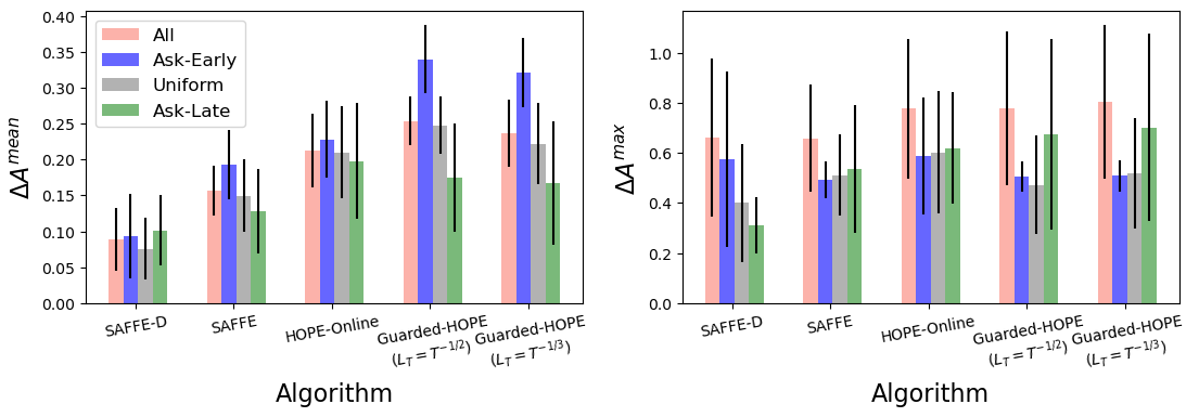
We investigate whether SAFFE-D allocates to agents differently based on their arrival or demand patterns. We consider agents with expected arrivals over the horizon , and Normal demands with , and budget size . Under the Non-symmetric Arrivals setting, we compare the agents’ allocations for each algorithm with respect to the Hindsight allocations in Fig. 3. In this setting, agents have different likelihoods of arriving over the horizon. We observe that despite being optimized for the log-NSW objective, SAFFE-D outperforms all other algorithms on average, and is more uniform across the three groups compared to SAFFE and Guarded-HOPE which favor the Ask-Late agents. In terms of the worst-case agent, SAFFE outperforms all other methods and has similar across all three groups. The algorithms are compared under the Non-symmetric Demands setting in Appendix K.2.
| Log-NSW () | Utilization % () | () | () | |
|---|---|---|---|---|
| Hindsight | 236.5710.21 | 100.00.0 | ||
| SAFFE-D () | 235.9110.26 | 99.451.5 | 0.050.02 | 0.450.23 |
| SAFFE-D () | 234.1210.67 | 97.863.5 | 0.090.03 | 0.650.22 |
| SAFFE () | 232.8910.91 | 95.774.5 | 0.110.03 | 0.690.21 |
6.3 Sensitivity to Estimation Errors
We investigate how sensitive the algorithms are to estimation errors by scaling each agent’s mean estimate at each step as , where denotes the noise level. Fig. 2(b) shows the change in performance as we vary the noise level from to , for the Symmetric setting with agents, expected per-agent arrivals, , and budget . We observe that SAFFE-D is robust to mean estimation noise while all other algorithms are impacted. This results from the discounting term in SAFFE-D, for which the hyper-parameter can be tuned to the estimation errors. However, when over-estimating the future demands, SAFFE and other methods will be initially more conservative which can lead to lower utilization and less fair allocations due to the leftover budget. When under-estimating the expected demands, they use the budget more greedily earlier on and deplete the budget sooner, resulting in less allocations to agents arriving later (especially in Gaurded-HOPE).
6.4 Choice of for SAFFE-D
The discounting term in SAFFE-D uses the confidence in estimates to improve the performance of SAFFE by balancing the budget between allocating now vs reserving for future arrivals. In Table 1, we compare the performance of SAFFE-D when using different discounting functions, i.e., constant or decreasing over the horizon. In both cases, the parameter is tuned to maximize Log-NSW. As expected from Sec. 4.2, the performance of SAFFE-D improves for decreasing over time. This is because the uncertainty in expected future demands reduces and the supplier can be less conservative when making allocation decisions.
| Per-agent Arrivals (Sparse) | Per-agent Arrivals (Dense) | ||||||||
|---|---|---|---|---|---|---|---|---|---|
| Log-NSW () | Utilization % () | () | () | Log-NSW () | Utilization % () | () | () | ||
| Hindsight | 35.741.23 | 100.00.0 | 47.372.20 | 100.00.0 | |||||
| RL Policy (SAC) | 35.111.20 | 95.630.49 | 0.13 0.01 | 0.43 0.01 | 47.002.20 | 98.300.45 | 0.120.01 | 0.340.02 | |
| SAFFE-D | 35.011.28 | 99.540.42 | 0.150.05 | 0.51 0.16 | 47.12 2.22 | 99.820.36 | 0.110.04 | 0.320.09 | |
| SAFFE | 34.771.19 | 92.740.41 | 0.160.02 | 0.530.03 | 46.872.15 | 97.140.43 | 0.120.02 | 0.350.03 | |
| Log-NSW () | Utilization % () | () | () | Log-NSW () | Utilization % () | () | () | ||
|---|---|---|---|---|---|---|---|---|---|
| Hindsight | 42.720.00 | 100.00.0 | 35.240.94 | 100.00.0 | |||||
| SAFFE-D | 42.720.00 | 100.00.0 | 0 | 0 | 35.160.94 | 100.00.0 | 0.060.04 | 0.170.14 | |
| SAFFE | 42.720.02 | 99.980.15 | 0.010.01 | 0.010.03 | 34.821.10 | 99.162.94 | 0.170.08 | 0.370.16 | |
| HOPE-Online | 42.710.02 | 99.980.15 | 0.100.04 | 0.040.01 | 34.441.10 | 99.103.03 | 0.270.06 | 0.600.15 | |
| Guarded-HOPE () | 42.480.30 | 97.932.80 | 0.070.02 | 0.160.05 | 33.553.67 | 95.936.24 | 0.270.06 | 0.620.15 | |
| Guarded-HOPE () | 42.550.21 | 98.641.94 | 0.070.02 | 0.150.05 | 33.593.67 | 96.545.61 | 0.280.07 | 0.630.15 | |
6.5 Reinforcement Learning Results
We investigate learning an allocation strategy using RL under the Symmetric setting. We train the RL allocation policy without access to any demand distribution information (e.g., expectation). We consider agents, and varying budget size sampled from . We use the Soft Actor-Critic (SAC) Haarnoja et al. (2018a); Achiam (2018) method with automatic entropy tuning Haarnoja et al. (2018b) to learn a policy (See Appendix L). The results averaged over experiment rollouts for five random seeds are reported in Table 2, for two cases where we expect to have and per-agent arrivals. We observe that while the RL policy is not able to match the hindsight performance, it outperforms SAFFE-D and other approaches in terms of Log-NSW under sparse ( per-agent) arrivals. With denser ( per-agent) arrivals, the RL policy performs slightly worse than SAFFE-D while still outperforming others. These observations are in line with other experiments illustrating the close-to-optimal performance of SAFFE-D especially in settings with more arrivals.
6.6 Real Data
In contrast to the demand processes considered in previous experiments, in this case, we need to estimate the expected demands and their standard deviations. The efficiency and fairness metrics are reported in Table 3 for budget size . We observe that SAFFE-D is optimal, and SAFFE and HOPE-Online perform very close to Hindsight in terms of Utilization and Log-NSW. As shown in Fig. 4(c) in Appendix K.1, we expect that SAFFE-D achieves (close to) hindsight performance for dense agent arrivals as with the daily arrivals in this setting. In order to investigate less dense scenarios, we impose sparsity in the arrivals by erasing each arrival with probability . As observed in Table 3, SAFFE-D is no longer optimal but outperforms all other methods. Additional results are provided in Appendix K.3.
7 Related Work
Fair division is a classic problem extensively studied for settings involving single and multiple resources, divisible and indivisible resources, and under different fairness objectives Bretthauer and Shetty (1995); Katoh and Ibaraki (1998); Lee and Lee (2005); Patriksson (2008). In the online setting, which requires real-time decision-making, Walsh (2011); Kash et al. (2014) consider the cake cutting problem where agents interested in fixed divisible resources arrive and depart over time, while the goal in Aleksandrov et al. (2015); Zeng and Psomas (2020); He et al. (2019) is to allocate sequentially arriving indivisible resources to a fixed set of agents. A wide range of fairness metrics are used in the literature, including global fairness (e.g., utilitarian or egalitarian welfare) Kalinowski et al. (2013); Manshadi et al. (2021), individual measures Benade et al. (2018); Gupta and Kamble (2021); Sinclair et al. (2022) or probabilistic notions of fairness across groups of agents Donahue and Kleinberg (2020).
The most relevant work to ours are Lien et al. (2014); Sinclair et al. (2020, 2022), which study the online allocation of divisible resources to agents with stochastic demands. Lien et al. (2014) proposes equitable policies that maximize the minimum agent utility, while Sinclair et al. (2020, 2022) use approximate individual fairness notions. Motivated by the food-bank allocation problem, Sinclair et al. (2020, 2022) assume one request per agent, where the requests are restricted to a finite set of values. The algorithm proposed in Sinclair et al. (2022) improves upon Sinclair et al. (2020) and achieves a trade-off between a measure of fairness (envy-freeness) and resource leftover using concentration arguments on the optimal NSW solution. In our work, we study a more general setup where agents can arrive simultaneously and several times over the horizon and we do not restrict agent demand sizes. Our goal is to be fair to the agents considering all their allocations over the horizon under the NSW objective in hindsight.
8 Conclusions
This paper studies the problem of fair resource allocation in the sequential setting, and mathematically formulates the NSW fairness objective under the MDP framework. With the goal to maximize the return in the MDP, we propose SAFFE-D, a new algorithm that enjoys a worst-case theoretical sub-optimality bound. Through extensive experiments, we show that SAFFE-D significantly outperforms existing approaches, and effectively balances the fraction of budget that should be used at each step versus preserved for the future. Empirical results under various demand processes demonstrate the superiority of SAFFE-D for different budget sizes, number of agents, and time horizons, especially in settings with dense arrivals. The uncertainty-based discount in SAFFE-D also improves the robustness of allocations to errors in future demand estimations. Future work includes exploring learning-based allocation policies, learning the optimal in SAFFE-D, and extensions to settings with strategic agents.
Disclaimer
This paper was prepared for informational purposes in part by the Artificial Intelligence Research group of JPMorgan Chase & Coȧnd its affiliates (“JP Morgan”), and is not a product of the Research Department of JP Morgan. JP Morgan makes no representation and warranty whatsoever and disclaims all liability, for the completeness, accuracy or reliability of the information contained herein. This document is not intended as investment research or investment advice, or a recommendation, offer or solicitation for the purchase or sale of any security, financial instrument, financial product or service, or to be used in any way for evaluating the merits of participating in any transaction, and shall not constitute a solicitation under any jurisdiction or to any person, if such solicitation under such jurisdiction or to such person would be unlawful.
References
- Abid et al. [2020] Adnan Abid, Muhammad Faraz Manzoor, Muhammad Shoaib Farooq, Uzma Farooq, and Muzammil Hussain. Challenges and issues of resource allocation techniques in cloud computing. KSII Transactions on Internet and Information Systems (TIIS), 14(7):2815–2839, 2020.
- Achiam [2018] Joshua Achiam. Spinning Up in Deep Reinforcement Learning. 2018.
- Aleksandrov et al. [2015] Martin Damyanov Aleksandrov, Haris Aziz, Serge Gaspers, and Toby Walsh. Online fair division: Analysing a food bank problem. In Twenty-Fourth International Joint Conference on Artificial Intelligence, 2015.
- Balasubramanian et al. [2007] Aruna Balasubramanian, Brian Levine, and Arun Venkataramani. Dtn routing as a resource allocation problem. pages 373–384, 2007.
- Bellman [1966] Richard Bellman. Dynamic programming. Science, 153(3731):34–37, 1966.
- Benade et al. [2018] Gerdus Benade, Aleksandr M Kazachkov, Ariel D Procaccia, and Christos-Alexandros Psomas. How to make envy vanish over time. In Proceedings of the 2018 ACM Conference on Economics and Computation, pages 593–610, 2018.
- Bretthauer and Shetty [1995] Kurt M Bretthauer and Bala Shetty. The nonlinear resource allocation problem. Operations research, 43(4):670–683, 1995.
- Cohen et al. [1965] Kalman J Cohen, Richard Michael Cyert, et al. Theory of the firm; resource allocation in a market economy. Prentice-Hall International Series in Management (EUA), 1965.
- Donahue and Kleinberg [2020] Kate Donahue and Jon Kleinberg. Fairness and utilization in allocating resources with uncertain demand. In Proceedings of the 2020 conference on fairness, accountability, and transparency, pages 658–668, 2020.
- Eisenberg and Gale [1959] Edmund Eisenberg and David Gale. Consensus of subjective probabilities: The pari-mutuel method. The Annals of Mathematical Statistics, 30(1):165–168, 1959.
- Eisenberg [1961] Edmund Eisenberg. Aggregation of utility functions. Management Science, 7(4):337–350, 1961.
- Furukawa [1972] Nagata Furukawa. Markovian decision processes with compact action spaces. The Annals of Mathematical Statistics, 43(5):1612–1622, 1972.
- Gallego et al. [2015] Guillermo Gallego, Anran Li, Van-Anh Truong, and Xinshang Wang. Online resource allocation with customer choice. arXiv preprint arXiv:1511.01837, 2015.
- Gupta and Kamble [2021] Swati Gupta and Vijay Kamble. Individual fairness in hindsight. J. Mach. Learn. Res., 22(144):1–35, 2021.
- Haarnoja et al. [2018a] Tuomas Haarnoja, Aurick Zhou, Pieter Abbeel, and Sergey Levine. Soft actor-critic: Off-policy maximum entropy deep reinforcement learning with a stochastic actor. In Proceedings of the 35th International Conference on Machine Learning, volume 80, pages 1856–1865, 2018.
- Haarnoja et al. [2018b] Tuomas Haarnoja, Aurick Zhou, Kristian Hartikainen, George Tucker, Sehoon Ha, Jie Tan, Vikash Kumar, Henry Zhu, Abhishek Gupta, Pieter Abbeel, and Sergey Levine. Soft actor-critic algorithms and applications. arXiv preprint, arXiv:1812.05905, 2018.
- He et al. [2019] Jiafan He, Ariel D Procaccia, CA Psomas, and David Zeng. Achieving a fairer future by changing the past. IJCAI’19, 2019.
- Kalinowski et al. [2013] Thomas Kalinowski, Nina Nardoytska, and Toby Walsh. A social welfare optimal sequential allocation procedure. arXiv preprint arXiv:1304.5892, 2013.
- Kaneko and Nakamura [1979] Mamoru Kaneko and Kenjiro Nakamura. The nash social welfare function. Econometrica: Journal of the Econometric Society, pages 423–435, 1979.
- Kash et al. [2014] Ian Kash, Ariel D Procaccia, and Nisarg Shah. No agent left behind: Dynamic fair division of multiple resources. Journal of Artificial Intelligence Research, 51:579–603, 2014.
- Katoh and Ibaraki [1998] Naoki Katoh and Toshihide Ibaraki. Resource allocation problems. Handbook of combinatorial optimization, pages 905–1006, 1998.
- Kumar et al. [1995] Nirmalya Kumar, Lisa K Scheer, and Jan-Benedict EM Steenkamp. The effects of supplier fairness on vulnerable resellers. Journal of marketing research, 32(1):54–65, 1995.
- Lee and Lee [2005] Zne-Jung Lee and Chou-Yuan Lee. A hybrid search algorithm with heuristics for resource allocation problem. Information sciences, 173(1-3):155–167, 2005.
- Lien et al. [2014] Robert W Lien, Seyed MR Iravani, and Karen R Smilowitz. Sequential resource allocation for nonprofit operations. Operations Research, 62(2):301–317, 2014.
- Manshadi et al. [2021] Vahideh Manshadi, Rad Niazadeh, and Scott Rodilitz. Fair dynamic rationing. In Proceedings of the 22nd ACM Conference on Economics and Computation, pages 694–695, 2021.
- Nair et al. [2018] Arun Sukumaran Nair, Tareq Hossen, Mitch Campion, Daisy Flora Selvaraj, Neena Goveas, Naima Kaabouch, and Prakash Ranganathan. Multi-agent systems for resource allocation and scheduling in a smart grid. Technology and Economics of Smart Grids and Sustainable Energy, 3(1):1–15, 2018.
- Nash [1950] John F Nash. The bargaining problem. Econometrica: Journal of the econometric society, pages 155–162, 1950.
- Patriksson [2008] Michael Patriksson. A survey on the continuous nonlinear resource allocation problem. European Journal of Operational Research, 185(1):1–46, 2008.
- Sinclair et al. [2020] Sean R Sinclair, Gauri Jain, Siddhartha Banerjee, and Christina Lee Yu. Sequential fair allocation of limited resources under stochastic demands. arXiv preprint arXiv:2011.14382, 2020.
- Sinclair et al. [2022] Sean R Sinclair, Siddhartha Banerjee, and Christina Lee Yu. Sequential fair allocation: Achieving the optimal envy-efficiency tradeoff curve. In Abstract Proceedings of the 2022 ACM SIGMETRICS/IFIP PERFORMANCE Joint International Conference on Measurement and Modeling of Computer Systems, pages 95–96, 2022.
- Varian [1973] Hal R Varian. Equity, envy, and efficiency. 1973.
- Walsh [2011] Toby Walsh. Online cake cutting. In International Conference on Algorithmic Decision Theory, pages 292–305. Springer, 2011.
- Yi et al. [2016] Peng Yi, Yiguang Hong, and Feng Liu. Initialization-free distributed algorithms for optimal resource allocation with feasibility constraints and application to economic dispatch of power systems. Automatica, 74:259–269, 2016.
- Yilmaz et al. [2004] Cengiz Yilmaz, Bulent Sezen, and Ebru Tumer Kabadayı. Supplier fairness as a mediating factor in the supplier performance–reseller satisfaction relationship. Journal of Business Research, 57(8):854–863, 2004.
- Zeng and Psomas [2020] David Zeng and Alexandros Psomas. Fairness-efficiency tradeoffs in dynamic fair division. In Proceedings of the 21st ACM Conference on Economics and Computation, pages 911–912, 2020.
Sequential Fair Resource Allocation under a Markov Decision Process Framework
Supplementary Materials
Appendix A Multiple-Resource Setting
The setting in this paper can be easily extended to the supplier having divisible resources, where resource has a limited budget of size , and . At time , agent ’s demands i denoted by , and the supplier’s allocation is . For multiple resources, , where denotes the per-unit value that agent associates to each resource,
| (19) |
While we present the paper in terms of a single resource, all algorithms and proofs can be extend to the multiple-resource setting. In this case, the optimal allocation in hindsight or the sequential setting will not have closed-form solutions as in the water-filling algorithm, but can be computed using convex optimization techniques.
Appendix B Existence of Optimal Policy
The state space of the MDP is continuous, the action space is continuous and state-dependent, and the reward is bounded and continuous due to the constant in Eq. (8). As a result of Furukawa [1972][Theorem 4.2], a stationary optimal policy is known to exist.
If we restrict the action space to allocations that satisfy for all and , the reward at step (7) becomes
| (20) |
where denotes the cumulative allocated resources to agent till time . At time step , maximizes which does not depend on future allocations. The optimal allocation can be directly computed from since there is no uncertainty about future demands. Then, the optimal policy for all can be derived by recursively solving (10) backward in time. This quickly becomes computationally intractable, which motivates us to find alternative solutions that trade-off sub-optimality for computational efficiency.
Appendix C Water-Filling Algorithm with Past Allocations
Algorithm 3 extends the water-filling algorithm presented in Algorithm 1 for agents with different weights to a setting where each agent may have past allocations denoted by . This algorithm is used as a base algorithm in SAFFE (Algorithm 2) to compute the allocations during each time step based on past allocations, and current and expected future demands. In line 3, the agents are ordered according to their demands, past allocations and weights. This ordering determines which agent is used to compute the water-level . For each selected agent , the condition in line 6 determines whether there is enough budget to fully satisfy agent ’s demand . If there is enough budget, agent receives its full request (line 10) and the supplier moves on to the next agent in order. Otherwise, the available budget is fully divided among the remaining agents (line 8) according to a water-level computed in line 7. The water-level accounts for the agent’s past allocations as well as their weights.
Appendix D SAFFE-Discounted vs SAFFE-Oracle
Under mild assumptions on the distribution of demands, we can quantify the distance between SAFFE-D and SAFFE-Oracle allocations using concentration inequalities on the deviation of future demands from their expected value. Let us define
| (21) | |||
| (22) |
For simplicity assume that agent ’s demands are i.i.d (this assumption can be relaxed see Remark 2). Then, for , with probability at least , based on Chebyshev’s inequality we have
| (23) |
We further assume that all agents have equal , but their expectations might differ (the assumption simplifies the presentation, and is not crucial). We first present the worst-case scenario bound, where we allow highly unbalanced future demands for different agents, i.e. there is an agent such that for all other agents .
Theorem 2 (Unbalanced demands bound).
Let and denote allocations by SAFFE-D for and SAFFE-Oracle, respectively. Then, for all agents we have
with probability at least .
Proof.
The detailed proof is in Appendix E. Intuitively, the discrepancy scales with the number of agents, since if all agnets submit demands according to their upper bound , then the water-level moves so that their SAFFE-Oracle allocations increase compared to SAFFE-Oracle with , which happens on the account of agent who now gets less. Finally, using (23) completes the proof, as we can translate the discrepancy between SAFFE-Oracle with and to that between SAFFE-D and SAFFE-Oracle with . ∎
Remark 2.
The equal standard deviation assumption that for any two agents and , we have is used in the proofs only to simplify . Thus, the assumption can be removed.
In order to move beyond the worst-case scenario of highly unbalanced request distributions, we now assume that all agents have the same and , e.g. if their demands are from the same distribution, the discrepancy between allocations scales better.
Theorem 3 (Balanced demands bound).
If for any two agents and we have the same bounds in (23), i.e. and , then for all agents , with probability at least , we have
Appendix E Detailed Proof of Theorem 2
Lemma 1 (Chebyshev’s inequality).
For a random variable with finite expectation and a finite non-zero variance, we have
In particular, under the assumption from Appendix D that agent ’s requests are i.i.d, Chebyshev’s inequality gives us that Eq. (23) holds with probability . Note however that the assumption is not crucial, and in a more general case we would have
and
See also Remark 2 on how the assumption on equal standard deviations for any two agents and is not crucial for the analysis.
We proceed as follows. First, we state the result for SAFFE-Oracle in the unbalanced demands regime, i.e. when there is an agent such that for all . Then, we state the result for the case of balanced demands, i.e. when and for any two and . Finally, we present the proof for both results.
Lemma 2 (Unbalanced demands SAFFE-Oracle).
Let and denote the allocations of SAFFE-Oracle with and , respectively. Then for all agents we have
| (24) |
Lemma 3 (Balanced demands SAFFE-Oracle).
Let and denote the allocations of SAFFE-Oracle with and , respectively. Then we have
| (25) |
Case .
Agents whose lower bound demands are fully filled by the lower bound solution with might increase the water-level when submitting larger demands, which will cause other agents to have smaller in comparison to . In the worst-case scenario, where agent ’s lower bound demand is greater than all other agents’ upper bound demands, the difference can be at most
i.e., agent has to compensate for the excess demands of all other agents. If is equal for all agents, the difference in the worst-case scenario is at most , which leads to a difference between of at most as a consequence of Lemma 4.
On the other hand if instead of the worst-case scenario we assume that and are the same for all agents (e.g. same demand distributions), then the water-level would not move in SAFFE using in comparison to SAFFE using , and thus there would be no change in the allocations resulting from the two problems.
Case .
There is enough budget to satisfy all agents’ demands under the lower bound constraint but not eoug budget under the upper bound one. Compared to , in the worst-case scenario, can decrease by at most
where agent ’s lower bound demand is larger than any other agents’ upper bound demands, and therefore, the water-filling algorithm will satisfy the upper bound demands of all other agents on the account of agent . If all agents have equal , in the worst-case scenario, the difference is again at most . Following Lemma 4, this leads to a difference of at most between and .
Case .
There is enough budget to satisfy all agents’ demands even under the upper bound, so the difference between and is purely driven by the difference between lower and upper bound demands, i.e. it equals which is . Following Lemma 4, this leads to a difference of at most between and . ∎
Lemma 4.
If , then we have
Proof.
Firstly, let us note that
and hence we have
where in the last inequality we use
Thus
∎
Appendix F SAFFE-Oracle Matches Hindsight
In Appendix D, we have upper bounded the discrepancy between the allocations of SAFFE-D and SAFFE-Oracle. Our next step is to show that SAFFE-Oracle achieves the optimal allocations in hindsight.
Theorem 4.
SAFFE-Oracle achieves optimal allocations in hindsight, i.e. for all we have , where is the solution to the Eisenber-Gale program (11).
Proof.
See Appendix G for a detailed proof, which relies on the following observations: 1) For , total allocations for the current step and the reserved allocations for the future , equals the solution of (11), and 2) SAFFE-Oracle fully distributes the total reserved allocations for future by the end of the horizon . ∎
Appendix G Detailed Proof of Theorem 4
Lemma 5.
At t=1, the solution to the SAFFE-Oracle problem coincides with the solution to the Eisenber-Gale program (11) i.e. .
Proof.
At , SAFFE-Oracle solves the following problem
| s.t. |
This is equivalent to problem (11) with , and hence, we have . ∎
Lemma 6.
With SAFFE-Oracle, for any agent we have
i.e. its future allocation from the first round is allocated in full by the end of the round.
Proof.
First, we prove that for we have
i.e. the past plus future allocation from the previous step is preserved in the following step. Recall that in each step we are solving
| (26) | ||||
| s.t. |
where the sequence of future demands is known to the oracle. It is easy to see that
because the constraints in step are tighter. If this didn’t hold, the previous round solution would not be the maximizing solution in step . It remains to note that can achieve its upper bound, because compared to the previous step , the remaining budget was reduced by exactly
Therefore,
satisifes the constraints. This means that , i.e., the current plus future allocation in step equals its counterpart in step minus the allocation in step . In particular, we get
| (27) | ||||
| (28) | ||||
| (29) | ||||
| (30) | ||||
| (31) | ||||
| (32) |
and in general we have
| (33) |
and
| (34) |
∎
Appendix H Detailed Proof of Theorem 1
Proof of Theorem 1.
Firstly, let us note that Theorem 4 guarantees that
as SAFFE-Oracle achieves the hindsight solution. It remains to employ Theorems 2 and 3 together with the triangle inequality in order to obtain an upper bound on the right hand side. In the case of unbalanced demands, this results in . In the case of balanced demands, we have ∎
Remark 3.
As , Theorem 1 also provides an upper bound on .
Appendix I SAFFE as a generalization of HOPE-Online
The heuristic algorithm HOPE-Online in Sinclair et al. [2020] coincides with SAFFE under a simplified demand process. HOPE-Online is designed for a setting where the supplier visits a set of agents sequentially in order. SAFFE generalizes the allocation algorithm to a setup where agents can arrive simultaneously and several times over the horizon . Similar to SAFFE-D which improves SAFFE using the uncertainty of future demand estimates, Guarded-HOPE proposed in Sinclair et al. [2022] improves HOPE-Online and achieves the correct trade-off between a measure of fairness (envy-freeness) and resource leftover by learning a “lower guardrail” on the optimal solution in hindsight. We highlight that Guarded-HOPE is designed for the setting where agents are not making repeated demands over the horizon i.e. each individual agent has a request at most once during the horizon. In that sense, our SAFFE and SAFFE-D represent generalizations as we allow for agents with multiple demands. In our analysis of the optimality of SAFFE-D, we rely on concentration inequalities for deviation of future demands from their expected values, which is in spirit similar to the optimality analysis of the guardrail approach in Sinclair et al. [2022].
Appendix J Extension of Guarded-HOPE to Our Setting
Since Guarded-HOPE was designed for a setting where in each time-step a number of individuals of the same type arrive, we slightly modify it to be applicable to our setting in Algorithm 4. The key components of the algorithm are the upper and lower guardrails defined in lines 7 and 10. Specifically, are high-confidence lower and upper bounds on the future demands, and , which Sinclair et al. [2020] refers to as upper and lower guardrails, respectively, are the optimal hindsight allocations under . When the demands are revealed in time step , the condition in line 13 first checks if the budget is insufficient to even allow an allocation according to the lower guardrail. If so, the budget is allocated right away and none is reserved. The condition in line 15 checks if the current demands can be allocated according to the upper guardrail assuming that the remaining budget is still enough to allow for allocations according to the lower guardrail for anticipated future demands. If so, the the upper guardrail is allocated to the agents with demands at the current step. Otherwise, the lower guardrail is allocated.
Appendix K Additional Experiments
K.1 Scaling System Parameters
SAFFE-D is compared to the baselines in terms of utilization and fairness metrics in Fig. 4, as different system parameters vary. Unless otherwise stated, the settings have agents, budget size , time horizon , and there are expected arrivals per-agent. In all experiments, we observe that SAFFE-D is more efficient and more fair compared to other methods, i.e., it achieves higher utilization, and lower Log-NSW, and . In Fig. 4(a), we observe that as the number of agents increases over the same horizon, the algorithms initially achieve higher utilization and lower Log-NSW, which eventually levels out. However, in terms of fairness which measures the allocation difference with respect to hindsight for the worst agent, SAFEE-D is the least affected across different number of agents, while all other algorithms become worse. Fig. 4(b) shows the metrics for varying horizon while having the same number of expected arrivals, i.e., when the arrivals are more spread out across time. In this setting, utilization and fairness metrics seem relatively unaffected across all methods.
In Fig. 4(c), we compare the algorithms as the number of arrivals over the horizon increases. We observe that SAFFE-D is able to use all the budget and match the fair hindsight allocations when it is expected to have more than arrivals per-agent over . SAFFE is able to match the performance of SAFFE-D in terms of utilization and Log-NSW as the arrivals become denser. As discussed in Appendix I, HOPE-Online and Guarded-HOPE are designed for settings with a single per-agent arrival. As expected, when there are several arrivals per agents, they are not able to match SAFFE-D or SAFFE since they do not account for an agent’s past allocations when distributing the budget.


K.2 Non-Symmetric Demands
Fig. 5 shows how SAFFE-D compares to other baselines in terms of allocations using the Non-symmetric Demands Setting, where some agents request larger demands earlier, while others have larger requests later or have no preference. We observe that SAFFE-D and SAFFE achieve lower , and have low variability across the groups on average. When considering the worst-case agent, SAFFE-D is less fair to agents that have larger demands earlier in the horizon, as it reserves the budget early on accounting for future expected demands. However, Uniform and More-Late agents receive allocations closer to hindsight compared to other algorithms.

K.3 Real Data
In order to study how SAFFE-D performs on real data with sparser arrivals over the horizon, we enforce less per-agent requests by erasing each arrival with probability . Since , setting corresponds to two weekly demands per store. As observed from Fig. 6, SAFFE-D outperforms the other methods in terms of efficiency and fairness. We remark that while with the uniform random erasures, we have imposed Bernoulli arrivals similar to the demand processes described in Sec. 6, the results presented here are based on the real demand sizes and reflect using imperfect estimates that are computed based on real data. However, further experiments on real datasets are needed to compare the performance of SAFFE-D under more general arrival processes that are correlated across time.

Appendix L Training of Reinforcement Learning Policy
We implement a variation of the Soft Actor-Critic method Haarnoja et al. [2018a] with clipped double-Q learning Achiam [2018] as well as automatic entropy Haarnoja et al. [2018b] tuning. We train the SAC policy for K episodes for random seeds, and then evaluate the checkpoints under another rollouts in order to compare with other baselines. We report the average performance with one standard deviation over the four metrics of Log-NSW, Utilization, and in Table 2.
The policy network architecture consists of three Fully Connected (FC) layers followed by one output layer, where each FC layer has 256 neurons with ReLU activation functions. Since the MDP state is time dependent, to prevent the input state vector size from growing over the time horizon during training, we represent the state vector as , where
Note that the state does not include any demand distribution information (e.g., expectation). We guarantee the step-wise budget constraint , by designing the output layer to have two heads: one head with a Sigmoid activation function, which outputs a scalar determining the step-wise budget utilization ratio ; and another head with a Softmax activation function, which outputs an allocation ratio vector, : over the agents. The final allocation for each agent is determined by .
We perform hyper-parameter tuning using a grid search over a set of candidates. The results in Table 2 are achieved by using the hyper-parameters summarized in Table 4.
| Parameter | Sparse | Dense |
|---|---|---|
| ( arrivals) | ( arrivals) | |
| Learning rate | ||
| Replay-buffer size | ||
| Batch size | 512 | 512 |
| Target smoothing coefficient | 0.005 | 0.005 |
| Update interval (step) | 5 | 1 |
| Update after (step) | ||
| Uniform-random action selection (step) |