Sensing Performance of Cooperative Joint Sensing-Communication UAV Network
Abstract
We propose a novel cooperative joint sensing-communication (JSC) unmanned aerial vehicle (UAV) network that can achieve downward-looking detection and transmit detection data simultaneously using the same time and frequency resources by exploiting the beam sharing scheme. The UAV network consists of a UAV that works as a fusion center (FCUAV) and multiple subordinate UAVs (SU). All UAVs fly at the fixed height. FCUAV integrates the sensing data of network and carries out downward-looking detection. SUs carry out downward-looking detection and transmit the sensing data to FCUAV. To achieve the beam sharing scheme, each UAV is equipped with a novel JSC antenna array that is composed of both the sensing subarray (SenA) and the communication subarray (ComA) in order to generate the sensing beam (SenB) and the communication beam (ComB) for detection and communication, respectively. SenB and ComB of each UAV share a total amount of radio power. Because of the spatial orthogonality of communication and sensing, SenB and ComB can be easily formed orthogonally. The upper bound of average cooperative sensing area (UB-ACSA) is defined as the metric to measure the sensing performance, which is related to the mutual sensing interference and the communication capacity. Numerical simulations prove the validity of the theoretical expressions for UB-ACSA of the network. The optimal number of UAVs and the optimal SenB power are identified under the total power constraint.
Index Terms:
Joint sensing-communication system, cooperative sensing, beam sharing, unmanned aerial vehicle network.I Introduction
Cooperative sensing unmanned aerial vehicle (UAV) network has been very promising in disaster rescue, surveillance, resource exploration, etc [2]. Due to unmanned feature and power restriction, UAVs need to achieve functions such as communication, environment sensing and flying status perception under load, volume and spectrum constraints. The utilization of the joint sensing-communication (JSC) technique on the UAV platform is a reasonable choice for the cooperative sensing UAV network, because it has advantages in load saving and spectrum reuse by sharing the same antennas, transceivers and spectrum to achieve sensing and communication [3]. With the integration of the sensing data from multiple UAVs using the JSC techniques, the sensing zone of the network will be extended far beyond the radio propagation limit of single sensing platform [4]. Thus, with limited spectrum for radar sensing and communication, the cooperative JSC UAV network can finish detecting a large area in much shorter time and gather more environment information than an individual UAV does, which makes the network be more agile and decide on a larger picture.
The achievement of the JSC technique gains increasingly sufficient fundamentals. The communication spectrum has gradually occupied the frequency band that was dedicated to radar at first [4]. Digital signal processing techniques have been widely utilized both in sensing and communication transceivers [4, 5]. Thus, the spectrum and hardwares that are separately designed for sensing and communication have great potential for convergence [3].
The strong need and potential for the joint design of communication and sensing has motivated a number of important studies in the JSC technique. The approaches to realize the JSC system can be divided into three categories: time sharing, waveform co-design and beam sharing. Time sharing scheme has the intrinsic disadvantage that it does not allow simultaneous operation of sensing and communication, which will lead to the loss of detection target [6]. As for waveform co-design scheme, the communication direction is rigidly constrained by sensing direction. Therefore, the freedom of communication is severely reduced [7, 8]. On the contrary, the beam sharing scheme allows simultaneous operation of sensing and communication using different beams, which can carry out communication and sensing as freely as possible [9, 10, 11, 1]. The beam sharing scheme is based on the beamforming technology that has solid fundamentals. Monzingo and Miller proposed maximum signal-to-noise ratio (SNR) beamforming to generate optimal beam with the existence of strong noise[12]. Frost proposed linearly-constrained minimum variance beamforming that can generate the beamforming vector with linear complexity [13]. Shi and Feng proposed a two-step iterative beamforming algorithm to achieve beamforming of high performance [14]. Another fundamental aspect in JSC implementation is the JSC waveform. Traditional sensing waveform design concentrates on the waveforms with desirable autocorrelation properties. Linear frequency modulated (LFM) pulse signal, i.e., “chirp” signal, is a typical sensing waveform [15]. Exploiting the high SNR characteristics of radar signal, a bio-inspired radio frequency (RF) steganography scheme that can conceal digital communication in linear chirp radar signals was proposed in [16]. Frequency modulated continuous wave (FMCW) is the typical continuous-wave sensing waveform [17]. In addition, the direct sequence spread spectrum (DSSS) waveform is also widely studied due to its features in information security and spectrum spread gains [18]. C. Sturm proposed an orthogonal-frequency-division-multiplexing (OFDM) symbol-based sensing processing technique to take advantage of temporal and frequency domain signal [19].
However, all the above works only study a single JSC unit or a single pair of JSC. Thus, in [1], we proposed a cooperative sensing performance metric of the JSC UAV network based on beam sharing scheme, but we were unable to put forward the proper antenna array model and beamforming algorithm. Moreover, we simplified the model by neglecting the mutual radar sensing interference and the guard distance between UAVs, which renders the proposed sensing performance metric less practical. Thus, in this paper, to enhance the concept of beam sharing JSC cooperative sensing UAV network we proposed in [1], we focus on the practical implementation of beam sharing JSC UAV network and further model the mutual sensing interference to analyze the sensing performance of cooperative JSC UAV network, which will offer guidance to the optimal deployment of the JSC UAV network, such as power allocation and the size of UAV network. The JSC UAV network consists of a UAV that works as the fusion center (FCUAV) and multiple subordinate UAVs (SU). All UAVs fly at the fixed height. UAVs carry out downward-looking sensing and integration of sensing data by generating a sensing beam (SenB) and a communication beam (ComB) with a novel JSC antenna array, respectively. The proper beamforming algorithm is also proposed. Because of the spatial orthogonality of communication and sensing, SenB and ComB can be easily formed orthogonally. SenB and ComB of each UAV share a total amount of available radio power. The average mutual sensing interference is modeled based on the radio propagation theory. The upper bound of average cooperative sensing area (UB-ACSA) is used to measure the cooperative sensing performance of the JSC UAV network [1], which is related to the mutual sensing interference and communication capacity. The main contributions of this paper are summarized as follows.
-
1.
We design a novel JSC antenna array and present a corresponding iterative beamforming algorithm that can flexibly form SenB and ComB using multi-layer circular array and linear array, respectively. Communication and sensing can operate simultaneously utilizing the proposed antenna array.
-
2.
We model the mutual sensing interference of the JSC UAV network, which can be used to evaluate the interference of the JSC UAV network.
-
3.
We define and formulate UB-ACSA of the JSC UAV network as the cooperative sensing performance metric, taking into consideration the average mutual sensing interference. After the formula of UB-ACSA is validated numerically, we obtain the optimal number of UAVs and power allocation ratio of sensing beam power to total available power.
The remaining parts of this paper are organized as follows. In Section II, we describe the cooperative JSC UAV network model, the beam sharing scheme, the design of JSC antenna, the corresponding beamforming algorithms, the JSC signal waveform, and the modeling of mutual sensing interference. Section III provides the closed-form expressions for minimum required signal-to-interference-and-noise ratio (SINR), the maximum sensing range of UAVs, maximum cooperative range (MCR), and UB-ACSA. Section IV formulates the outage capacity of the JSC UAV network as the communication performance metric. Subsequently, we provide the ultimate expression for MCR based on the outage capacity of the network. In section V, the numerical simulation of the previous theoretical results is presented. Section VI concludes this paper.
Notations: Bold uppercase letters denote matrices (i.e., M); bold lowercase letters denote column vectors (i.e., v); scalers are denoted by normal font (i.e., ); the entries of vectors or matrices are referred to with parenthesis, for instance, the th entry of vector v is , and the entry of the matrix M at the th row and th column is ; is the identity matrix with dimension . Also, matrix superscripts , and denote Hermitian transpose, complex conjugate and transpose, respectively. Besides, we use to denote inverse of matrix, to denote the pseudo-inverse of the matrix, to denote a diagonal matrix with the entries of v on the diagonal, to denote the expectation of random variable, and to denote the floor function.
| Symbol | Description |
| FCUAV | The UAV acting as fusion center |
| SU | Subordinate UAV |
| MCA | Maximum cooperating area |
| MCR | Maximum cooperating range, |
| SZ | Sensing zone |
| ACSA | Average cooperative sensing area |
| UB-ACSA | The upper bound of ACSA, |
| ComA | Communication subarray of JSC array |
| SenA | Sensing subarray of JSC array |
| ComB | Communication beam |
| SenB | Sensing beam |
| SPR | Sensing power ratio, |
| TxA | The transmitting antenna array of SenA |
| RxA | The receiving antenna array of SenA |
| S-C pair | The pair of FCUAV and an SU that is transmitting sensing data |
| STP | Successful transmission probability |
| The inner radius of MCA | |
| Maximum effective sensing range | |
| OFDM symbol-based radar processing gain | |
| The distance between SUi and FCUAV | |
| The flying height of UAVs |
II System Model
II-A Model of Cooperative JSC UAV Network
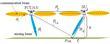
We consider a cooperative JSC UAV network that conducts downward-looking detection and detection data communication simultaneously. As illustrated in Fig. 1, the network consists of an FCUAV and SUs, where all UAVs hover within a constrained two-dimensional (2D) plane at a fixed altitude . Each UAV has an antenna array111All antenna elements are isotropic. that consists of a communication array (ComA) and a sensing array (SenA) to generate a ComB and a SenB, respectively. SenB is pointed downward to detect the targets on the ground (or the sea), and ComB is pointed to UAVs to transmit sensing data. Due to the significant difference between the sensing direction and the communication direction, ComB and SenB can be easily formed orthogonally and operate simultaneously to achieve beam sharing scheme. FCUAV integrates all the sensing data from SUs with ComB and detects targets simultaneously with SenB. SUs detect the targets with SenB while simultaneously transmitting the sensing data to FCUAV with ComB.
The antenna array of each UAV has available radio power , i.e., the sum of SenB power and ComB power is . The SenB power is given by
| (1) |
where is defined as the sensing power ratio (SPR). The ComB power is thus . OFDM waveform is adopted as the communication and sensing waveform to achieve joint communication and sensing [4]. Time division multiple access (TDMA) is adopted by the JSC UAV network to exploit the same frequency band to transmit sensing data. To ensure that FCUAV integrates the intact sensing data of each SU, the communication capacity between each SU and FCUAV has to be larger than the generating rate of sensing data. Therefore, the distance between FCUAV and each SU must be smaller than MCR, denoted by . Each UAV also has a guard radius for safety, within which no other UAVs can hover. Thus, SUs distribute within a concentric circle area centered at FCUAV, which is defined as the maximum cooperation area (MCA) whose inner and outer radii are and , respectively.
To satisfy the constraints on the false alarm rate and the detection probability for effective sensing [20], each UAV has to decrease the loss of sensing signal power and reduce interference to other UAVs in order to maintain the minimum SINR of sensing [21]. Thus, there is the maximum sensing range for each UAV, which is denoted by .
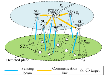
As shown in Fig. 1, the region on the ground that the JSC UAV network has to detect is defined as the detected plane. The region in the detected plane that can be effectively detected222i.e., the false alarm rate is below the maximum and detection probability is higher than the minimum. by a UAV is defined as the sensing zone (SZ) of the UAV. The maximum radius of SZ is determined by and . We propose the average union area of SZs of all UAVs to be the sensing performance metric of the JSC UAV network. The outage capacity of the links between SUs and FCUAV is defined as the communication performance metric of the JSC UAV network.
II-B Beam Sharing Scheme and Design of JSC Antenna Array
The beam sharing scheme is used to realize communication and sensing simultaneously. Let (,) be a certain direction in the three-dimensional (3D) space, where denotes the elevation angle and denotes the azimuth angle. ComA of each UAV generates ComB with elevation beamwidth333In this paper, the term “beamwidth” refers to the -3dB half-power beamwidth. and azimuth beamwidth . SenA of each UAV generates SenB with elevation beamwidth and azimuth beamwidth . Then the average directional gain of a 3D beam can be approximated by [11] [22]
| (2) |
where and are the azimuth beamwidth and elevation beamwidth, respectively.
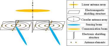
The antenna array designed to achieve beam sharing consists of two parts, as illustrated in Fig. 2. The upper linear subarray is ComA that has antenna elements with inter-distance half-wavelength. The lower subarray is SenA composed of two decoupled circular subarrays, where one is transmitting array (TxA) and the other is receiving array (RxA). TxA and RxA are used to generate transmitting SenB and receiving SenB, respectively. The electronic shielding plate is placed between two subarrays of SenA and the pulse response between two subarrays is also accurately measured to eliminate self-interference between TxA and RxA of SenA in real-time manner [23].
Two subarrays of SenA are used to solve the problem of minimum detection range by achieving simultaneous transmitting and receiving of radar sensing signal[21]. If SenA adopts only one subarray, then it has to arrange time slots for transmitting and receiving the radar signal. In this case, the radar echo can come back to SenA before the slot for receiving, and then the missing of the target will happen. Only when the distance between UAV and the target is larger than the minimum value can the target be possibly detected, which is inapplicable to the situation where the target is close to the JSC units. By contrast, if we adopt double subarrays to form SenA, then the radar sensing signal can be transmitted and received simultaneously. Thus, the problem of minimum detection range is solved.
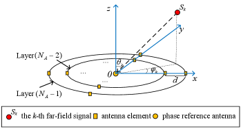
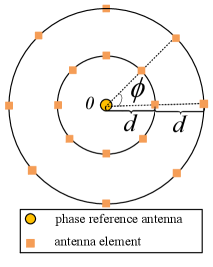
As illustrated in Fig. 3, SenA has antennas arranged in concentric circles. There are circles in each SenA, and we define each circle as a layer. From center to periphery, SenA has the 0th layer to the (1)th layer. Except for the 0th layer with only one antenna element that is the phase reference antenna (PhRefA), there are antenna elements in each layer, where is a positive integer.
Fig. 4 shows the adjacent layers of SenA. The distance between the antennas that locate at the same polar angle of adjacent layers is . Antennas in each layer locate at the evenly split angles, and are referred to as the th to the ()th antenna, anti-clockwise.
II-C Beamforming of JSC Antenna Array
II-C1 Beamforming of SenA
Assume that there are planar far-field signals arriving at SenA from different directions. The angle of arrival (AoA) of the th () signal is . We use to denote the set of AoAs of all signals.
Let be the th antenna in the th layer of SenA. The polar angle of is , where . For the th signal with AoA , the phase difference between and PhRefA is given by
| (3) |
where is the wavelength, and
Furthermore, the steering vector of SenA is
| (4) |
enumerating the phase differences between the PhRefA and all the other antenna elements of SenA. Then the steering matrix for far-field signals is .
The received signal vector for SenA is
| (5) |
where is the source signal vector of dimension , and is the additive white Gaussian noise (AWGN) with covariance matrix and zero mean.
Based on the least square (LS) error principle, the beamforming problem of SenA can be formulated as [14]
| (6) |
where is the normalized beamforming vector for SenA to generate SenB, and is the desired response, i.e.,
| (7) |
where
representing the desired amplitude response and desired phase response, respectively. Note that is a column vector of real values, and is a column vector of complex values with unit modulus.
Two-step iterative LS beamforming method is presented to generate high-performance beam given AoAs [14], as shown in Algorithm 1. First, we determine the desired AoAs, amplitude response and the corresponding steering matrix . Then we set the initial beamforming vector as and set the iteration time threshold as . If the iteration time is smaller than , then the phase response and the beamforming vector are updated iteratively. After the iteration time reaches or converges to a stable value, is the output as the beamforming vector for SenB beamforming. In Algorithm 1, brings out the vector where the th entry is the modulus of the th entry of ( can degrade to scalar), and is entry-wise division.
II-C2 Beamforming of ComA
Assume that there are planar far-field signals arriving at ComA. The th signal’s AoA is . Similar to SenA, the steering vector of ComA is
| (8) |
where is the distance between the adjacent antennas of ComA. Then we obtain the steering matrix of ComA as . Furthermore, the received signal of ComA can be expressed as , where is the source signal vector of dimension , and is AWGN with covariance matrix and zero mean. The objective for the ComA beamforming is given by
| (9) |
where and are the desired amplitude response and desired phase response of ComB, respectively. Note that is a column vector of real values, and is a column vector of complex values with unit modulus. Algorithm 1 is also applied to generate ComB. After iterations or converges to a stable value, the desired beamforming vector for ComB will be output.
II-D Signal Model of the JSC UAV Network
OFDM signal is adopted in the JSC UAV network to exploit its advantage of the frequency diversity and obtain high processing gain [19]. The baseband OFDM JSC signal is modeled as [19]
| (10) |
where is the number of OFDM symbols in one frame, is the number of subcarriers, is the transmit symbol on the th subcarrier of the th OFDM block, is the bandwidth of the JSC signal, is the baseband frequency of the th subcarrier, and is the duration time of each OFDM symbol that contains guard interval and the duration of OFDM block.
The phase difference between the transmitted and the received OFDM symbols is used to estimate the Doppler frequency shift and the time delay between the target and the UAV.
The Doppler shift results from the radial relative velocity between the UAV and the target, and can be presented as
| (11) |
where is the speed of light, is the carrier frequency of the OFDM signal, and is the radial relative velocity between UAV and the target. The time delay is expressed as
| (12) |
where is the distance between the target and the UAV. The complex ratio of the received to the transmitted OFDM signal is expressed as [19]
| (13) |
where is the entry of a matrix at the th row and the th column, is the received OFDM symbol corresponding to , and is the complex fading factor for the th subcarrier of the th OFDM symbol. The matrix form of (13) is given by
| (14) |
where , , , and .
By applying discrete Fourier transform (DFT) to each column of and inverse discrete Fourier transform (IDFT) to each row of , and can be obtained respectively.
Let denote the IDFT of the th row of , and denote the DFT of the th column of . The index corresponding to the peak of depends on and can be obtained by one-dimensional exhaustive search as follows [4]:
| (15) |
Similarly, the index corresponding to the peak of depends on and can be obtained by one-dimensional exhaustive search as follows [4]:
| (16) |
II-E Modeling of Mutual Sensing Interference
In order to model the mutual sensing interference, the power spectrum of the JSC OFDM signal needs to be considered first, which is the sum of the power spectra of subcarriers [24]. According to [24], the power spectrum of the th subcarrier is
| (18) |
where is the sampling cycle of the OFDM signal. The aggregate power spectrum of all subcarriers is noise-like [4]. For reasonable simplification, we assume that the transmitting power of the OFDM sensing signal concentrates in the baseband spectrum . UAVs receive the sensing interference power imposed by all other UAVs’ scattered sensing signals.
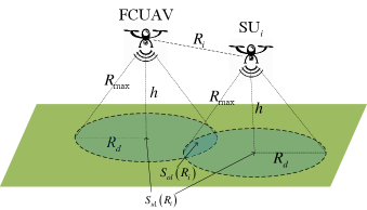
FCUAV is chosen as the reference to analyze the average sensing interference that a UAV receives from other UAVs. As illustrated in Fig. 5, denote as the distance between SUi and FCUAV,444 is an independently and identically distributed (i.i.d.) variable. as the intersection point between the SenB direction of SUi and SZ of SUi, as the distance between SUi and , as the distance between and FCUAV, and as the distance between and the projection point of SUi on SZ. Assuming that the interfering sensing signals are random due to the random scattering, the sensing interfering power imposed by SUi on FCUAV is formulated as [11, 25]
| (19) |
where and are the gains of transmitting and receiving sensing beams respectively, is the mean of radar cross section of target, is the wavelength of the carrier of JSC transceiver, and and are expressed as follows:
| (20) |
The maximal point of with regard to is , which is easily obtained by the first-order and the second-order derivative of versus . Thus, we set to obtain the upper bound of the average sensing interference imposed on FCUAV by SUi.
The expectation of sensing interference imposed on FCUAV by SUs can be upper-bounded by
| (21) |
III Sensing Performance Analysis of the JSC UAV Network
III-A Minimum Required SINR for Effective Sensing
As stated before, the power spectrum of OFDM signal is noise-like. Thus, the interference-and-noise imposed on sensing receiver of each UAV follows the Gaussian distribution, i.e., 555 is the Gaussian distribution with as mean and as variance., where is the thermal noise power.
The useful sensing signal power is
| (25) |
where denotes SINR of sensing, and is presented in (17). We can obtain the following detection problem:
| (26) |
where hypothesis is that there is a target in the direction of sensing beam, hypothesis is the opposite, and is the output signal of radar after processing OFDM symbols. The decision rule of whether there is a target in the sensing direction can be expressed as [20]
| (27) |
where is the decision threshold. When , the sensor accepts the hypothesis ; otherwise, the sensor accepts the hypothesis .
The false alarm rate and the detection probability are the metrics that have to be considered for detection [20], and are presented by
| (28) |
and
| (29) |
respectively, where is the monotonically decreasing Q-function [20]. According to (28), we have
| (30) |
where is the inverse function of Q-fucntion. By substituting (25) and (30) into (29), we can obtain as
| (31) |
III-B Maximum Sensing Range
According to [21], the maximum sensing range of UAV is
| (34) |
where is SPR, is the total available radio power, and are the transmitting and the receiving antenna gains of SenB respectively, is the carrier frequency of transceiver, is the mean radar cross section, is the aggregated power loss at the propagation medium, is given in (24), is the Boltzmann’s constant, is the noise figure of the receiver, is the bandwidth of JSC transceiver, and 290 K (in absolute temperature) is the standard temperature.
III-C Maximum Cooperative Range
The time that SU requires to transmit the sensing data to FCUAV is defined as the ratio of the amount of sensing data to the communication throughput, which is
| (35) |
where is the generating rate of the sensing data, is the detection time, and is the throughput of the communication link between FCUAV and SUi. With the increase of , decreases because the received ComB power decreases.
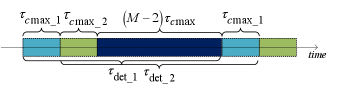
We adopt TDMA for SUs to transmit the sensing data to FCUAV. Each SU must transmit the sensing data in the assigned time slots of length . SUs carry out downward-looking detection constantly and transmit its sensing data in the assigned slots.
Fig. 6 illustrates the time slots allocated to SUs for transmitting sensing data to FCUAV. Let and denote the sensing slots and communication slots for SUi, respectively. All UAVs are provided with the same sensing time and transmission time . In order to ensure the consecutive detection of each UAV, we have
| (36) |
In this case, after SUi completes the sensing tasks in , the next slot for SUi to transmit sensing data comes again.
Based on (35), (36) and , we obtain . Thus, the distance between FCUAV and each SU is no larger than MCR, i.e.,
| (37) |
where is the inverse function of and will be presented in the next section.
III-D Cooperative Sensing Performance Analysis
We define an SU and FCUAV that are communicating sensing data as an S-C pair. As shown in Fig. 7, the radius of SZ of each UAV is formulated as
| (42) | ||||
| (43) | ||||
| (38) |
where is the step function666i.e., when there is , ; otherwise, .. The overlapped area between SZs of the S-C pair is
| (39) | ||||
Then, the union area of SZs of the S-C pair is
| (40) |
The expectation of , for , is defined as the sensing performance metric of the S-C pair, which is formulated as [1]
| (41) | ||||
where for , is the probability density function (PDF) of . Moreover, and are given in (42) and (43), respectively.
There are S-C pairs located in MCA. ACSA of the JSC UAV network is defined as the average union area of SZs of S-C pairs. Because it is extremely intractable to obtain an explicit expression of the average union area of a certain number of randomly distributed circle areas. For tractability, we merely subtract the overlapped sensing area between each SU and FCUAV to obtain the upper bound of ACSA (UB-ACSA) as the sensing performance metric of the JSC UAV network. UB-ACSA is obtained as [1]
| (44) |
where is the area of SZ of each UAV, and is the multiple random variables composed of the distances between SUs and FCUAV. Each element of is an i.i.d. variable.
UB-ACSA can be achieved when all SUs do not have overlapped SZs, which requires FCUAV to coordinate the trajectory of each SU. The larger UB-ACSA is, the better the sensing performance of the JSC UAV network is. The JSC UAV network can detect the zone with area of UB-ACSA in much shorter time than individual UAV can do. The overlapped SZs of SUs can be detected by different SUs from different directions, which can reduce the probability of false detection in the overlapped SZs.
IV Outage Capacity of the JSC UAV Network
In this section, we obtain the outage capacity as the metric of communication performance, as well as the ultimate expression of with respect to the number of UAVs and SPR.
IV-A Communication Channel Model
The power of communication signal received by FCUAV is
| (45) |
where is the power of ComB, is the path loss exponent, is the directional gain of the communication link, is the small scale fading factor that follows Rician distribution with Rician factor , and is the distance between the transmitter and FCUAV. We have , where and are the directional gains of transmitting ComB and receiving ComB, respectively. The PDF of is expressed as follows [26]:
| (46) |
where is the 0-th order modified Bessel function of the first kind, , is the normalized power, denotes the strong line-of-sight (LOS) power, and represents the multipath reflected power [27, 28, 29].
IV-B Successful Transmission Probability and Outage Capacity
The successful transmission probability (STP) is defined as the probability that the received SNR (or SINR) is larger than a threshold that is necessary for successful transmission [26],[30], i.e.,
| (47) |
where is AWGN of communication receiver. Since follows Rician distribution with Rician factor , STP is formulated as [27]
| (48) |
where is the first order Marcum Q-function. The outage probability is the complement of , i.e.,
| (49) |
The outage capacity is written as [30]
| (50) |
where is the available bandwidth of the JSC transceiver, is the maximum of , and is the SNR threshold that makes the outage probability equal to [30]. If , then the outage probability will be larger than . Combining (48), (49) and (50), we have
| (51) |
where is the inverse function of with regard to ,777As is a monotonically decreasing function of [31], the inverse function of the first order Marcum Q-function with regard to exists. If , then . and is the communication performance metric of the JSC UAV network.
V Numerical Results
In this section, numerical and Monte-Carlo simulations are conducted to verify the theoretical analysis in the previous sections and show the impact of the number of SUs and SPR on UB-ACSA. The parameters used in the simulations are listed in TABLE II [21],[29],[32].
| Parameter Items | Value | Description |
| W | The total available power | |
| 94 dB | The power of AWGN for communication | |
| 2 | The threshold for STP | |
| 8 | The gain of transmitting ComB | |
| 8 | The gain of receiving ComB | |
| 16 | The number of OFDM symbols in a frame | |
| 64 | The number of subcarriers | |
| 1024 | The processing gain of sensing | |
| 16 | The number of antennas of ComA | |
| 17 | The number of layers of SenA | |
| 16 | The number of antennas in each layer of SenA | |
| The maximum false alarm rate | ||
| 0.99999999 | The minimum detection probability | |
| 150 m | The flying height of UAVs | |
| 2.6 | The path loss exponent | |
| 0.1 | The maximum outage probability | |
| 24 GHz | The carrier frequency | |
| 1 | The average radar cross section | |
| 10 | The noise figure of receiver | |
| 290 K | The standard temperature | |
| 100 MHz | The bandwidth of transceiver | |
| 1 MB/s | The generating rate of sensing data | |
| 10 dB | The Rician factor | |
| 1 | The propagation loss |
Fig. 8 shows the normalized 3D beam pattern of SenB. The mainlobe gain of 3D SenB is at least 21dB higher than that of the sidelobes. The azimuth and elevation beamwidth of SenB are approximately 4.5 and 5 degrees, respectively. Therefore, the average gain of SenB is approximately 128 (in decimal), based on (2).
Fig. 9 shows the normalized 2D beam pattern of ComA. The mainlobe gain of ComB is at least 15 dB higher than that of the sidelobes. The elevation beamwidth of ComB is approximately 9 degrees. Besides, the azimuth beamwidth of ComB is 360 degrees. Thus, the average gain of ComB is approximately 8 (in decimal) according to (2).
Fig. 10 plots both analytical and simulation results of STP versus the transmission distance under different SPR. We can see that STP is a monotonically decreasing function of the transmission distance. We also see the transmission distance becomes smaller with the increase of SPR under the same STP constraint, because the ComB power decreases as SPR or transmission distance increases.
Fig. 11 presents the results of versus and . The target is at the distance of 500 m, and the maximum false alarm rate is 10-8. As is shown in Fig. 11, on the one hand, decreases sharply when increases to a certain value under given . This is because the increase of results in the decrease of and the increase of . On the other hand, when is given, first increases with the increase of . Then after the maximum point, decreases. This is because as increases, the power of SenB increases at first, increasing the SINR of sensing. After gets too large, the ComB power decreases, leading to the decrease of and increase of . Thus, when SINR of sensing is lower than , will decrease sharply with the deterioration of SINR. The decrease of is required to increase SINR of sensing when or increases.
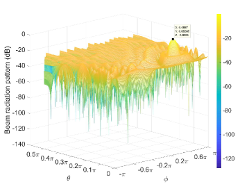
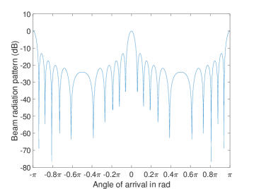
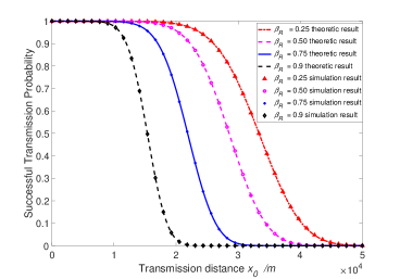
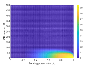
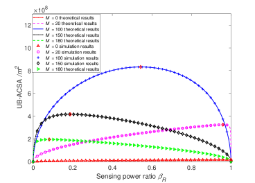
Fig. 12 plots both the analytical and simulation results of UB-ACSA changing versus , under different given . Each curve can be generally divided into three stages given . In the first stage where is low, the power of ComB is large. Then MCA is large enough for UAVs to expand the sensing zone. Thus, UB-ACSA increases with the increase of . When is too large, the second stage comes. In the second stage, after the maximum point, UB-ACSA decreases with the increase of , because the mutual sensing interference (i.e., ) will increase with the decrease of and the increase of the SenB power. Therefore, the maximum sensing range (i.e., ) decreases with the increase of in the second stage. When is so large that holds, the third stage appears. In the third stage, UB-ACSA decreases and converges to 0 m2, because is extremely large. Thus, in the third stage, it would be better to only deploy FCUAV to carry out the sensing mission than to deploy any other SUs. In Fig. 12, when the JSC UAV network contains 100 SUs, the maximum UB-ACSA is 8.32 m2, which is achieved when there is = 0.5430. With the above procedure, we can determine the optimal for each UAV given .
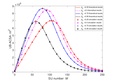
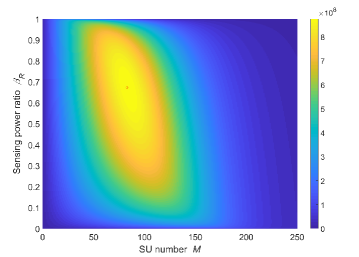
Fig. 13 demonstrates the analytical and simulation results of UB-ACSA changing versus under different . Each curve of UB-ACSA has three obvious stages. In the first stage where is relatively small, UB-ACSA increases with the increase of fast and linearly. This results from that is considerably large, because the communication capacity requirement for integrating the SUs’ sensing data is low. When gets too large, the second stage comes, where is much smaller. After reaching the maximum point of UB-ACSA, UB-ACSA decreases fast with the increase of , because keeps dropping down, gets larger fast, and the overlapped SZs get increasingly larger. If is so large that gets extremely small and becomes too large, then converges to 0 m. Therefore, UB-ACSA will become 0 m2 hereafter, which is the third stage. Moreover, fewer SUs are needed to reach the maximum UB-ACSA as increases, because if the given ComB power decreases, then fewer SUs can be supported to transmit the entire sensing data to FCUAV. Besides, fewer SUs can make be 0 m as increases, because the increase of the SenB power and decrease of lead to the increase of . In Fig. 13, when is 0.75, the optimal value of is 79, which makes UB-ACSA reach the maximum value, i.e., 8.672 m2. Using the above procedure, we can easily find the optimal to accomplish the maximum UB-ACSA, given the value of .
Fig. 14 presents the results of UB-ACSA changing versus and . On the one hand, when and are relatively small, the communication capacity is much larger than the requirement for sensing data integration, because the ComB power is considerably large, while the number of UAVs to integrate sensing data is too small. Therefore, the communication capacity for data integration is not completely exploited, i.e., UB-ACSA cannot reach the maximum value when and is small. On the other hand, too large will result in the decrease of UB-ACSA because of the decrease of . When is too large, also becomes quite small, and will become large enough to make decrease to a small value. As a result, when and are too large, UB-ACSA will decrease with the increase of and until UB-ACSA reduces to 0 m2. In Fig. 14, when 0.6741 and 83, UB-ACSA reaches the maximum value of 8.748 m2. In the above procedure, we can easily determine the optimal values of and to achieve the optimal UB-ACSA.
VI Conclusion
This work has put forward the average cooperative sensing area as performance metric of cooperative sensing in JSC UAV network. To achieve cooperative sensing of UAV network, we propose a novel design of JSC antenna array that consists of the communication subarray and sensing subarray and put forward relative beamforming algorithm. Further, the upper bound of mutual interference of sensing, the minimum required sensing SINR, the maximum sensing range and the maximum cooperative range that can allow SUs to transmit the sensing data to FCUAV successfully are derived. Further, the upper bound of average cooperative sensing area is derived as the tractable performance metric of cooperative sensing, which is related to SPR and the number of UAVs. SPR determines the maximum sensing range, the upper bound of mutual interference of sensing and the maximum cooperative range. The number of SUs determines the maximum cooperative range and the mutual interference of the sensing of UAVs. Finally, the optimal value of SPR and the number of UAVs to achieve the maximum UB-ACSA have been numerically determined. The results can guide the configuration of the JSC UAV cooperative sensing network.
Theorem 1.
A 2D uniform point process is generated within a concentric circle area whose inner radius and outer radius are and , respectively. The distance between a generated point and the center is denoted by . Let denote a constant parameter. Then the expectation of of is
Proof.
The cumulative density function of should be . Thus, the cumulative distribution function of ( and ) is
| (53) |
where . Then, the probability density function of is
| (54) |
where . Thus, the expectation of is
| (55) |
∎
References
- [1] X. Chen, Z. Wei, Z. Fang, H. Ma, Z. Feng, and H. Wu, “Performance of joint radar-communication enabled cooperative UAV network,” IEEE International Conference on Signal, Information and Data Processing 2019, pp. 1–4, Dec. 2019.
- [2] W. L. Teacy, J. Nie, S. McClean, and G. Parr, “Maintaining connectivity in UAV swarm sensing,” 2010 IEEE Globecom Workshops, pp. 1771–1776, Jan. 2011.
- [3] L. Han and K. Wu, “Joint wireless communication and radar sensing systems- state-of-the-art and future prospects,” IET Microwaves, Antennas & Propagation, vol. 7, no. 11, pp. 876–885, Aug. 2013.
- [4] C. Sturm and W. Wiesbeck, “Waveform design and signal processing aspects for fusion of wireless communications and radar sensing,” Proceedings of the IEEE, vol. 99, no. 7, pp. 1236–1259, May. 2011.
- [5] A. Gupta and R. K. Jha, “A survey of 5G network: Architecture and emerging technologies,” IEEE Access, vol. 3, pp. 1206–1232, May. 2015.
- [6] J. Moghaddasi and K. Wu, “Multifunctional transceiver for future radar sensing and radio communicating data-fusion platform,” IEEE Access, vol. 4, pp. 818–838, Feb. 2016.
- [7] J. Ellinger, Z. Zhang, Z. Wu, and M. C. Wicks, “Dual-use multicarrier waveform for radar detection and communication,” IEEE Transactions on Aerospace and Electronic Systems, vol. 54, no. 3, pp. 1265–1278, June 2018.
- [8] C. Shi, F. Wang, M. Sellathurai, J. Zhou, and S. Salous, “Power minimization-based robust OFDM radar waveform design for radar and communication systems in coexistence,” IEEE Transactions on Signal Processing, vol. 66, no. 5, pp. 1316–1330, Jan. 2018.
- [9] F. Liu, C. Masouros, A. Li, H. Sun, and L. Hanzo, “MU-MIMO communications with MIMO radar: From co-existence to joint transmission,” IEEE Transactions on Wireless Communications, vol. 17, no. 4, pp. 2755–2770, Feb. 2018.
- [10] P. M. McCormick, S. D. Blunt, and J. G. Metcalf, “Simultaneous radar and communications emissions from a common aperture, Part I: Theory,” 2017 IEEE Radar Conference, pp. 1685–1690, Jun. 2017.
- [11] M. A. Richards, “Fundamentals of radar signal processing,” Tata McGraw-Hill Education, 2005.
- [12] R. A. Monzingo and T. W. Miller, “Introduction to adaptive arrays,” Scitech publishing, 2004.
- [13] O. L. Frost, “An algorithm for linearly constrained adaptive array processing,” Proceedings of the IEEE, vol. 60, no. 8, pp. 926–935, 1972.
- [14] Z. Shi and Z. Feng, “A new array pattern synthesis algorithm using the two-step least-squares method,” IEEE signal processing letters, vol. 12, no. 3, pp. 250–253, Mar. 2005.
- [15] M. I. Skolnik, “Radar handbook,” McGraw–Hill, 1970.
- [16] W. M. Z. W. Zhiping Zhang, N. Michael J, “Bio-inspired RF steganography via linear chirp radar signals,” IEEE Communications Magazine, vol. 54, no. 6, pp. 82–86, June 2016.
- [17] A. G. Stove, “Linear FMCW radar techniques,” Radar and Signal Processing, IEE Proceedings F, vol. 139, no. 5, pp. 343–350, Oct. 1992.
- [18] F. E. Nathanson, J. P. Reilly, and M. N. Cohen, “Radar design principles-signal processing and the environment,” NASA STI/Recon Technical Report A, vol. 91, 1991.
- [19] C. Sturm, T. Zwick, W. Wiesbeck, and M. Braun, “Performance verification of symbol-based OFDM radar processing,” 2010 IEEE Radar Conference, pp. 60–63, May 2010.
- [20] B. C. Levy, “Principles of signal detection and parameter estimation,” Springer Science & Business Media, 2008.
- [21] M. A. Richards, J. Scheer, W. A. Holm, and W. L. Melvin, “Principles of modern radar,” Citeseer, 2010.
- [22] R. J. Mailloux, Phased array antenna handbook. Artech house, 2017.
- [23] Z. Zhang, X. Chai, K. Long, A. V. Vasilakos, and L. Hanzo, “Full duplex techniques for 5G networks: self-interference cancellation, protocol design, and relay selection,” IEEE Communications Magazine, vol. 53, no. 5, pp. 128–137, May 2015.
- [24] J. G. Proakis, M. Salehi, N. Zhou, and X. Li, “Communication systems engineering,” Prentice Hall New Jersey, vol. 2, 1994.
- [25] A. F. Molisch, “Wireless communications,” John Wiley & Sons, vol. 34, 2012.
- [26] X. Yuan, Z. Feng, W. Xu, W. Ni, J. A. Zhang, Z. Wei, and R. P. Liu, “Capacity analysis of UAV communications: Cases of random trajectories,” IEEE Transactions on Vehicular Technology, vol. 67, no. 8, pp. 7564–7576, Aug. 2018.
- [27] M. M. Azari, F. Rosas, K.-C. Chen, and S. Pollin, “Ultra reliable UAV communication using altitude and cooperation diversity,” IEEE Transactions on Communications, vol. 66, no. 1, pp. 330–344, Jan. 2018.
- [28] N. Goddemeier and C. Wietfeld, “Investigation of air-to-air channel characteristics and a UAV specific extension to the Rice model,” 2015 IEEE Globecom Workshops, pp. 1–5, Dec. 2015.
- [29] A. A. Khuwaja, Y. Chen, N. Zhao, M.-S. Alouini, and P. Dobbins, “A survey of channel modeling for UAV communications,” IEEE Communications Surveys Tutorials, Jul. 2018.
- [30] S. Zhalehpour, M. Uysal, O. A. Dobre, and T. Ngatched, “Outage capacity and throughput analysis of multiuser FSO systems,” 2015 IEEE 14th Canadian Workshop on Information Theory, Jul. 2015.
- [31] D. A. Shnidman, “The calculation of the probability of detection and the generalized marcum Q-function,” IEEE Transactions on Information Theory, vol. 35, no. 2, pp. 389–400, Mar. 1989.
- [32] V. Lakshmanan, “Overview of radar data compression,” Satellite Data Compression, Communications, and Archiving III, vol. 6683, Sep. 2007.