Semiclassical magnetotransport including the effects of the Berry curvature and Lorentz force
Abstract
In topological semimetals and insulators, negative longitudinal magnetoresistance and angle-dependent planar Hall effect have been reported arising from the Berry curvature. Using the Boltzmann transport theory, we present a closed-form expression for the nonequilibrium distribution function which includes both the effects of the Berry curvature and Lorentz force. Using this formulation, we obtain analytical expressions for conductivity and resistivity tensors in Weyl semimetals demonstrating a characteristic field dependence arising from the competition between the two effects.
I Introduction
In topological materials with a nonvanishing Berry curvature, the positive magnetoconductance has been observed experimentally in the presence of parallel electric and magnetic fields KIM2013 ; HUANG2015 ; XIONG2015 ; LI2015 ; LI2016a ; ZHANG2016 ; LI2016b ; ZHANG2016 ; ZHANG2017 ; WANG2012 ; HE2013 ; WANG2015 ; WIEDMANN2016 ; ARNOLD2016 ; BREUNIG2017 ; ASSAF2017 . This is a unique feature to topological materials that does not occur in conventional magnetotransport which only takes classical Lorentz force effect into account.
The prevailing explanation for the positive longitudinal magnetoconductance is the so-called chiral anomaly. In 1983, Nielsen and Ninomiya suggested the chiral anomaly in Weyl fermions under a strong magnetic field regime where the chiral zeroth Landau level creates a one-dimensional conducting channel that pumps electrons from one Weyl node to another NIELSEN1983 . In 2013, Son and Spivak discussed chiral anomaly in Weyl semimetals under weak external magnetic field using the semi-classical Boltzmann approach SON2013 . They argued the positive magnetoconductivity that scales quadratically in magnetic field is due to topological charge pumping. One can expect possible detection of chiral anomaly between the valleys, given that the intervalley scattering is negligible compared to the intravalley scattering SEKINE2017 . However, chiral anomaly cannot be responsible for observed positive magnetoconductivity in topological insulators (TIs) where chiral charges are not well defined WANG2012 ; HE2013 ; WANG2015 ; WIEDMANN2016 ; ARNOLD2016 ; BREUNIG2017 ; ASSAF2017 . In topological materials such as TIs DAI2017 and Weyl semimetals (WSMs) KIM2014 , it is suggested that the anomalous velocity induced by the non-trivial Berry curvature alone can generate an additional contribution to the conductivity that grows with the magnetic field.
To understand magnetotransport properties quantitatively, it is important to consider both the effects of the anomalous velocity due to the non-trivial Berry curvature and the classical Lorentz force effect. Most of the previous studies KIM2014 ; DAI2017 ; NANDY2017 have focused on the Berry curvature effect, while only a few took the Lorentz force into considerations in describing magnetotransport behaviors IMRAN2018 ; JOHANSSON2019 . In this paper, we revisit semiclassical treatment of magnetotransport in topological materials to shed more light on the origin of the observed positive magnetoconductivity. We present a general semiclassical formula for conductivity which fully incorporates the Berry curvature and the Lorentz force. From the Boltzmann transport equation, we obtain a closed-form expression for the nonequilibrium distribution function by solving the corresponding self-consistent equation. We then apply our formula to WSMs and express the magnetoconductivity in terms of dimensionless parameters characterizing magnetic fields associated with the Lorentz force and the Berry curvature, respectively.
II Semiclassical Boltzmann magnetotransport theory for topological materials
The semiclassical Boltzmann transport equation governs the time evolution of a non-equilibrium distribution function at position and momentum . It states that the time evolution of equals the probability rate of electrons being scattered in and out of the distribution, called the collision term :
| (1) |
In a homogeneous sample with a steady external perturbation, there are no position nor time dependence in the distribution function . Then, simplifies to
| (2) |
where we have included a subscript to the non-equilibrium distribution function to indicate that it is only a function of . In a simple relaxation time approximation, the collision integral is replaced by the ratio between the deviation from the equilibrium Fermi-Dirac distribution and the average time between successive collisions. Hence,
| (3) |
where . Here we assume a constant transport relaxation time in momentum and magnetic field for a given chemical potential. Note that when we fully consider the collision integral in the system with a nontrivial Berry curvature, the transport relaxation time may show a field dependent anisotropy induced by the coupling between the Berry curvature and magnetic field PARK2021 . However, in weak magnetic field regime, we can assume as a constant. Furthermore, when short-range scattering is dominant or charged impurities are fully screened, we can assume that does not depend on XIAO2005 ; Ashcroft1976 ; Ziman1960 .
Here we provide a closed-form expression for magnetoconductivity in the presence of both a non-trivial Berry curvature and the Lorentz force within the semiclassical Boltzmann approach. The semiclassical equations of motion for electrons with a charge in the presence of the Berry curvature are given by XIAO2010
| (4a) | ||||
| (4b) | ||||
where , is the unperturbed band energy, is an orbital magnetic moment that couple to the magnetic field and is the Berry curvature. It has been reported that disorder affects not only the carrier distribution but also the semiclassical equations of motion, generating a correction to the velocity proportional to the disorder strength ATENCIA2022 . In this work, we neglect this correction assuming a weak disorder potential for simplicity. In the presence of a magnetic field, and in Eq. (4) are coupled through the Lorentz force. Combining these two equations of motion, we have
| (5a) | ||||
| (5b) | ||||
where and represents the modified density of states in the phase space due to the Berry curvature effect XIAO2005 . The first term in the square bracket in Eq. (5b) corresponds to electric force due to an electric field and the second term represents Lorentz force due to a magnetic field . The last term is anomalous electromagnetic force due to the Berry curvature which leads to positive magnetoconductivity in topological materials.
Replacing according to the relaxation time approximation in Eq. (3), we have
| (6) |
Plugging Eq. (5) into Eq. (6), we get
| (7) | |||||
In previous studies DAI2017 ; KIM2014 ; NANDY2017 of magnetoconductivity and planar Hall conductivity in topological materials, Lorentz force effect has been often neglected. Therefore, in order to better understand positive longitudinal magnetoconductivity and angle-dependent planar Hall conductivity in topological materials, we take all the terms in Eq. (7) into consideration.
We can rewrite Eq. (7) in the following form:
| (8) |
where
| (9) |
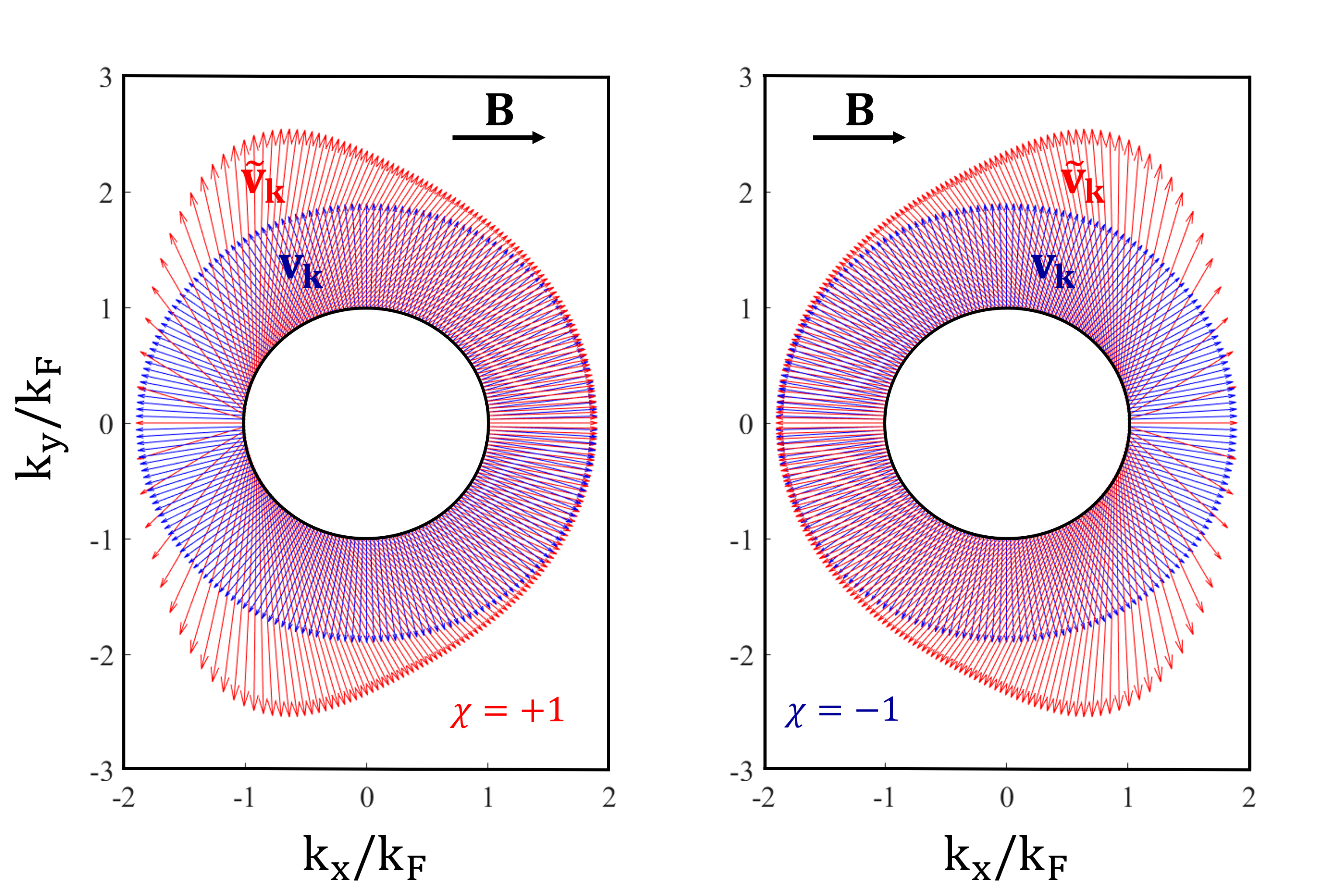
Figure 1 shows a schematic picture of in WSMs in the presence of a magnetic field . As shown in Fig. 1, is greater in magnitude than in all except when is parallel to giving . In general, it is this effect due to Berry curvature that leads to enhanced magnetoconductivity in topological materials.
Our goal now is to solve for in Eq. (8). We assume that a small deviation from the equilibrium distribution takes the form of where is some arbitrary vector that is independent of . Upon plugging into Eq. (8), we obtain
| (10) |
where is the inverse mass tensor. Factoring out,
| (11) |
From and Eq. (11), we obtain a self-consistent form of as
| (12) |
where
| (13) |
The solution for Eq. (12) can be obtained as
| (14) |
where is the magnetic field strength tensor (see Appendix A for a detailed derivation). Thus, we obtain
| (15) |
The current is therefore computed as
| (16) |
where is the direction in which we measure the current. Let us denote the current associated with as and that associated with as . From now on, we will only focus on the extrinsic contribution arising from scatterings.
Plugging Eq. (15) into and using relation, we finally arrive at
| (17) | |||||
where is the direction of an electric field.
Now let us assume that the mobility tensor is set to a constant for simplicity. Then in Eq. (14) becomes (see Appendix A)
| (18) |
Note that the obtained is consistent with the assumption that is independent of . Then is given by
| (19) |
Using Eq. (19), we finally obtain the following form for magnetoconductivity
The above form is a general expression of magnetoconductivity for topological materials including the Berry curvature and Lorentz force within the semiclassical regime under the assumption that in is independent of and the mobility tensor is a constant.
III Magnetotransport in Weyl semimetals
In this section, we study the magnetotransport properties of WSMs in three dimensions using a closed-form expression for magnetoconductivity Eq. (II) discussed in the previous section. For simplicity, we consider a single Weyl node described by the Hamiltonian which has isotropic linear dispersion, where are for the different chiralities of Weyl fermions and are the Pauli matrices.
III.1 Longitudinal magnetoconductivity
To investigate longitudinal magnetoconductivity in WSMs, without loss of generality, we set the electric and magnetic field orientations as and , respectively. Organizing terms in Eq. (II) in powers of and using Eq. (9),
| (21) |
where is a sum of the terms that include th order of . Due to the term in Eq. (21), it is difficult to obtain an analytic expression for incorporating the full density of states correction. Therefore, to obtain a simple closed form result, we first assume as in Eq. (21). We will discuss the correction beyond this approximation later. Here, are defined as
| (22a) | ||||
| (22b) | ||||
| (22c) | ||||
where is the angle between and . The first term in Eq. (22) gives a well known longitudinal conductivity in the absence of magnetic field: where is the density of states at the Fermi energy and is the diffusion constant with .
Collecting terms that would give us non-zero contribution after momentum integral, Eq. (21) can be rewritten as
| (23) | |||
The Berry curvature in an isotropic WSM is . Therefore, becomes where and are the Fermi velocity and Fermi wave vector, respectively. Note that all the surviving terms are even functions of magnetic field and independent of . Here we emphasize that there are two kinds of magnetic field effects: the Lorentz force and anomalous velocity effect due to the Berry curvature. The terms that are related to the Lorentz force comes with a factor. On the other hand, the terms that are related to the Berry curvature comes with a factor.
Since the terms coupled with the magnetic field are proportional to either or , we introduce the following dimensionless parameters:
| (24a) | |||||
| (24b) | |||||
Note that these two dimensionless parameters are related with each other as , where is the mean-free path. This gives us an important insight that the Lorentz force effect cannot be simply neglected when studying magnetotransport in topological materials within the semiclassical Boltzmann approach which is valid in regime.
Carrying out the momentum integral in Eq. (23), we obtain a longitudinal magnetoconductivity in WSMs for an arbitrary external magnetic field under the assumption that (see Appendix B.1):
| (25) |
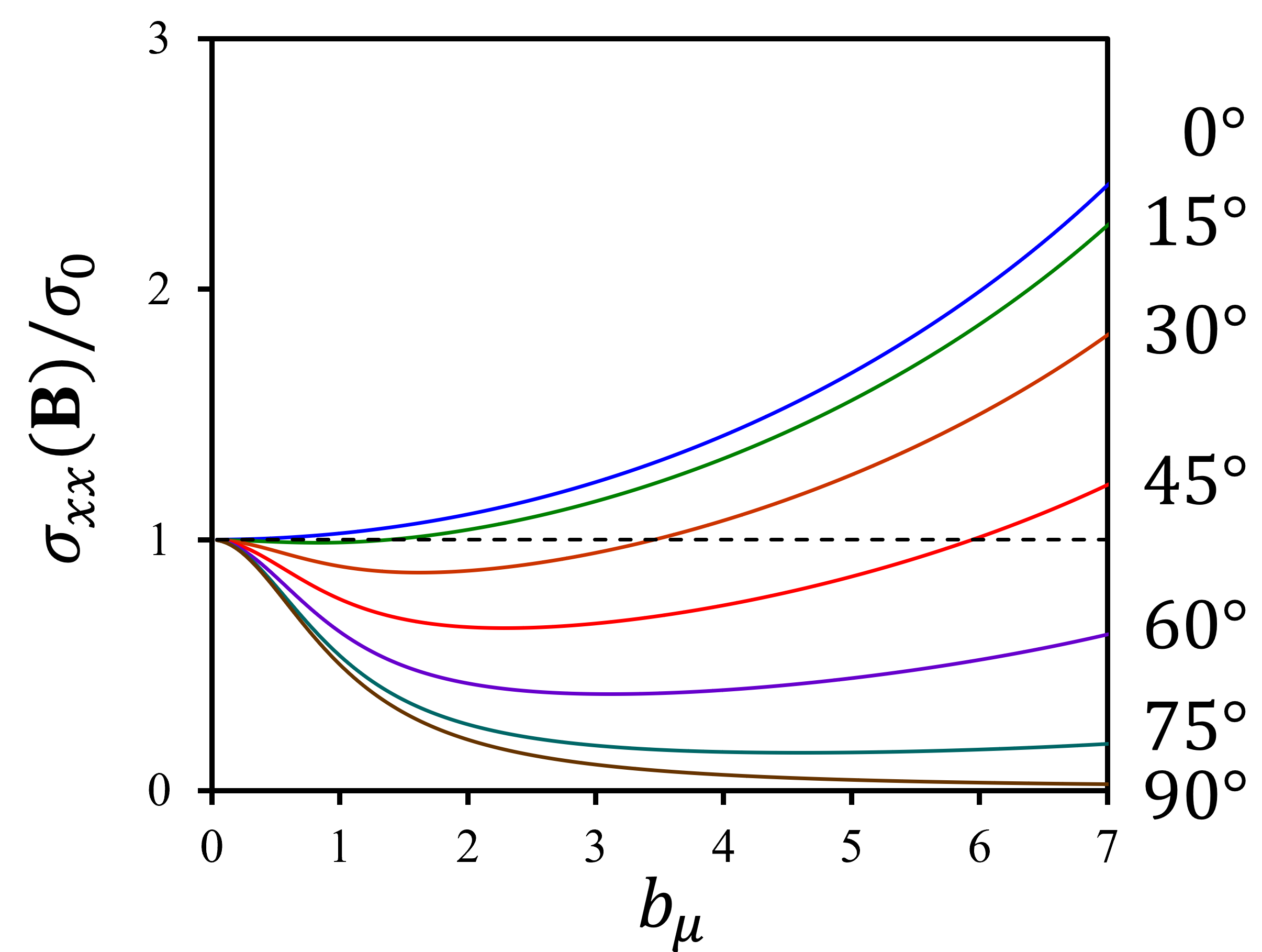
Note that in Eq. (25) is independent of , as comes with a power of two. Thus, the contribution from multiple degenerate Weyl nodes enters as a degeneracy factor when internode scatterings are neglected. Most of previous works for longitudinal magnetoconductivity in WSMs using Boltzmann transport theory reported where is the additional positive magnetoconductivity that scales quadratically in magnetic field KIM2014 ; DAI2017 ; NANDY2017 ; IMRAN2018 . Instead, Eq. (25) shows a non-monotonic behavior of magnetoconductivity in magnetic field due to the competition between the Berry curvature and Lorentz force depending on , as shown in Fig. 2. This result is consistent with the previous calculation for WSMs obtained by expanding the non-equilibrium distribution function in Fourier harmonics IMRAN2018 .
We now come back to the approximation we made: . Note that for weak magnetic fields, we could Taylor expand as
| (26) |
We emphasize that earlier studies of magnetotransport also took the correction into account but incompletely. For instance, Kim et al. KIM2014 only took even terms in Taylor expanded in Eq. (26) which gave rise to an additional positive correction to magnetoconductivity described in Eq. (25). However, numerical calculations of the full longitudinal magnetoconductivity [Eq. (21)] show a reduced value compared to Eq. (25). The reduced magnetoconductivity is due to terms that are odd orders in in Eq. (21) coupling with odd orders in terms in the Taylor expanded in Eq. (26). As a result, the pairs of odd terms in give rise to non-vanishing even terms in which additionally give negative corrections to the magnetoconductivity.
By incorporating first three terms in Eq. (26), we obtain the longitudinal magnetoconductivity in WSMs up to quadratic order in as
See Appendix B.1 for detailed derivations. This result is well matched with the previous work which focused on specific angles between applied electric and magnetic fields IMRAN2018 .
III.2 Planar Hall conductivity
To investigate the planar Hall conductivity in WSMs, we again set the electric and magnetic field orientations as and , respectively. Neglecting terms that would give zero contribution to conductivity, Eq. (II) gives the following form of the planar Hall conductivity assuming (see Appendix B.2):
| (28) |
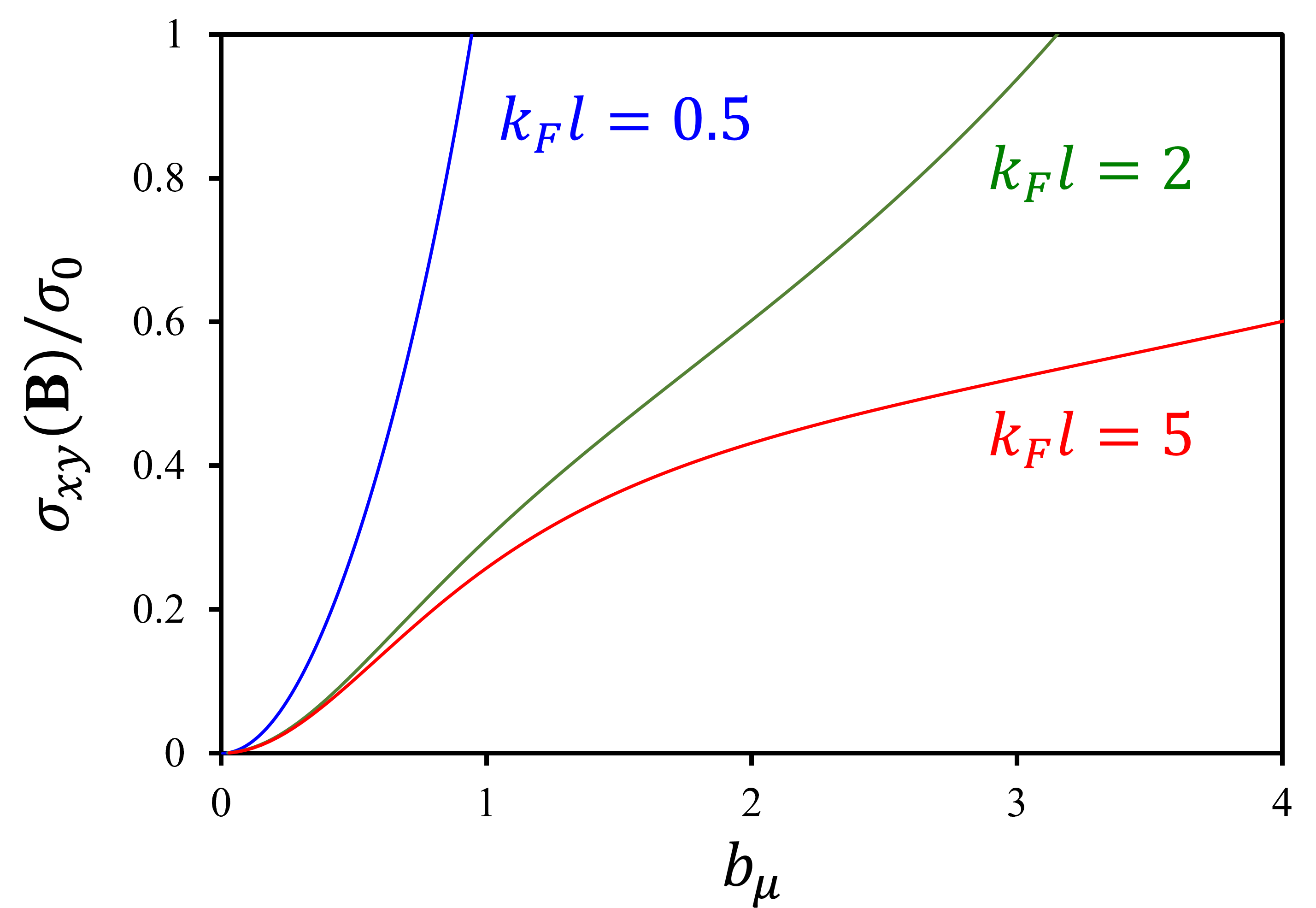
Note that in Eq. (28) is independent of . Equation (28) is the analytic form of the planar Hall conductivity in WSMs for an arbitrary angle of the applied magnetic field . The angle dependence of the planar Hall conductivity is well matched with the previous works BURKOV2017 ; NANDY2017 ; LI2018 ; LIANG2019 ; LIU2019 ; MA2019 ; LI2020 but the field dependence shows an additional contribution from the Lorentz force in addition to a quadratic field dependence due to the Berry curvature. As shown in Fig 3, the planar Hall conductivity shows different dependence at different regimes. For large , the planar Hall conductivity roughly increases with quadratically at low field and saturates at high field. For low regime, the planar Hall conductivity shows dependence with no sign of saturation in a broad range of magnetic field as reported in the previous studies NANDY2017 .
III.3 Hall conductivity
To investigate the Hall conductivity in WSMs, we set the electric and magnetic field orientations as and , respectively. Then Eq. (II) gives the following form of Hall conductivity assuming (see Appendix B 3):
| (30) |
Note that this result is identical to the conventional magnetotransport result. This implies that there is no anomalous velocity effect in the Hall conductivity.
III.4 Conductivity and resistivity tensors
Combining the previous results of magnetoconductivity in WSMs, we obtain the following conductivity tensor under with :
| (32) |
where is the angle between applied electric and magnetic fields. Since the resistivity tensor is the inverse of the conductivity tensor , we obtain in the following form:
| (33) |
where . Note that although both the Lorentz force and the Berry curvature induced terms are present in , the Lorentz force induced terms do not appear in the resistivity where . This result agrees with the previous one reporting that , where () is the resistivity in longitudinal (transverse) magnetic field and is the resistivity anisotropy JAN1957 ; BURKOV2017 . For the conductivity and resistivity tensors including the Taylor expanded , see Appendix B.5.
IV Conclusion
In this work, we presented a closed-form expression for the magnetoconductivity using the semiclassical magnetotransport theory that fully incorporates the Berry curvature and the Lorentz force effects. We then applied this formula to WSMs and obtained analytic expressions for the longitudinal, planar Hall and Hall conductivities in terms of dimensionless parameters and which are normalized magnetic fields associated with the Lorentz force and the Berry curvature, respectively. From these results, we showed a non-monotonic field dependence in the longitudinal and planar Hall conductivities depending on . Furthermore, we clearly demonstrated that although the Lorentz force effect is manifested in the planar Hall conductivity, its contribution vanishes in the planar Hall resistivity.
Acknowledgements.
This work was supported by the National Research Foundation of Korea (NRF) grant funded by the Korea government (MSIT) (Grant No. 2018R1A2B6007837) and Creative-Pioneering Researchers Program through Seoul National University (SNU).References
- (1) H.-J. Kim, K.-S. Kim, J.-F. Wang, M. Sasaki, N. Satoh, A. Ohnishi, M. Kitaura, M. Yang and L. Li, Dirac versus Weyl Fermions in Topological Insulators: Adler-Bell-Jackiw Anomaly in Transport Phenomena, Phys. Rev. Lett. 111, 246603 (2013).
- (2) X. Huang, L. Zhao, Y. Long, P. Wang, D. Chen, Z. Yang, H. Liang, M. Xue, H. Weng, Z. Fang, X. Dai and G. Chen, Observation of the Chiral-Anomaly-Induced Negative Magnetoresistance in 3D Weyl Semimetal TaAs, Phys. Rev. X 5, 031023 (2015).
- (3) J. Xiong, S. Kushwaha, T. Liang, J. Krizan, M. Hirschberger, W. Wang, R. Cava and N. Ong, Evidence for the chiral anomaly in the Dirac semimetal , Science 350, 413 (2015).
- (4) C.-Z. Li, L.-X. Wang, H. Liu, J. Wang, Z.-M. Liao and D.-P. Yu, Giant negative magnetoresistance induced by the chiral anomaly in individual nanowires, Nature Communications 6, 10137 (2015).
- (5) Q. Li, D. E. Kharzeev, C. Zhang, Y. Huang, I. Pletikosić, A. V. Fedorov, R. D. Zhong, J. A. Schneeloch, G. D. Gu and T. Valla, Chiral magnetic effect in , Nature Physics 12, 550 (2016).
- (6) C. Zhang, S.-Y. Xu, I. Belopolski, Z. Yuan, Z. Lin, B. Tong, G. Bian, N. Alidoust, C.-C. Lee, S.-M. Huang, T. Chang, G. Chang, C.-H. Hsu, H. Jeng, M. Neupane, D. Sanchez, H. Zheng, J. Wang, H. Lin, C. Zhang, H.-Z. Lu, S. Shen, T. Neupert, M. Z. Hasan and S. Jia, Signatures of the Adler-Bell-Jackiw chiral anomaly in a Weyl fermion semimetal, Nature Communications 7, 10735 (2016).
- (7) H. Li, H. He, H.-Z. Lu, H. Zhang, H. Liu, R. Ma, Z. Fan, S.-Q. Shen and J. Wang, Negative magnetoresistance in Dirac semimetal , Nature Communications 7, 10301 (2016).
- (8) C. Zhang, E. Zhang, W. Wang, Y. Liu, Z.-G. Chen, S. Lu, S. Liang, J. Cao, X. Yuan, L. Tang, Q. Li, C. Zhou, T. Gu, Y. Wu, J. Zou and F. Xiu, Room-temperature chiral charge pumping in Dirac semimetals, Nature Communications 8, 13741 (2017).
- (9) J. Wang, H. Li, C. Chang, K. He, J. S. Lee, H. Lu, Y. Sun, X. Ma, N. Samarth, S. Shen, Q. Xue, M. Xie and M. Chan, Anomalous anisotropic magnetoresistance in topological insulator films, Nano Research 5, 739 (2012).
- (10) H. T. He, H. C. Liu, B. K. Li, X. Guo, Z. J. Xu, M. H. Xie and J. N. Wang, Disorder-induced linear magnetoresistance in (221) topological insulator films, Applied Physics Letters 103, 031606 (2013).
- (11) L.-X. Wang, Y. Yan, L. Zhang, Z.-M. Liao, H.-C. Wu and D.-P. Yu, Zeeman effect on surface electron transport in topological insulator nanoribbons, Nanoscale 7, 16687 (2015).
- (12) S. Wiedmann, A. Jost, B. Fauqué, J. van Dijk, M. J. Meijer, T. Khouri, S. Pezzini, S. Grauer, S. Schreyeck, C. Brüne, H. Buhmann, L. W. Molenkamp and N. E. Hussey, Anisotropic and strong negative magnetoresistance in the three-dimensional topological insulator , Phys. Rev. B 94, 081302(R) (2016).
- (13) F. Arnold, C. Shekhar, S.-C. Wu, Y. Sun, R. D. dos Reis, N. Kumar, M. Naumann, M. O. Ajeesh, M. Schmidt, A. G. Grushin, J. H. Bardarson, M. Baenitz, D. Sokolov, H. Borrmann, M. Nicklas, C. Felser, E. Hassinger and B. Yan, Negative magnetoresistance without well-defined chirality in the Weyl semimetal TaP, Nature Communications 7, 11615 (2016).
- (14) O. Breunig, Z. Wang, A. A. Taskin, J. Lux, A. Rosch and Y. Ando, Gigantic negative magnetoresistance in the bulk of a disordered topological insulator, Nature Communications 8, 15545 (2017).
- (15) B. A. Assaf, T. Phuphachong, E. Kampert, V. V. Volobuev, P. S. Mandal, J. Sánchez-Barriga, O. Rader, G. Bauer, G. Springholz, L. A. de Vaulchier and Y. Guldner, Negative Longitudinal Magnetoresistance from the Anomalous Landau Level in Topological Materials, Phys. Rev. Lett. 119, 106602 (2017).
- (16) H. Nielsen and M. Ninomiya, The Adler-Bell-Jackiw anomaly and Weyl fermions in a crystal, Physics Letters B 130, 389 (1983).
- (17) D. T. Son and B. Z. Spivak, Chiral anomaly and classical negative magnetoresistance of Weyl metals, Phys. Rev. B 88, 104412 (2013).
- (18) A. Sekine, D. Culcer and A. H. MacDonald, Quantum kinetic theory of the chiral anomaly, Phys. Rev. B 96, 235134 (2017).
- (19) X. Dai, Z. Du and H.-Z. Lu, Negative Magnetoresistance without Chiral Anomaly in Topological Insulators, Phys. Rev. Lett. 119, 166601 (2017).
- (20) K.-S. Kim, H.-J. Kim and M. Sasaki, Boltzmann equation approach to anomalous transport in a Weyl metal, Phys. Rev. B 89, 195137 (2014).
- (21) S. Nandy, G. Sharma, A. Taraphder and S. Tewari, Chiral Anomaly as the Origin of the Planar Hall Effect in Weyl Semimetals, Phys. Rev. Lett. 119, 176804 (2017).
- (22) M. Imran and S. Hershfield, Berry curvature force and Lorentz force comparison in the magnetotransport of Weyl semimetals, Phys. Rev. B 98, 205139 (2018).
- (23) A. Johansson, J. Henk and I. Mertig, Chiral anomaly in type-I Weyl semimetals: Comprehensive analysis within a semiclassical Fermi surface harmonics approach, Phys. Rev. B 99, 075114 (2019).
- (24) J. Suh, S. Park and H. Min, Semiclassical Boltzmann magnetotransport theory in anisotropic systems with a nonvanishing Berry curvature, arXiv:2110.08816 (2021).
- (25) D. Xiao, J. Shi and Q. Niu, Berry Phase Correction to Electron Density of States in Solids, Phys. Rev. Lett. 95, 137204 (2005).
- (26) N. W. Ashcroft and N. D. Mermin, Solid State Physics, Brooks Cole (1976).
- (27) J. M. Ziman, Electrons and phonons: the theory of transport phenomena in solids, International series of monographs on physics, Clarendon Press, Oxford (1960).
- (28) D. Xiao, M.-C. Chang and Q. Niu, Berry phase effects on electronic properties, Rev. Mod. Phys. 82, 1959 (2010).
- (29) R. B. Atencia, Q. Niu and D. Culcer, Semiclassical response of disordered conductors: Extrinsic carrier velocity and spin and field-corrected collision integral, Phys. Rev. Research 4, 013001 (2022).
- (30) A. A. Burkov, Giant planar Hall effect in topological metals, Phys. Rev. B 96, 041110(R) (2017).
- (31) P. Li, C. H. Zhang, J. W. Zhang, Y. Wen and X. X. Zhang, Giant planar Hall effect in the Dirac semimetal , Phys. Rev. B 98, 121108(R) (2018).
- (32) D. D. Liang, Y. J. Wang, W. L. Zhen, J. Yang, S. R. Weng, X. Yan, Y. Y. Han, W. Tong, W. K. Zhu, L. Pi and C. J. Zhang, Origin of planar Hall effect in type-II Weyl semimetal , AIP Advances 9, 055015 (2019).
- (33) Q. Liu, F. Fei, B. Chen, X. Bo, B. Wei, S. Zhang, M. Zhang, F. Xie, M. Naveed, X. Wan, F. Song and B. Wang, Nontopological origin of the planar Hall effect in the type-II Dirac semimetal , Phys. Rev. B 99, 155119 (2019).
- (34) D. Ma, H. Jiang, H. Liu and X. C. Xie, Planar Hall effect in tilted Weyl semimetals, Phys. Rev. B 99, 115121 (2019).
- (35) Z. Li, T. Xiao, R. Zou, J. Li, Y. Zhang, Y. Zeng, M. Zhou, J. Zhang and W. Wu, Planar Hall effect in , Journal of Applied Physics 127, 054306 (2020).
- (36) J.-P. Jan, Galvanomagnetic and Thermomagnetic Effects in Metals, vol. 5 of Solid State Physics, 1–96, Academic Press (1957).
Appendix A Derivation of the nonequilibrium distribution function
Here we go through a detailed derivation of the nonequilibrium distribution function. Let us start with Eq. (12) in the main text:
| (34) |
where is the inverse mass tensor and
| (35) |
To solve in Eq. (34), note that Eq. (34) is given by the following self-consistent form for a vector :
| (36) |
where and are vectors and is a matrix. Then Eq. (36) can be rewritten as
| (37) |
where . Thus, we have
| (38) |
Using the above result Eq. (38), we obtain as the following form:
| (39) |
where is the magnetic field strength tensor. Finally, the nonequilibrium distribution function is given by
| (40) |
The mobility tensor is defined as
| (41) |
which is in general a non-diagonal matrix. For a system with an isotropic energy dispersion in the absence of a magnetic field, the mobility tensor is given by a scalar multiple of an identity matrix. For simplicity, we assume that the mobility tensor is set to a constant . Then, we can rewrite Eq. (34) as
| (42) |
Note that Eq. (42) is given by the following self-consistent form for a vector :
| (43) |
where and are vectors. Then Eq. (43) can be rewritten as
| (44) | |||||
Here, we used and . Thus, we have
| (45) |
Using the result of Eq. (45), we therefore obtain as the following form:
| (46) |
Note that Eq. (39) is reduced to Eq. (46) when the mobility tensor is given by .
Finally, the nonequilibrium distribution function is given by
| (47) |
Appendix B Magnetoconductivity of Weyl semimetals
In this section, we derive the magnetoconductivity of Weyl semimetals including the Taylor expanded . Here we set the magnetic field orientation as .
B.1 Longitudinal magnetoconductivity
Here we go through a detailed derivation of the longitudinal magnetoconductivity. Let us start with Eq. (21) in the main text:
| (48) |
where is a sum of the terms that include th order of described in Eq. (22) in the main text which corresponds to conductivity of respectively. Inserting the Taylor expanded density of states correction
| (49) |
to Eq. (48) and focusing on , yields
| (50) |
where we replaced for zero temperature. Expanding and throwing away terms that will give zero contribution after the momentum integral due to odd order in , we are left with the following angular integral after switching to spherical coordinates then integrating out:
| (51) |
where
| (52) | ||||
Finally, carrying out the angular integral leads to
| (53) |
where is the longitudinal magnetoconductivity in the absence of magnetic field.
Focusing now on , yields
| (54) |
The above whole expression vanishes after the momentum integral, because as . This will lead to a single order in in every term in the integrand therefore result in zero after integration.
Finally, focusing on , yields
| (55) | |||||
Simplifying the product of the Taylor expanded and terms in the square bracket while again, keeping only the non-zero contribution, we are left with the following angular integral after switching to spherical coordinates then integrating out:
| (56) |
where
| (57) | ||||
Finally, carrying out the angular integral leads to
| (58) |
Adding up the s, we have
| (59) |
B.2 Planar Hall conductivity
Here we go through a detailed derivation of the planar Hall conductivity. Starting with Eq. (20) in the main text for , we again express it in powers of while using the definition for . We then obtain,
| (60) |
where
| (61a) | ||||
| (61b) | ||||
| (61c) | ||||
each corresponds to planar Hall conductivity of respectively. Inserting the Taylor expanded density of states correction
| (62) |
to Eq. (60) and focusing on , yields
| (63) | |||||
where we replaced for zero temperature. Expanding and throwing away terms that will give zero contribution after the momentum integral due to odd order in , we are left with the following angular integral after switching to spherical coordinates then integrating out:
| (64) |
where
| (65) | ||||
Finally, carrying out the angular integral leads to
| (66) |
Focusing now on , yields
| (67) |
The above whole expression vanishes after the momentum integral, because as . This will lead to a single order in in every term in the integrand therefore result in zero after integration.
Finally, focusing on , yields
| (68) | |||
Simplifying the product of the Taylor expanded and terms in the square bracket while again, keeping only the non-zero contribution, we are left with the following angular integral after switching to spherical coordinates then integrating out:
| (69) |
where
| (70) | |||||
Finally, carrying out the angular integral leads to
| (71) |
Adding up the s, we have
| (72) |
B.3 Conductivity
Here we go through a detailed derivation of . Starting with Eq. (20) in the main text for , we again express it in powers of while using the definition for . We then obtain
| (73) |
where
| (74a) | ||||
| (74b) | ||||
| (74c) | ||||
each corresponds to Hall conductivity of respectively. Inserting the Taylor expanded density of states correction to Eq. (73) and focusing on , yields
| (75) |
where we replaced for zero temperature. The above whole expression in Eq. (75) vanishes after the momentum integral.
Focusing now on , yields
| (76) |
Expanding and throwing away terms that will give zero contribution after the momentum integral due to odd order in , we are left with the following angular integral after switching to spherical coordinates then integrating out:
| (77) |
where
| (78) |
Finally, carrying out the angular integral leads to
| (79) |
Finally, focusing on , yields
| (80) |
The above expression vanishes after the momentum integral.
B.4 Conductivity
Here we go through a detailed derivation of the . Starting with Eq. (20) in the main text for , we again express it in powers of while using the definition for . We then obtain
| (82) |
where
| (83a) | ||||
| (83b) | ||||
| (83c) | ||||
as . Note that after the momentum integral, will vanish due to odd order in . The only remaining contribution is from which gives
| (84) | ||||
B.5 Conductivity and resistivity tensors
Finally, we have the following conductivity tensor including the Taylor expanded :
The resistivity tensor is then obtained by the inverse of the conductivity tensor as
| (86) |
Note that although both the Lorentz force and the Berry curvature induced terms are present in , the Lorentz force induced terms do not appear in the resistivity where even if we include the Taylor expanded .