Semi-supervised Learning Meets Factorization: Learning to Recommend with Chain Graph Model
Abstract.
Recently latent factor model (LFM) has been drawing much attention in recommender systems due to its good performance and scalability. However, existing LFMs predict missing values in a user-item rating matrix only based on the known ones, and thus the sparsity of the rating matrix always limits their performance. Meanwhile, semi-supervised learning (SSL) provides an effective way to alleviate the label (i.e., rating) sparsity problem by performing label propagation, which is mainly based on the smoothness insight on affinity graphs. However, graph-based SSL suffers serious scalability and graph unreliable problems when directly being applied to do recommendation. In this paper, we propose a novel probabilistic chain graph model (CGM) to marry SSL with LFM. The proposed CGM is a combination of Bayesian network and Markov random field. The Bayesian network is used to model the rating generation and regression procedures, and the Markov random field is used to model the confidence-aware smoothness constraint between the generated ratings. Experimental results show that our proposed CGM significantly outperforms the state-of-the-art approaches in terms of four evaluation metrics, and with a larger performance margin when data sparsity increases.
1. Introduction
As e-commerce platforms and online social networks provide customers and users myriad products and massive information, a recommender system (RS) has become a useful and even indispensable facility for information filtering. In fact, RS is now part of our daily activities, as it has been widely adopted by internet service leaders, such as Amazon, Youtube, and Facebook (Sarwar et al., 2001).
Latent factor model. Among the existing recommendation approaches, latent factor model (LFM) has been drawing much attention due to its good performance and scalability. LFM uses a low dimensional user and item latent factors to represent the characteristics of each user and each item, and uses the product of them to represent the user’s rating on the item. LFM has drawn much attention recently due to its good performance and scalability (Mnih and Salakhutdinov, 2007; Koren, 2008; Takács et al., 2008; Agarwal and Chen, 2009; Rendle, 2010; Wang and Blei, 2011; Purushotham et al., 2012; Kanagal et al., 2013; Xu et al., 2015; Liu et al., 2016; Guo et al., 2016; Beutel et al., 2017). As users have actions (e.g., rate and buy) on some items, LFM aims to predict the users’ unknown actions on other items. The tendency of a user’s action on an item can be indicated by a real-valued number, i.e., rating or label. Thus, the recommendation problem is also known as the unknown ratings prediction problem (Shi et al., 2014). In practice, however, many LFMs have to evaluate very large user and item sets, where the user-item (U-I) matrix is extremely sparse– such data sparsity has always been its main challenge (Su and Khoshgoftaar, 2009).
Semi-supervised learning. SSL uses unlabeled data to either modify or reprioritize hypotheses obtained from labeled data alone, and thus can alleviate the label sparsity problem by adopting the graph information between data (Seeger, 2002). Towards effective SSL, affinity graph-based smoothness approaches have attracted much research interests, which follow the smoothness insight: close nodes on an affinity graph have similar labels. Graph-based SSL is appealing recently because it is easy to implement and gives rise to closed-form solutions (Zhu et al., 2003; Chapelle et al., 2006; Wang et al., 2006; Ding et al., 2007; Wang and King, 2010; Fang et al., 2014). However, graph-based SSL directly predicts the unknown ratings in the original U-I matrix, and thus suffers from the scalability problem.
As a key insight of this paper, we identify the marriage of SSL and LFM. The main insights of SSL (i.e., smoothness) and LFM (i.e., dimensionality reduction) are orthogonal, and they are likely to benefit from each other. However, surprisingly, the synergy between SSL and LFM has not been explored. On one hand, the smoothness idea of SSL, i.e., similar users or items should give or receive similar ratings– across the entire U-I matrix of ratings, known or unknown, can mitigate the data sparsity problem of LFM. On the other hand, the dimensionality reduction idea of LFM can solve the scalability problem of SSL, since the prediction is done in a low rank matrix instead of the original high dimensional matrix.
Challenges of marrying SSL with LFM. However, marrying SSL with LFM to do recommendation is nontrivial. We summarize the main challenges as follows:
Challenge : Disparate unification. SSL predicts unknown ratings through rating propagation on affinity graphs. I.e., SSL captures the correlation dependency between ratings. LFM predicts unknown ratings through learning user and item latent factors by regressing known ratings. I.e., LFM captures the causal dependency between latent factors and ratings. Therefore, we aim to propose a principled framework to unify SSL and LFM so that such different dependency between different variables can be captured.
Challenge : Expensive graph construction. In a RS scenario, each data object is a U-I pair, with a rating as its label, and thus, to adopt SSL for rating prediction in RS, rating smoothness should exist among U-I pairs. Suppose we have I users and J items, building such a U-I pairwise affinity graph needs to compute the similarity between each of U-I pairs, with a time complexity of , and thus, cannot scale to large datasets. Thus, we aim to realize smoothness in a more efficient manner.
Challenge : Unreliable affinity. In a traditional SSL scenario, the affinity graphs are built based on the characteristics of the data itself, e.g., the pixel data of a scanned digit. In contrast, in a RS scenario, the affinity graphs are usually built based on user social relationships or ratings (Wang et al., 2006; Ding et al., 2007; Wang and King, 2010; Purushotham et al., 2012; Ma et al., 2011; Gu et al., 2010; Chen et al., 2014). As a result, the affinity graphs are unreliable due to the sparsity of such user social relationships or ratings (U-I pairs). Thus, we aim to alleviate the unreliable affinity problem in a robust way.
Our proposal: Learning to recommend with CGM. Our proposal is based on the following insights.
Insight : Principled unification. To address Challenge , we propose a novel chain graph model (CGM) to marry SSL with LFM. As far as we know, this is the first attempt in the literature to adopt CGM in RS. A CGM is a combination of Bayesian network and Markov random field, which has the ability to capture different kinds of dependency (i.e., correlation and causal dependency) between different kinds of variables (i.e., latent factors and ratings) (Lauritzen and Richardson, 2002; Bishop, 2006; Mackey, 2007). Thus, CGM is an ideal model to solve Challenge .
Insight : Efficient smoothness. To address Challenge , we develop a novel “joint smoothness” framework to realize SSL on a pair of decomposed user and item affinity graphs. Since a rating is given from a user to an item, smoothness exists in two dimensions, i.e., user and item. We term it joint-smoothness, which enables us to decrease the time complexity to build affinitive graphs to .
Insight : Selective smoothness. To address Challenge , we propose a confidence-aware smoothness approach. Different from the traditional SSL which performs rating propagation (i.e., smoothness constraint) everywhere on the affinity graphs, we choose to perform smoothness selectively. Specifically, we propose a smoothness confidence decay model to control the hops of rating propagation length.
Solutions. First, we propose a novel CGM (Section 4), which is a combination of Bayesian network and Markov random field. Second, we propose a joint-smoothness objective function. Instead of building a U-I pairwise affinity graph, we build two decomposed user and item affinity graphs. Third, we propose a confidence-aware smoothness approach (Section 5.3). This selective smoothness approach not only alleviates the graph unreliable problem in RS scenarios, but also saves huge computation. Finally, we present the model learning method based on coordinate descent (Section 6).
Results. We concretely realize our solutions of marrying SSL with two kinds of popular LFMs, and conduct comprehensive experiments in Section 7. Our experiments are conducted on three popular datasets, with nine state-of-the-art comparison approaches. We use four metrics to evaluate model performance. The experimental results show that our approach significantly outperforms the state-of-the-art methods, especially in data sparsity scenarios.
Contributions. We summarize the main contributions in this paper as follows:
-
•
We propose a novel CGM to marry SSL with LFM for alleviating the data sparsity problem of RS, which we believe is the first attempt in the literature.
-
•
We propose to perform joint-smoothness instead of pairwise smoothness, which has better efficiency.
-
•
We propose a confidence-aware smoothness approach to alleviate the unreliable graph problem in RS scenario. To the best of our knowledge, it is also the first attempt.
-
•
Our model scales linearly with the observed data size, since we adopt dimensionality reduction technique and confidence-aware smoothness approach.
The rest of the paper is organized as follows. In Section 2, we review related work. In Section 3, we describe the popular realizations of SSL and LFM. In Section 4, we propose a novel probabilistic CGM to marry SSL with LFM. In Section 5, we present the confidence-aware joint-smoothness energy function. In Section 6, we present the model learning approach based on gradient descent. In Section 7, we present the experimental results and analysis. Finally, we conclude the paper in Section 8.
2. Related Work
As described in Section 1, we want to marry SSL with LFM by using chain graph model (CGM), in this section, we review literature on SSL, LFM, LFR, and CGM, respectively.
2.1. Semi-supervised learning
SSL uses unlabeled data to either modify or reprioritize hypotheses obtained from labeled data alone (Seeger, 2002). Among the existing SSL techniques, graph-based SSL is the most promising one, which alleviates data sparsity problem by performing label propagation on the affinity graphs, and its main insight is graph-based smoothness (Zhu et al., 2003; Fang et al., 2014). In the literature, several different objective functions are proposed to realize graph-based smoothness, e.g., Harmonic Function (HF) (Zhu et al., 2003) and Green’s Function (GF) (Ding et al., 2007). Take HF for example, it minimizes the rating difference between close nodes and thus achieves smoothness on , which is the same as propagate the known labels to the unknown ones on the affinity graph (Zhu and Ghahramani, 2002). So far, there are several research directly adopting SSL to do rating prediction (Wang et al., 2006; Ding et al., 2007; Wang and King, 2010). However, as described in Section 1, directly adopting them in RS suffers from scalability and unreliable affinity problems.
2.2. Latent factor model.
Generally, existing LFMs can be divided into three types: basic matrix factorization (MF) that only uses U-I rating matrix to do prediction, side information aided MF that uses other side information besides the U-I rating matrix, and latent factor restriction models that consider user/item affinity graphs.
Basic matrix factorization. MF has drawn much attention recently since it was adopted in the Netflix competition (Koren, 2008), and its main insight is the dimensionality reduction technique (Sarwar et al., 2000). The most basic MF model, known as probabilistic matrix factorization (PMF) or single value decomposition (SVD), factorizes a U-I matrix into a low rank user feature matrix and item feature matrix, and then uses their product to predict unknown ratings (Mnih and Salakhutdinov, 2007; Takács et al., 2008; Xu et al., 2015; Hernando et al., 2016; Liu et al., 2016; Beutel et al., 2017; Feng et al., 2017). Other promotions of SVD include SVDB and SVD++, which further consider user/item rating bias and implicit feedback information (Koren, 2008).
Matrix factorization with side information. Generally, side information can be divided into three categories: content information, social information, and other context information, e.g., user attributes. These three kinds of information have been proven efficient to improve recommendation performance (Agarwal and Chen, 2010; Wang and Blei, 2011; McAuley and Leskovec, 2013; Chen et al., 2014; Agarwal and Chen, 2009; Rendle, 2010; Agarwal and Chen, 2010; Jamali and Ester, 2010; Jiang et al., 2014; Guo et al., 2016; Chen et al., 2016a; Chen et al., 2016b; Yan et al., 2017).
First, regression-based latent factor model (RLFM) (Agarwal and Chen, 2009) and factorization machines (Rendle, 2010) were proposed to incorporate context information to improve recommendation performance. However, these context information are not always available and hard to obtain, and thus they are out of the scope of this paper. Second, the integration of factor model and LDA (fLDA) (Agarwal and Chen, 2010) further incorporates item content information into RLFM. Third, Wang et al. propose collaborative topic regression (CTR) (Wang and Blei, 2011), which systematically combines PMF and latent Dirichlet allocation (LDA) (Blei et al., 2003). CTR uses PMF to factorize U-I rating information and uses LDA to mine item content information. It has been proven that CTR outperforms fLDA in a similar setting, since fLDA largely ignores the other users ratings (Wang and Blei, 2011). Later, CTR-SMF (Purushotham et al., 2012) was proposed to factorize not only rating information but also user social information to make a better recommendation.
However, existing LFMs only fit the model by minimizing the difference between the rare known ratings and the predicted ratings, and do not consider rating smoothness nature between similar U-I pairs.
Latent factor restriction. The most similar works to ours are LFRs (Ma et al., 2011; Gu et al., 2010; Chen et al., 2014; Rao et al., 2015). They first use rating or side information to build user or item affinity graphs, and then constrain latent factor smoothness on the graphs. They assume that connected user or item on the affinity graphs should have similar latent factors. We divide the existing LFRs into two types, i.e, user latent factor restriction (ULFR) (Ma et al., 2011; Chen et al., 2014) and user-item latent factor restriction (UILFR) (Gu et al., 2010), which means that only user latent factor and both user and item latent factors are restricted, respectively.
LFR is actually not the smoothness insight as captured in SSL, i.e., rating smoothness. LFR is much stronger than rating smoothness constrain, because LFR leads to rating smoothness, but not the other way around. Take an item affinity graph for example: based on the assumption of LFR, all the ratings of the connected items should be similar, since neighbors have similar latent factors. That is, LFR indicates smoothness exists everywhere on an affinity graph. Our experiments in Section 7 will demonstrate that this overly strong assumption will fail particularly in data sparsity scenarios.
2.3. Chain Graph Models.
CGM is a probabilistic model that combines Bayesian network and Markov random field. Bayesian network is useful to express causal relationships between random variables (Bishop, 2006), and it is popularly used in the existing LFMs (Mnih and Salakhutdinov, 2007; Agarwal and Chen, 2009; Wang and Blei, 2011), which use Bayesian network to express the rating generation procedure. Markov random field is suited to express soft constraints between random variables (Bishop, 2006), and its applications also include recommender systems (Domingos and Richardson, 2001). Chain graph models contain both Bayesian network and Markov random field, and thus can represent a broader class of distributions, and it has been used in applications include image de-noising (Mackey, 2007), while, surprisingly, not in RS so far.
There are existing works try to bridge collaborative filtering and SSL (Cao et al., 2013; Zhang et al., 2014; Yang et al., 2017). For example, Semi-SAD (Cao et al., 2013) tried to combine the idea of collaborative filtering and SSL for shilling attack detection tasks. The semi-supervised co-training (CSEL) framework (Zhang et al., 2014) first proposes two context-aware factorization models by leveraging “more general” sources such as age and gender of a user, or the genres. Then, it builds a semi-supervised learning process by assembling two models generated with the above context-aware model. This method belongs to context-aware recommendation approaches and needs to use contextual information, e.g., user age and item category, which is out-of-the-scope of our paper. Preference and context embedding (PACE) (Yang et al., 2017) aim to bridge collaborative filtering and graph-based SSL to do point-of-interest (POI) recommendation through a neural approach, which is the most relevant and state-of-the art model. Specifically, PACE uses Skipgram (Mikolov et al., 2013) to model graph-based context information as the SSL part, and uses a multi-layer neural network to model user-POI interaction information as the collaborative filtering part.
In this paper, we propose a novel CGM to marry LFM with SSL to do the geneal recommendation tasks, and we also propose a confidence-aware approach to solve the overly strong assumption of LFR. Our work is different from it mainly from the following three aspects: (1) PACE only aims to do POI recommendation, while our model can be applied into most recommendation scenarios; (2) The objective function of PACE is designed for binary ratings (i.e., a rating ), while our model is suitable for any rating scales (i.e., a rating ); (3) PACE assumes the affinity graph is reliable due to its application to POI recommendation where affinity graph can be built using location information. In contrast, as one of the main contributions of our work, we propose a solution for alleviating the graph unreliable problem in many general recommendation situations. We will show the comparison results in experiments: the performance of PACE is limited in the general recommendation scenarios where affinity graph is unreliable.
3. Preliminary
Since both SSL and LFM can be used to alleviate the data sparsity problem of RS, in this section, we will present the popular approaches of both of them.
Problem setting. In RS, each data object, i.e., a U-I pair, is related to two elements, i.e., user and item. The data label, i.e., U-I rating, is generated from a user to an item. Suppose there is a U-I pairwise affinity graph with nodes denote data objects, edges denote the affinitive relationship between nodes, and weights of edges denote the affinitive relation strength between nodes. Let and be the user and item latent feature matrixes, with their column vectors and representing the K-dimensional latent vectors of and respectively.
Semi-supervised learning approaches. Graph-based SSL mainly alleviates the data sparsity problem by realizing the smoothness insight on affinity graphs, i.e., close nodes on an affinity graph should have similar labels (Zhu et al., 2003; Fang et al., 2014). In the literature, several different objective functions are proposed to realize graph-based smoothness, e.g., Harmonic Function (HF) (Zhu et al., 2003) and Green’s Function (GF) (Ding et al., 2007). Take HF for example, its energy function on a pairwise affinity graph is
| (1) |
where and are two nodes on and is the weight between them. controls the global smoothness degree on and a bigger corresponding to a higher rating smoothness degree on . Eq. (1) minimize the rating difference between close nodes and thus achieves smoothness on , which is the same as propagate the known labels to the unknown ones on the affinity graph (Zhu and Ghahramani, 2002).
Latent factor models. As we described in Section 2, two promising kinds of LFMs are the basic MF and side information-aided MF. The basic MF approach uses to capture ’s overall interests in ’s characteristics, that is the predicted rating of on (Mnih and Salakhutdinov, 2007). Its object is to minimize the difference between the observed ratings and the predicted ratings:
| (2) |
where is an indicator function that equals to 1 if rated , 0 otherwise, denotes the Frobenius norm, and and are regularization parameters to avoid overfitting.
The side information-aided MF incorporate other information, e.g., item content and context information, to learn a better prior for user and item latent factors. For example, CTR (Wang and Blei, 2011) additionally includes a topic proportion which learned from item’s content using topic modeling when modeling item latent factor. For its model details, please refer to (Wang and Blei, 2011).
From the above explanation of the existing LFMs, we can see that they only focus on fitting the model by regressing the rare known ratings, and neglect the rating smoothness insight between similar users and items.
4. Proposed Chain Graph Model


| Notation | Meaning |
|---|---|
| label confidence matrix | |
| user prior mean | |
| item prior mean | |
| user prior confidence | |
| item prior confidence | |
| global smoothness degree on user graph | |
| global smoothness degree on item graph | |
| smoothness confidence decay parameter |
In this section, we propose a novel probabilistic CGM to marry SSL with LFM, which is Insight (i.e., principled unification).
4.1. Problem Statement
We first define our recommendation problem. Given a user set and an item set , there are totally ratings, among which only ratings are known, and our recommendation task is to predict the unknown ratings, with the size of .
As described in Section 1, SSL and LFM are popularly used to solve the above recommendation problem, however, they have their own merits and disadvantages. Since we want to marry SSL with LFM, we first use a toy example to illustrate how SSL and LFM make recommendation separately. Let be the U-I rating matrix, with each element denoting the rating that gives to . Let be the predicted U-I rating matrix, with its real-valued rating denoting the predicted rating of on . Figure 1 (a) shows a U-I rating matrix example, where we have two users ( and ), two items ( and ), and two known U-I rating pairs ( and ). Our mission is to predict the two unknown U-I pairs ( and ).
Graph-based SSL makes recommendation mainly based on the smoothness idea on affinity graphs. Since each data object in RS is a U-I rating pair, to make recommendation, SSL first needs to build a U-I pairwise affinity graph, and then propagates the known U-I rating pairs to the unknown ones. Let be a U-I pairwise affinity graph with nodes denoting data objects, edges denoting the affinitive relationship between nodes, and weight matrix between edges denoting the affinitive relation strength between nodes. Figure 1 (b) shows how to adopt SSL to do recommendation, where the affinity graph is shown in dash lines, and we do not show the edge weight for conciseness. Predictions will be made by propagating and to and . That is, the purpose of SSL is rating smoothness on affinity graphs, and SSL captures the mutual dependency between ratings.
LFM makes recommendation mainly based on the dimensionality reduction idea. Let and be the user and item latent feature matrixes, with their column vectors and representing the K-dimensional latent vectors of and respectively. Figure 1 (c) shows how to use LFM to do recommendation. LFM predicts the unknown ratings by learning user and item latent factors through regressing on the known ones. In this example, LFM predicts and by learning , , , and through regressing on and . That is, the purpose of LFM is rating regression, and LFM captures the causal dependency between latent factors and ratings.
Although LFM and SSL have different purpose, they both are actually used to capture different dependency between different variables. To marry LFM with SSL, we need a model so that such different dependency between different variables can be captured.
4.2. Regression and Smoothness Based Chain Graph Model
We identify probabilistic CGM, a powerful tool for representing the relationship between variables, to be ideal for marrying LFM with SSL. CGM is a combination of Bayesian network and Markov random field (Koller and Friedman, 2009; McCarter and Kim, 2014). First, Bayesian network, i.e, directed probability graphical model, is commonly used to model the causal dependency between variables. Second, Markov random field, i.e., undirected probability graphical model, is used to model the mutual dependency between variables.
To marry LFM with SSL, the proposed CGM should serve for two goals, as we described in the above example: (1) Rating regression. The predicted rating should be close to the observed rating; (2) Rating smoothness. The predicted ratings should be smooth between close U-I pairs. Thus, we call our model Regression and Smoothness-based Chain Graph Model (RSCGM).
Our proposed RSCGM combines Bayesian network and Markov random field. Figure 1 (d) shows an our proposed CGM example, where we use the directed graph (shows with solid arrows) to model rating generation and known rating regression procedures, and use the undirected graph (shows with dash lines) to model the rating smoothness constrain on an affinity graph. RSCGM is a three layer probabilistic graphical model. The first layer is the latent factor layer, and its nodes are latent variables, i.e., and . The second layer is the prediction layer, and its nodes are the predicted ratings, i.e., . The third layer is the observation layer, and its nodes are the observed data, i.e., . From the latent factor layer to the prediction layer, it is a Bayesian network which denotes the rating generation procedure; I.e., we use as the prediction of a U-I pair. The prediction layer is a Markov random field which denotes the prediction smoothness constrain. From the prediction layer to the observation layer, it is another Bayesian network which denotes the rating regression objective, i.e., the predicted rating should be close to the observed rating.
Joint distribution over all the variables. We first give the joint distribution over all the variables in all the three layers. The Markov property of chain graph model (Lauritzen and Richardson, 2002), i.e., conditional independence relations between variables, indicates that the probability of a node on a CGM only depends on its directed neighbors. Thus, we factorize the joint distribution over all the variables as:
| (3) |
We then derive the conditional probabilities of variables in each layer.
Latent factor layer. Our model starts with latent factors which is also the start of the Bayesian network. We place Gaussian priors on user latent factor:
| (4) |
where is a -dimensional identity matrix, and is the probability density function of the Gaussian distribution with mean and variance . Note that is the user prior mean matrix with each column denoting the mean of each user latent factor. can be obtained from additional information. For example, (Jamali and Ester, 2010) takes the average preference of a user’s friends as the mean of his prior. Similarly, we place another Gaussian prior on item factor:
| (5) |
where is the item prior mean matrix with each column denoting the mean of each item latent factor, which can also be obtained from additional information. For example, CTR (Wang and Blei, 2011) takes the topic allocation learned from the content information of an item as the mean of its prior.
Prediction layer. The prediction comes from the latent factor layer, and has smoothness constrain between themselves. As a result, the probability of depends on two independent parts: (1) variables from the first layer, i.e., and ; (2) affinitive neighbors on user and item affinity graphs. The first part corresponds to the directed graph that comes from the latent factor layer to the prediction layer in Figure 1. The second part corresponds to the undirected graph in the second layer of Figure 1. Based on the Markov property of chain graph model (Lauritzen and Richardson, 2002), we have
| (6) |
where is a normalizer that makes sure the probability equals to 1.
In Eq. (6), we define the first term with denoting the Dirac delta function (Dirac, 1958), and the property of Dirac delta function indicates that integrating out is equivalent to replacing with , which is the rating generation procedure. The second term is probability that constrains rating smoothness with denoting the rating smoothness energy function on affinity graphs, i.e., the confidence-aware joint-smoothness objective function that we will present in Section 5.
Observation layer. Each node in the observation layer is an observed rating of an prediction from the prediction layer, and it corresponds to the rating regression part from the prediction layer to the observation layer in Figure 1. As a result, the probability of is conditional on in the prediction layer. We adopt a Gaussian prior here, the same as the existing LFM (Mnih and Salakhutdinov, 2007):
| (7) |
where is a label confidence matrix with each element denoting the label confidence for each U-I pair, and more details refer to (Wang and Blei, 2011).
Posterior distribution over latent factors. Finally, we use maximum a posteriori (MAP) probability to learn the best and . Based on Eq. (3), Eq. (4), Eq. (5), Eq. (6), and Eq. (7), we have the following posterior distribution over user and item latent factors by using Bayes’ theorem,
| (8) |
We will present how to learn the MAP distribution over the user and item latent factors in Section 6.
5. Realizing Smoothness
In this section, we present the confidence-aware joint-smoothness energy function, which will enable us to obtain shown in Eq. (6).
5.1. From Pairwise to Joint Smoothness
Pairwise smoothness has severe scalability problem. As Section 1 mentioned, building such an affinity graph requires for users and items, i.e., Challenge . To solve it, we propose an efficient way to perform smoothness.
In RS, each data object connects two elements, i.e., user and item. Thus, rating smoothness implies smoothness exists on two elements, i.e., user and item, and we term it “joint smoothness”. We try to find the relationship between pairwise and joint smoothness. Figure 2 shows a derivation example from pairwise to joint smoothness, where we have three users and two items, and we simply use to denote pair. For any two pairs on , e.g., and ( or ), based on HF (Zhu et al., 2003), pairwise objective energy function in Eq. (1) can be further divided into the following three terms based on different and combinations:
| (9) |
where
| (10) |


First, we remove the diagonal edges from the pairwise graph, i.e., remove from Eq. (9). Figure 2(b) shows the result after we remove the diagonal edges from Figure 2(a). We use to denote the difference between and , i.e., , to denote the difference between and , i.e., , and to denote the difference between and , i.e., . We know that the difference between and has a upper bound of , since , i.e, . In other words, the rating smoothness between and and the rating smoothness between and will result in the rating smoothness between and . Thus, we can still achieve diagonal rating smoothness after we remove diagonal edges.
Second, we compute the edge affinity weight. The U-I pairwise affinity is determined by both user and item affinity, and thus, we take pairwise affinity as a function of user affinity and item affinity. Specifically, we assume , where is a function of the similarity between and , is a function of the similarity between and , and is a function of the similarity between and . We also assume for all the users and for all the items, which means that the similarity between a node itself is 1. For any , since holds, i.e., the weight between any and pairs is the same regardless of , we can represent all such weights with one, i.e., which is the similarity between and . Similarly, we use to represent the similarity between and .
Next, since and , we can merge nodes, as shown in Figure 2(c). Specifically, we merge nodes for the into one node which has labels, and we merge nodes for all the into one node which has labels, as shown in Figures 2(d) and 2(e). That is, we decompose the pairwise graph into user and item joint graphs, and decrease the time complexity to build joint affinity graphs to by computing the similarity between users and items separately. Thus, and change to:
| (11) |
| (12) |
Finally, to achieve joint smoothness, we need to leverage the effect of user and item rating smoothness. To do this, we use two parameters, i.e., and , to control the global smoothness degree on and . Combining Eq. (11) and Eq. (12), we define joint smoothness objective as:
| (13) |
where a bigger corresponds to a higher user rating smoothness degree on and a bigger a higher item rating smoothness degree on . We will perform experiments to compare pairwise and joint smoothness in Section 7.4.
5.2. User and Item affinity Graphs
We now explain how to build user and item affinity graphs.
User affinity graph. A user affinity graph should capture affinitive relationships between users, so that the ratings of close users will be similar, as we define below:
Definition 1: A user affinity graph is an undirected weighted graph , where (1) is the node set; that is, each node is a user with labels, corresponding to the ratings each user gives to all them items; (2) is the edge set, with denoting the weight of edge ; that is, is the relationship strength between nodes and , which is symmetric, i.e., .
We suggest to build user affinity graph using whatever information that is available to capture the affinitive relationships between users, e.g., ratings and user social relationships. For example, user social relationships also indicate users’ common interests, and thus can be taken as the user affinity graph.
Item affinity graph. Similarly, an item affinity graph should capture affinitive relationships between items, so that the ratings of close items will be similar, as defined as below:
Definition 2: An item affinity graph is an undirected weighted graph , where (1) is the node set; that is, each node is an item with labels, corresponding to the ratings it receives from all the users; (2) is the edge set, with denoting the weight between of edge ; that is, is the relationship strength between nodes and , which is symmetric, i.e., .
One can also build item affinity graph using whatever information that is available to capture the affinitive relationships between items, e.g., ratings and item content information. Frequently, cosine similarity, Jaccard’s coefficient (JC), and Pearson correlation coefficient (PCC) are used to measure rating similarity between items (Ma et al., 2011).
The quality of the affinity graphs, e.g., the reliability and density of the graph, significantly affects the recommendation result. The joint affinity graphs we build are unreliable, since we use rare existing information. Thus, we propose a confidence-aware approach to realize smoothness on them. We will further study the effects the affinity graph on recommendation performance during experiments.
5.3. Confidence-aware Joint-smoothness
We finally present a confidence-aware approach to realize smoothness, which solves Challenge (i.e., unreliable affinity).
Confidence-aware user rating smoothness. User rating smoothness on constrains that close users on have similar ratings on items. This is consistent with the reality: e.g., Alice is wondering which movie to watch, and she finds her close friends gave high ratings to “The Dark Knight”, and she is likely to watch “The Dark Knight”.
The built affinity graphs are unreliable, and thus full smoothness, i.e., assuming smoothness exists everywhere, will be an overly strong assumption. We identify to solve this by using selective smoothness approach. As described in Section 2, rating smoothness can be viewed as propagating known ratings to unknown ones. Since the user affinity graph is unreliable, intuitively, smoothness confidence will decrease with the rating propagation length.
To achieve confidence-aware user rating smoothness, we propose a confidence decay parameter, i.e., , to control rating propagation length. Figure 3 shows a user affinity graph, where we have three users and two items. Although we use only one edge to express the similarity for and pairs, there is actually a smoothness confidence between them. From Figure 3, we can see how the rating smoothness confidence decreases with propagation length. For example, the smoothness confidence between and should be bigger than that between and , since the label of , i.e., , will first be propagated to and then to .
In general, suppose we have two users ( and ) and an item (), we define the smoothness confidence between and pairs as:
| (14) |
where is the confidence decay parameter that ranges in [0, 1], and with and denoting the distances from and to a user whose rating on is given, respectively.
The proposed confidence-aware smoothness approach, on one hand, alleviates the overly strong assumption of fully smoothness, and, on the other hand, reduces computation. For and on and any , given smoothness confidence in Eq. (14) and following Eq. (11), we define confidence-aware user rating smoothness energy function as:
| (15) |

Confidence-aware item rating smoothness. Similarly, item rating smoothness on restricts that close items have similar ratings. This is also consistent with reality: e.g., Alice has watched movie “The Dark Knight” and loves it so much. She then finds “Batman Begins” is a similar movie, and she will probably likes “Batman Begins” as well.
Similar to user rating smoothness, for and on and any , following Eq. (12), we define confidence-aware item rating smoothness energy function as,
| (16) |
where has the similar meaning to Eq. (14).
Following Eq. (13), combining Equations (15) & (16), we define confidence-aware joint smoothness energy function as:
| (17) |
Having will enable us to obtain shown in Eq. (6).
6. Model Parameter Learning
Based on Equations (4), (5), (6), (7), and (17), the posterior distribution over the user and item latent factors in Eq. (8) becomes
| (18) |
Maximizing the log of the posterior probability is equivalent to minimizing the following objective function:
| (19) |
where we replace with . We minimize Eq. (19) by performing coordinate descent approach, that is, we fix the hyper-parameters, and iteratively optimize the user and item latent factors and .
Specifically, we take the gradient of with respect to and , set it to zero and get,
| (20) |
| (21) |
We summarize the learning of RSCGM in Algorithm 1. After the optimal and are learned, they can be used to make predictions through .
Computation Analysis. We now analysis the time complexity of our model inference. From Eq. (19), we can see that the time complexity of realizing our model is , where is the size of observed data, and are the average number of edges we need to do rating smoothness (propagation) in and .
Due to the data sparsity problem, the best value of is usually very small (about 0.5 in our experiments), which indicates that the known ratings will only be propagated to their close U-I pairs. With a big , the smoothness degree will decay by which will be so small that can be neglected. Due to the data sparsity problem, the average number of neighbors on and are usually very small, which indicates that and . Besides, since , our algorithm scales linearly with the observed data size .
7. Experiments
In this section, we present the comprehensive experiments that aimto answer four key questions: (1) How well does our approach handle the data sparsity problem when comparing with the state-of-the-art approaches? (2) What is the performance difference between pairwise smoothness and joint smoothness? (3) How do user/item affinity graph and model parameters , , and affect our model performance? (4) What is the time complexity of our approach?
7.1. RSCGM Realizations
Our proposed RSCGM is a general model to marry SSL with LFM. As described in Section 2, there are mainly two kinds of LFMs in existing work. Thus, we apply RSCGM into both of them, i.e., a basic MF (BMF) (Mnih and Salakhutdinov, 2007) and a content-based MF (CMF) (Wang and Blei, 2011). BMF assumes zero mean Gaussian on both user and item latent factors, i.e., , while CMF assumes zero mean Gaussian on user latent factor and an item topic allocation mean Gaussian on item latent factor, i.e., and , where is the topic allocation learned from item content information using topic modeling technique (Wang and Blei, 2011).
7.2. Experiment Setting
Datasets. To study how RSCGM behaves under the BMF scenario, we use Movielens-10M dataset (MovieLens) (Harper and Konstan, 2016) and the classic Netflix dataset (Bennett and Lanning, 2007). Both datasets are popular and famous, and the ratings of which are integers that rage from 0 to 5. To study how RSCGM behaves under the CMF scenario, we use hetrec2011-delicious-2k dataset (Delicious) and dataset hetrec2011-lastfm-2k (Lastfm) (Cantador et al., 2011). These datasets, as described in Table 2, have been popularly used (Purushotham et al., 2012). For MovieLens and Netflix, we compute the PCC similarity between users and items to build user and item affinity graphs. For Delicious and Lastfm, we consider the rating of a user on an item as ‘1’ if this user has bookmarked (or listened) this item, ‘0’ otherwise, and we take the tags of each item as its content information. We use user social information to build user affinity graph, and compute the JC similarity between items to build item affinity graph.
| Dataset | users | items | tags | user social relations | U-I ratings | rating density |
|---|---|---|---|---|---|---|
| MovieLens | 71,567 | 10,681 | – | – | 10,000,054 | 1.31% |
| Netflix | 480,189 | 17,770 | – | – | 100,480,507 | 1.18% |
| Delicious | 1,867 | 69,226 | 53,388 | 15,328 | 104,799 | 0.08% |
| Lastfm | 1,892 | 17,632 | 11,946 | 25,434 | 92,834 | 0.28% |
Baseline methods. For BMF scenario, we compare RSCGM with the following state-of-the-art methods:
-
•
ICF (Sarwar et al., 2001) is an item-based collaborative filtering approach.
- •
-
•
BMF (Mnih and Salakhutdinov, 2007) is a classic MF approach.
-
•
BMF-ULFR (Ma et al., 2011) adds user latent factor restriction (ULFR) on BMF.
-
•
BMF-UILFR (Gu et al., 2010) adds both user and item latent factor restriction (UILFR) on a weighted nonnegative MF approach. To make a fair comparison, we replace the weighted nonnegative MF approach with BMF.
For CMF scenario, we compare RSCGM with the following state-of-the-art methods:
-
•
CMF (Wang and Blei, 2011) is a popular content information aided MF approach.
-
•
CMF-SMF (Purushotham et al., 2012) adds user social factorization in CMF.
-
•
CMF-ULFR (Chen et al., 2014) adds ULFR on CMF.
-
•
CMF-UILFR (Gu et al., 2010) adds UILFR on a weighted nonnegative MF approach. To make a fair comparison, we also replace the weighted nonnegative MF approach with CMF.
- •
Evaluation metrics. Since ratings range from ‘1’ to ‘5’ on MovieLens, we use Mean Absolute Error (MAE) and Root Mean Square Error (RMSE) to evaluate prediction performance (Ma et al., 2011; Chen et al., 2014):
| (22) |
| (23) |
where is the number of predictions in the test dataset .
Since ratings range in {‘0’, ‘1’} on Delicious and Lastfm, we use Precision and Recall to evaluate prediction performance (Wang and Blei, 2011; Purushotham et al., 2012). For each user, precision and recall are defined as follows:
where M is the returned items. We compute the average of all the users’ precision and recall in the test dataset as the final result.
Parameter setting: Before comparison, we first use fivefold cross validation to find the best values of and , and then we set accordingly for other models. For parameter in CMF-SMF, in BMF-ULFR and CMF-ULFR, and in BMF-UILFR and CMF-UILFR, and and in our model, we find their best values in [, , , , , , ]. We also search the best value of in our model in [0, 1]. All the experiments are done on a PC by using OpenMP222http://openmp.org/ to perform parallel computing.
7.3. Comparison Results and Analysis
We compare our proposed model, i.e., RSCGM, with the state-of-the-art approaches on all the four dataset to prove the effectiveness of our approach. Our experiments are divided into two parts: comparison with the existing BMF-based models and comaprision with the existing CMF-based models.
7.3.1. Comparison with BMF-based models
First, we report the experiments of comparing RSCGM and the existing BMF models conducted on MovieLens and Netflix datasets. Since our key insight of this paper is to use the idea of SSL to alleviate the data sparsity problem of LFM, we focus on evaluating each model’s performance under different data sparsity scenerios. We use two strategies to generate datasets with different spasity: (1) rating sample, that is, we randomly sample some ratings and remove them from the original MovieLens and Netflix datasets, and (2) user sample, that is, we remove the users whose ratings are bigger than a certain threshold. Through rating sample strategy, we get several sub-datasets with diffferent sparsity, i.e., MovieLens-x%, which means we randomly remove x% of the ratings from the original dataset. Similarly, through user sample strategy, we get several sub-datasets with diffferent sparsity, i.e., MovieLens-y, which means we remove the users whose rating numbers are bigger than y. Rating sample and user sample strategies can also be used together, and MovieLens-y-x% means we first use user sample strategy to remove the users whose rating numbers are bigger than y and then randomly remove x% of the ratings from the rest dataset.
| Datasets | MovieLens | MovieLens-70% | MovieLens-80% | MovieLens-85% | MovieLens-90% | MovieLens-95% | ||||||
| Sparsity | 1.31% | 0.39% | 0.26% | 1.97% | 0.14% | 0.07% | ||||||
| Metrics | MAE | RMSE | MAE | RMSE | MAE | RMSE | MAE | RMSE | MAE | RMSE | MAE | RMSE |
| SSL | 0.7848 | 1.1315 | 0.7987 | 1.1434 | 0.8100 | 1.1548 | 0.8273 | 1.1788 | 0.8606 | 1.2173 | 1.0407 | 1.4385 |
| ICF | 0.7318 | 0.9494 | 0.7966 | 1.0319 | 0.8211 | 1.0619 | 0.8398 | 1.0889 | 0.8613 | 1.1136 | 0.9087 | 1.1681 |
| BMF | 0.6356 | 0.8290 | 0.6780 | 0.8831 | 0.6934 | 0.9022 | 0.7072 | 0.9244 | 0.7446 | 0.9681 | 0.8254 | 1.0785 |
| BMF-ULFR | 0.6351 | 0.8277 | 0.6767 | 0.8805 | 0.6933 | 0.9014 | 0.7020 | 0.9178 | 0.7446 | 0.9679 | 0.8023 | 1.0376 |
| BMF-UILFR | 0.6351 | 0.8277 | 0.6752 | 0.8762 | 0.6916 | 0.8948 | 0.7000 | 0.9098 | 0.7415 | 0.9586 | 0.7958 | 1.0317 |
| RSCGM | 0.6352 | 0.8240 | 0.6702 | 0.8678 | 0.6818 | 0.8810 | 0.6889 | 0.8928 | 0.7268 | 0.9385 | 0.7899 | 1.0166 |
| improv. vs. BMF | 0.07% | 0.5% | 1.15% | 1.74% | 1.67% | 2.35% | 2.58% | 3.42% | 2.39% | 3.05% | 4.31% | 5.73% |
| Datasets | Sparsity | Metrics | SSL | ICF | BMF | BMF-ULFR | BMF-UILFR | RSCGM | improv. vs. BMF |
| MovieLens-100 | 0.44% | MAE | 0.8362 | 0.8192 | 0.7409 | 0.7250 | 0.7232 | 0.7172 | 3.20% |
| RMSE | 1.2115 | 1.0680 | 0.9677 | 0.9435 | 0.9422 | 0.9331 | 3.58% | ||
| MovieLens-75 | 0.37% | MAE | 0.8706 | 0.8316 | 0.7715 | 0.7531 | 0.7481 | 0.7442 | 3.53% |
| RMSE | 1.2606 | 1.0850 | 1.0070 | 0.9844 | 0.9737 | 0.9555 | 5.11% | ||
| MovieLens-50 | 0.30% | MAE | 0.8958 | 0.8616 | 0.8105 | 0.7781 | 0.7724 | 0.7649 | 5.62% |
| RMSE | 1.2895 | 1.1244 | 1.0543 | 1.0118 | 1.0029 | 0.9858 | 6.50% |
| Datasets | Sparsity | Metrics | SSL | ICF | BMF | BMF-ULFR | BMF-UILFR | RSCGM | improv. vs. BMF |
| Netflix-200-70% | 0.14% | MAE | 0.8846 | 0.8639 | 0.7573 | 0.7569 | 0.7532 | 0.7477 | 1.27% |
| RMSE | 1.2968 | 1.1147 | 0.9856 | 0.9827 | 0.9710 | 0.9534 | 3.26% | ||
| Netflix-200-80% | 0.09% | MAE | 0.9187 | 0.8879 | 0.7738 | 0.7708 | 0.7673 | 0.7625 | 1.45% |
| RMSE | 1.3418 | 1.1463 | 1.0058 | 0.9975 | 0.9814 | 0.9691 | 3.65% | ||
| Netflix-200-90% | 0.05% | MAE | 1.0264 | 0.9131 | 0.7943 | 0.7939 | 0.7882 | 0.7750 | 2.43% |
| RMSE | 1.4781 | 1.1758 | 1.0347 | 1.0118 | 1.0009 | 0.9842 | 4.89% |
During our experiments, we use five-fold cross validation method. Table 3 shows the MAE and RMSE comparison result on different rating sample MovieLens datasets. Table 4 shows the MAE and RMSE comparison result on different user sample MovieLens datasets. Table 5 shows the MAE and RMSE comparison result on different user and rating sample MovieLens datasets. From them, we have the following observations:
-
•
The latent factor models significantly outperforms SSL and ICF, due to its dimensionality reduction technique.
-
•
With the increase of the data sparsity degree, the performance of all the models decrease. This is the standard data sparsity problem.
-
•
our approach always achieves the best performance. Besides, no matter which kind of sample strategy we use, either rating sample, user sample, or both user and rating sample, there is an obvious trend: the sparser the dataset is, the bigger improvement of our model against the comparison methods. Take the experimental results on different sampled Netflix datasets for example, the RMSE improvement of our approach over BMF are 3.26%, 3.65%, and 4.89% on Netflix-200-70%, Netflix-200-80%, and Netflix-200-90% respectively.
7.3.2. Comparison with CMF-based models


Next, we report the experiments of comparing RSCGM and the existing CMF models conducted on Delicious and Lastfm datasets. Note that the original Delicious dataset is already quite sparse (0.08%) and Lastfm dataset is relative dense. We use rating sample strategy on Lastfm to generate datasets with different sparsity degress, and we get Lastfm20 and Lastfm50 whose sparsity are 0.22% and 0.14%, respectively. Figure 4 shows the Recall performance on Delicious and Lastfm, and we omit the Precision performance since it is similar to Recall. Figure 5 shows the Precision performance for each model on different sparsity of datasets, and here we omit the Recall performance since it is similar to Precision. From it, we get:
-
•
With the increase of the data sparsity degree, the performance of all the models decrease. This is the standard data sparsity problem.
-
•
With the increase of the latent factor dimensionality , the performances of all the models increase, since a bigger will represent a better latent factor. However, as we will analysis later, it comes with price of higher model training time.
-
•
CMF-SMF and CMF-ULFR slightly outperform CMF due to the additional user social information. Meanwhile, CMF-UILFR adopts additional user and item graph information and achieves better performance. Moreover, PACE behaves as a constant runner-up due to its deeper network to handle rating and affinity graph information. However, PACE uses graph embedding technique to learn user/item latent factors, which assumes graphs are strongly reliable. Thus, the performance of PACE is limited in graph unreliable situations, although it enjoys great performance in POI recommendation scenario.
-
•
With the increase of the data sparsity degree, CMF, CMF-SMF, and LFRs (CMF-ULFR and CMF-UILFR) tend to have more similar performance. This is because LFRs’ performance are limited due to their overly strong assumption that connected users or items tend to share similar latent factors. This overly strong assumption of LFR fails particularly when affinity graphs are unreliable in the data sparsity scenario.
-
•
Our model (RSCGM) significantly outperforms PACE and consistently achieves the best performance among all the approaches on all the datasets. Because the marriage of SSL and LFM and the realization of the confidence-aware joint-smoothness.
7.4. Compare Pairwise and Joint Smoothness
We then study the runtime performance (including graph build time and model inference time) and prediction performance between pairwise and joint smoothness. As analysied in Section 5.1, building a pairwise affinity graph is quite time-consuming, i.e., Challenge . To compare pairwise and joint smoothness, we use hetrec2011-movielens-2k dataset (MovieLens2K) (Cantador et al., 2011), which is a relative small dataset. MovieLens2K contains 2,113 users, 10,197 items, and 855,598 U-I rating pairs. We then use different smoothness objective function, i.e., the pairwise smoothness shown in Eq. (1) and the joint smoothness shown in Eq. (13), in our proposed model. We term joint smoothness “joint” here for simplification. We also use two kinds of approaches to build the pairwise affinity graph, i.e., (1) “pairwise1”: , and (2) “pairwise2”: . We finally compare their runtime and prediction differences on MovieLens2K. The results are shown in Table 6, where we set . As we analyzed in Section 5.1, the runtime of joint smoothness is significantly shorter than pairwise smoothness. Besides, the prediction performance of joint smoothness also outperforms pairwise smoothness. This is because joint smoothness uses two parameters ( and ) to control the global smoothness degree on and separately. In contrast, pairwise smoothness uses only one parameter () to control the global smoothness degree on . Thus, joint smoothness can leverage smoothness degree more delicately on affinity graphs.
| Metric | MAE | RMSE | runtime (seconds) |
|---|---|---|---|
| pairwise1 | 0.7071 | 0.9170 | 337 |
| pairwise2 | 0.6889 | 0.8916 | 157 |
| joint | 0.6185 | 0.8188 | 5 |
7.5. Effect of Affinity Graph and Model Parameters

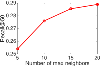
As we described in Section 5.2, the affinigy graph significantly affects the final performance, and therefore, we first study the effect of user/item affinity graphs on our model performance. The user/item affinity graphs aim to capture the affinitive relationships between users/items. The more precise the built user/item affinity graphs capture all the latent affinitive relationships between users/items, the better our model learns user/item latent factors. We change the user/item affinity graphs by varying the number of max neighbors. Figure 6 shows the effect of the number of max neighbors of the affinity graphs on our model performance, where we set . From it, we observe that with the increase of the number of max neighbors of the affinity graphs, our model performance first increases and then becomes stable. The results indicate that the quality of the affinity graphs are important for our model performance.


We then study the effect of the smoothness degree parameters, i.e., and , on our model performance. By doing this, we set , , which means that we only propagate the known ratings to their direct U-I pairs. Figure 7 shows the effect of and on RSCGM, where we set . We can see that RSCGM achieves the best Precision and Recall performance when on Delicious. The results indicate that smoothness on both user and item affinity graphs contribute to model performance, which proves the effectiveness of our joint-smoothness idea.
We finally study the effect of the smoothness confidence decay parameter, i.e., , on our model performance. By doing this, we set and to the best values obtained above. Figure 8 shows the effect of on RSCGM. From it, we can see that, with the increase of , the performance first increases, and then decreases after a certain threshold. The explanation is: (1) when is small, the smoothness confidence will be too small to propagate ratings. That is, known ratings will only be propagated to short path neighbors and this may cause information loss; (2) On the contrary, with a big , known ratings will be propagated to their long path neighbors, and this may cause data noise due to the unreliable affinity graphs.
7.6. Computation Time
We run our model on a PC with 2.33 GHz Intel(R) Xeon(R) CPU and 8Gb RAM. Figure 9 shows the wall-clock running time per iteration of our proposed model with different size of training data on the Lastfm. The same as we analyzed in Section 6, the runtime does increase linearly with the observed data size. Besides, further observation shows that, the bigger is, the bigger the runtime increase rate is. This is because the runtime can be seen as a linear function of the observed data size, and its slope is . With a relative stable value of , the bigger is, the bigger the increase slope is.


8. Conclusion
In this paper, we have proposed a probabilistic chain graph models to marry SSL with LFM to improve recommendation performance by alleviating the data sparsity problem. The proposed CGM is a combination of Bayesian network and Markov random field. We use the dimensionality reduction idea of LFMs in the Bayesian network, and use the smoothness idea of SSL in Markov random field. We have proposed to perform joint smoothness instead of pairwise smoothness to save affinity graph build time. We also have proposed a confidence-aware approach to realize joint-smoothness to address the affinity unreliable problem in RS. Our proposed approach realized the ideas of both SSL and LFM, and addresses the challenges of adopting SSL in RS, and thus possesses the merits of both LFM and SSL. We have conducted experiments on four popular real world datasets, and the experimental results showed that our approach significantly outperforms the state-of-the-art recommendation approaches, especially in data sparsity scenarios.
References
- (1)
- Agarwal and Chen (2009) Deepak Agarwal and Bee-Chung Chen. 2009. Regression-based latent factor models. In Proceedings of the 15th ACM SIGKDD International Conference on Knowledge Discovery and Data Mining. 19–28.
- Agarwal and Chen (2010) Deepak Agarwal and Bee-Chung Chen. 2010. fLDA: matrix factorization through latent dirichlet allocation. In Proceedings of the Third ACM International Conference on Web Search and Data Mining. 91–100.
- Bennett and Lanning (2007) James Bennett and Stan Lanning. 2007. The netflix prize. In Proceedings of KDD Cup and Workshop 2007 Aug 12, Vol. 2007. 35.
- Beutel et al. (2017) Alex Beutel, Ed H Chi, Zhiyuan Cheng, Hubert Pham, and John Anderson. 2017. Beyond Globally Optimal: Focused Learning for Improved Recommendations. In Proceedings of the 26th International Conference on World Wide Web. International World Wide Web Conferences Steering Committee, 203–212.
- Bishop (2006) Christopher M Bishop. 2006. Pattern recognition and machine learning.
- Blei et al. (2003) David M Blei, Andrew Y Ng, and Michael I Jordan. 2003. Latent dirichlet allocation. Journal of Machine Learning Research 3 (2003), 993–1022.
- Cantador et al. (2011) Ivan Cantador, Peter Brusilovsky, and Tsvi Kuflik. 2011. Second workshop on information heterogeneity and fusion in recommender systems (HetRec2011).. In In Proceedings of the 5th ACM conference on Recommender Systems. 387–388.
- Cao et al. (2013) Jie Cao, Zhiang Wu, Bo Mao, and Yanchun Zhang. 2013. Shilling attack detection utilizing semi-supervised learning method for collaborative recommender system. World Wide Web 16, 5-6 (2013), 729–748.
- Chapelle et al. (2006) Olivier Chapelle, Bernhard Schölkopf, Alexander Zien, et al. 2006. Semi-supervised learning. MIT press Cambridge.
- Chen et al. (2016a) Chaochao Chen, Xiaolin Zheng, Yan Wang, Fuxing Hong, Deren Chen, et al. 2016a. Capturing Semantic Correlation for Item Recommendation in Tagging Systems.. In AAAI. 108–114.
- Chen et al. (2014) Chaochao Chen, Xiaolin Zheng, Yan Wang, Fuxing Hong, and Zhen Lin. 2014. Context-aware Collaborative Topic Regression with Social Matrix Factorization for Recommender Systems. In Proceedings of the Twenty-Eighth AAAI Conference on Artificial Intelligence. 9–15.
- Chen et al. (2016b) Chaochao Chen, Xiaolin Zheng, Mengying Zhu, and Litao Xiao. 2016b. Recommender System with Composite Social Trust Networks. International Journal of Web Services Research (IJWSR) 13, 2 (2016), 56–73.
- Ding et al. (2007) Chris Ding, Horst D Simon, Rong Jin, and Tao Li. 2007. A learning framework using Green’s function and kernel regularization with application to recommender system. In Proceedings of the 13th ACM SIGKDD International Conference on Knowledge Discovery and Data Mining. 260–269.
- Dirac (1958) Paul Dirac. 1958. The principles of quantum mechanics. Oxford university press.
- Domingos and Richardson (2001) Pedro Domingos and Matt Richardson. 2001. Mining the network value of customers. In Proceedings of the 7th ACM SIGKDD International Conference on Knowledge Discovery and Data Mining. 57–66.
- Fang et al. (2014) Yuan Fang, Kevin Chen-Chuan Chang, and Hady Wirawan Lauw. 2014. Graph-based Semi-supervised Learning: Realizing Pointwise Smoothness Probabilistically. In Proceedings of the 31st International Conference on Machine Learning.
- Feng et al. (2017) Shanshan Feng, Jian Cao, Jie Wang, and Shiyou Qian. 2017. Recommendations Based on Comprehensively Exploiting the Latent Factors Hidden in Items’ Ratings and Content. ACM Transactions on Knowledge Discovery from Data (TKDD) 11, 3 (2017), 35.
- Gu et al. (2010) Quanquan Gu, Jie Zhou, and Chris HQ Ding. 2010. Collaborative Filtering: Weighted Nonnegative Matrix Factorization Incorporating User and Item Graphs. In Proceedings of the Tenth SIAM Conference on Data Mining. 199–210.
- Guo et al. (2016) Guibing Guo, Jie Zhang, and Neil Yorke-Smith. 2016. A Novel Recommendation Model Regularized with User Trust and Item Ratings. IEEE Transactions on Knowledge and Data Engineering 28, 7 (2016), 1607–1620.
- Harper and Konstan (2016) F Maxwell Harper and Joseph A Konstan. 2016. The movielens datasets: History and context. ACM Transactions on Interactive Intelligent Systems (TIIS) 5, 4 (2016), 19.
- Hernando et al. (2016) Antonio Hernando, Jesús Bobadilla, and Fernando Ortega. 2016. A non negative matrix factorization for collaborative filtering recommender systems based on a Bayesian probabilistic model. Knowledge-Based Systems 97 (2016), 188–202.
- Jamali and Ester (2010) Mohsen Jamali and Martin Ester. 2010. A matrix factorization technique with trust propagation for recommendation in social networks. In Proceedings of the Fourth ACM Conference on Recommender Systems. 135–142.
- Jiang et al. (2014) Meng Jiang, Peng Cui, Fei Wang, Wenwu Zhu, and Shiqiang Yang. 2014. Scalable recommendation with social contextual information. IEEE Transactions on Knowledge and Data Engineering 26, 11 (2014), 2789–2802.
- Kanagal et al. (2013) Bhargav Kanagal, Arif Ahmed, Shishir Pandey, Vanja Josifovski, Lluis Garcia-Pueyo, and Jiaxin Yuan. 2013. Focused matrix factorization for audience selection in display advertising. In Proceedings of the IEEE 29th International Conference on Data Engineering (ICDE). 386–397.
- Koller and Friedman (2009) Daphne Koller and Nir Friedman. 2009. Probabilistic Graphical Models - Principles and Techniques. MIT Press. 161–168 pages.
- Koren (2008) Yehuda Koren. 2008. Factorization meets the neighborhood: a multifaceted collaborative filtering model. In Proceedings of the 14th ACM SIGKDD International Conference on Knowledge Discovery and Data Mining. 426–434.
- Lauritzen and Richardson (2002) Steffen L Lauritzen and Thomas S Richardson. 2002. Chain graph models and their causal interpretations. Journal of the Royal Statistical Society: Series B (Statistical Methodology) 64, 3 (2002), 321–348.
- Liu et al. (2016) Xinyue Liu, Charu Aggarwal, Yu-Feng Li, Xiangnan Kong, Xinyuan Sun, and Saket Sathe. 2016. Kernelized matrix factorization for collaborative filtering. In SIAM Conference on Data Mining. 399–416.
- Ma et al. (2011) Hao Ma, Dengyong Zhou, Chao Liu, Michael R Lyu, and Irwin King. 2011. Recommender systems with social regularization. In Proceedings of the Fourth ACM International Conference on Web Search and Data Mining. 287–296.
- Mackey (2007) Lester Mackey. 2007. Latent Dirichlet Markov Random Fields for Semi-supervised Image Segmentation and Object Recognition. Technical Report. Citeseer.
- McAuley and Leskovec (2013) Julian McAuley and Jure Leskovec. 2013. Hidden factors and hidden topics: understanding rating dimensions with review text. In Proceedings of the 7th ACM Conference on Recommender Systems. 165–172.
- McCarter and Kim (2014) Calvin McCarter and Seyoung Kim. 2014. On Sparse Gaussian Chain Graph Models. In Advances in Neural Information Processing Systems (NIPS 2014). 3212–3220.
- Mikolov et al. (2013) Tomas Mikolov, Ilya Sutskever, Kai Chen, Greg S Corrado, and Jeff Dean. 2013. Distributed representations of words and phrases and their compositionality. In Advances in neural information processing systems. 3111–3119.
- Mnih and Salakhutdinov (2007) Andriy Mnih and Ruslan Salakhutdinov. 2007. Probabilistic matrix factorization. In Advances in Neural Information Processing Systems (NIPS 2007). 1257–1264.
- Purushotham et al. (2012) Sanjay Purushotham, Yan Liu, and C-C Jay Kuo. 2012. Collaborative Topic Regression with Social Matrix Factorization for Recommendation Systems. Proceedings of the 29th International Conference on Machine Learning (ICML 2012) (2012).
- Rao et al. (2015) Nikhil Rao, Hsiang-Fu Yu, Pradeep K Ravikumar, and Inderjit S Dhillon. 2015. Collaborative filtering with graph information: Consistency and scalable methods. In Advances in Neural Information Processing Systems. 2107–2115.
- Rendle (2010) Steffen Rendle. 2010. Factorization machines. In Proceedings of the 2010 IEEE International Conference on Data Mining. 995–1000.
- Sarwar et al. (2000) Badrul Sarwar, George Karypis, Joseph Konstan, and John Riedl. 2000. Application of dimensionality reduction in recommender system-a case study. Technical Report. DTIC Document.
- Sarwar et al. (2001) Badrul Sarwar, George Karypis, Joseph Konstan, and John Riedl. 2001. Item-based collaborative filtering recommendation algorithms. In Proceedings of the 10th International Conference on World Wide Web. 285–295.
- Seeger (2002) Matthias Seeger. 2002. Learning with labeled and unlabeled data. Technical Report. The University of Edinburgh.
- Shi et al. (2014) Yue Shi, Martha Larson, and Alan Hanjalic. 2014. Collaborative filtering beyond the user-item matrix: A survey of the state of the art and future challenges. ACM Computing Surveys (CSUR) 47, 1 (2014), 3.
- Su and Khoshgoftaar (2009) Xiaoyuan Su and Taghi M Khoshgoftaar. 2009. A survey of collaborative filtering techniques. Advances in artificial intelligence 2009 (2009), 4.
- Takács et al. (2008) Gábor Takács, István Pilászy, Bottyán Németh, and Domonkos Tikk. 2008. Investigation of various matrix factorization methods for large recommender systems. In 2008 IEEE International Conference on Data Mining Workshops. IEEE, 553–562.
- Wang and Blei (2011) Chong Wang and David M Blei. 2011. Collaborative topic modeling for recommending scientific articles. In Proceedings of the 17th ACM SIGKDD International Conference on Knowledge Discovery and Data Mining. 448–456.
- Wang and King (2010) Dingyan Wang and Irwin King. 2010. An Enhanced Semi-supervised Recommendation Model Based on Green’s Function. In International Conference on Neural Information Processing. 397–404.
- Wang et al. (2006) Fei Wang, Sheng Ma, Liuzhong Yang, and Tao Li. 2006. Recommendation on item graphs. In Proceedings of the Sixth International Conference on Data Mining (ICDM’06). 1119–1123.
- Xu et al. (2015) Jingwei Xu, Yuan Yao, Hanghang Tong, Xianping Tao, and Jian Lu. 2015. Ice-breaking: Mitigating cold-start recommendation problem by rating comparison. In Proceedings of the 24th International Conference on Artificial Intelligence. AAAI Press, 3981–3987.
- Yan et al. (2017) Surong Yan, Kwei-Jay Lin, Xiaolin Zheng, Wenyu Zhang, and Xiaoqing Feng. 2017. An Approach for Building Efficient and Accurate Social Recommender Systems using Individual Relationship Networks. IEEE Transactions on Knowledge and Data Engineering (2017).
- Yang et al. (2017) Carl Yang, Lanxiao Bai, Chao Zhang, Quan Yuan, and Jiawei Han. 2017. Bridging Collaborative Filtering and Semi-Supervised Learning: A Neural Approach for POI Recommendation. In Proceedings of the 23rd ACM SIGKDD International Conference on Knowledge Discovery and Data Mining. ACM, 1245–1254.
- Zhang et al. (2014) Mi Zhang, Jie Tang, Xuchen Zhang, and Xiangyang Xue. 2014. Addressing cold start in recommender systems: A semi-supervised co-training algorithm. In Proceedings of the 37th international ACM SIGIR conference on Research & development in information retrieval. ACM, 73–82.
- Zhu and Ghahramani (2002) Xiaojin Zhu and Zoubin Ghahramani. 2002. Learning from labeled and unlabeled data with label propagation. Technical Report. Citeseer.
- Zhu et al. (2003) Xiaojin Zhu, Zoubin Ghahramani, John Lafferty, et al. 2003. Semi-supervised learning using gaussian fields and harmonic functions. In Proceedings of the Twentieth International Conference on Machine Learning (ICML-2003). 912–919.