Semi-supervised Dense Keypoints
Using Unlabeled Multiview Images
Abstract
This paper presents a new end-to-end semi-supervised framework to learn a dense keypoint detector using unlabeled multiview images. A key challenge lies in finding the exact correspondences between the dense keypoints in multiple views since the inverse of the keypoint mapping can be neither analytically derived nor differentiated. This limits applying existing multiview supervision approaches used to learn sparse keypoints that rely on the exact correspondences. To address this challenge, we derive a new probabilistic epipolar constraint that encodes the two desired properties. (1) Soft correspondence: we define a matchability, which measures a likelihood of a point matching to the other image’s corresponding point, thus relaxing the requirement of the exact correspondences. (2) Geometric consistency: every point in the continuous correspondence fields must satisfy the multiview consistency collectively. We formulate a probabilistic epipolar constraint using a weighted average of epipolar errors through the matchability thereby generalizing the point-to-point geometric error to the field-to-field geometric error. This generalization facilitates learning a geometrically coherent dense keypoint detection model by utilizing a large number of unlabeled multiview images. Additionally, to prevent degenerative cases, we employ a distillation-based regularization by using a pretrained model. Finally, we design a new neural network architecture, made of twin networks, that effectively minimizes the probabilistic epipolar errors of all possible correspondences between two view images by building affinity matrices. Our method shows superior performance compared to existing methods, including non-differentiable bootstrapping in terms of keypoint accuracy, multiview consistency, and 3D reconstruction accuracy.
1 Introduction
The spatial arrangement of keypoints of dynamic organisms characterizes their complex pose, providing a computational representation of the way they behave. Recently, computer vision models offer fine grained behavioral modeling through dense keypoints that establish an injective mapping from the image coordinates to the continuous body surface of humans [8] and chimpanzees [36]. These models predict the continuous keypoint field from an image, supervised by a set of densely annotated keypoints, which shows remarkable performance on real-world imagery and brings out a number of applications including 3D mesh reconstruction [55, 54, 35, 51, 7, 21], texture/style transfer [26, 37], and geometry learning [14, 1]. Nonetheless, attaining such densely annotated data is labor intensive, and more importantly, the quality of the annotations is fundamentally bounded by the visual ambiguity of keypoints, e.g., points on textureless shirt. This visual ambiguity leads to a suboptimal model when applying it to out-of-sample distributions. In this paper, we present a new semi-supervised method to learn a dense keypoint detection model from the unlabeled multiview images via the epipolar constraint as shown in Figure 1.

Our main conjecture is that the dense keypoint model is optimal only if it is geometrically consistent across views. That is, every pair of corresponding keypoints, independently predicted by two views, must satisfy the epipolar constraint [9]. However, enforcing the epipolar constraint to learn a dense keypoint model is challenging because (1) the ground truth 3D model is unknown and thus the projections of the 3D model cannot be used as the ground truth dense keypoints; (2) the predicted dense keypoints are inaccurate and continuous over the body surface, and therefore, existing multiview supervision approaches [52, 38, 46] for sparse keypoints are not applicable. In these previous methods, the epipolar constraint was enforced between two keypoints (or features) of which semantic meaning was explicitly defined by a finite set of joints (e.g., elbow channel in a network); and (3) establishing correspondences across views requires knowing an inverse mapping from the body surface to the image that can be neither analytically derived nor differentiable. These challenges limit the performance of previous work [22] that relies on iterative offline bootstrapping, which is not end-to-end trainable, or requires additional parameters to learn for 3D reconstruction111An analogous insight has been used for fundamental matrix, directly computed from correspondences that does not require additional variables for 3D reconstruction..
We tackle these challenges through a probabilistic epipolar constraint by incorporating an uncertainty in correspondences. This new constraint encodes the two desired properties. (1) Soft correspondence: given a keypoint in one image, we define matchability—the likelihood of correspondence for all predicted keypoints in another image based on the distance in the canonical body surface coordinate (e.g., texture coordinate). This allows evaluating geometric consistency in the form of a weighted average of epipolar errors over continuous body surface coordinates, eliminating the requirement of exact correspondences. (2) Geometric consistency: we generalize symmetric Sampson distance [9] for all possible pairs of keypoints from two views to enforce the epipolar constraint, collectively. With these properties, we derive a new differentiable multiview consistency measure that is label-agnostic, allowing us to utilize a large number of the unlabeled multiview images without explicit 3D reconstruction.
We design an end-to-end trainable twin network architecture that takes a pair of images as an input and outputs geometrically consistent dense keypoint fields. This network design builds the affinity maps between two keypoint fields based on the matchability and epipolar errors, which facilitates measuring the probabilistic epipolar errors for all possible correspondences. In addition, inspired by knowledge distillation, we use a pretrained model to regularize network learning, which can prevent degenerate cases. Our method shows superior performance compared to existing methods, including non-differentiable bootstrapping [22] in terms of keypoint accuracy, multiview consistency, and 3D reconstruction accuracy.
Our contributions include: (1) a novel formulation of probabilistic epipolar constraint that can be used to enforce multiview consistency on continuous dense keypoint fields in a differentiable way; (2) a new design of the neural network that enable to precisely measure the probabilistic epipolar error, which allows utilizing a large number of the unlabeled multiview images; (3) a distillation-based regularization to prevent degenerate model learning; (4) strong performance on real-world multiview image data, including Human3.6M [11], Ski-Pose [40], and OpenMonkeyPose [3], outperforming existing methods including non-differentiable dense keypoint learning [22].
Broader Impact Statement The ability to understand animals’ individual and social behaviors is of central importance to multiple disciplines such as biology, neuroscience, and behavioral science. Measuring their behaviors has been extremely challenge due to limited annotated data. This approach offers a way to address this challenge with a limited number of annotated data, which will lead to a scalable behavioral analysis. The negative societal impact of this work is minimum.
2 Related Work
Our framework aims at training a dense keypoint field estimation model via multiview supervision. We briefly review the related works.
Dense Keypoint Field Estimation Finding dense correspondence fields between two images is a challenging problem in computer vision. 3D measurements (e.g., depth and pointcloud) can provide a strong geometric cues which enable matching of deformable shapes [43, 29, 49]. Similarly, in 2D, visual and geometric cues have been used to find the dense correspondence fields in an unsupervised learning [57, 6, 4, 45, 44]. Notably, for special foreground targets such as humans, the dense matching problem can be cast as finding a dense keypoint field that maps pixel coordinates to a canonical body surface coordinates [24] (e.g., DensePose [8]). These works were built upon a large amount of data labeled by crowd-workers and generalized to learn the correspondence fields for face [2] and chimpanzees [36]. Key limitations of these approaches are the inaccuracy of labeling and requirement of large labeled data. We address these limitations by formulating multiview supervision that can enforce geometric consistency, which allows utilizing a large amount of unlabeled multiview images.
Multiview Feature Learning Epipolar geometry can be used to learn a visual representation by transferring visual information from one image to another via epipolar lines or 3D reconstruction. For instance, a fusion layer can be learned to fuse feature maps across views [30]. Such fusion models can be factored into shape and camera components to reduce the number of learnable parameters and improve generalizability [50]. Given the camera calibration, a light fusion module can be learned to directly fuse deep features [10] or heatmaps [56] from other view along corresponding epipolar line. Several works combine multiview image features to form 3D features [13, 47] or view-invariant feature in 2D [32].
Multiview Supervision Synchronized multiview images [11, 15, 53] possess a unique geometric property: images are visually similar yet geometrically distinctive, provided by stereo parallax. Such property offers a new opportunity to learn a geometrically coherent representation without labels. Bootstrapping by 3D reconstruction [22] can be used to learn a keypoint detector supervised by the projection of the 3D reconstruction to enforce cross-view consistency. MONET [52] enables an end-to-end learning by eliminating the necessity of 3D reconstruction and directly minimizing epipolar error. Learning keypoints can be combined with 3D pose estimation [34, 12] by enforcing predicting the same pose in all views while using a few labeled examples with 3D or 2D pose annotations to prevent degeneration. One can alleviate the need for large amounts of annotations by matching the predicted 3D pose with the triangulated pose [19]. Several works further learn a latent representation encoding 3D geometry from images [5, 25] or 2D pose [33, 41] by enforcing consistent embedding, texture [28], and view synthesis [46] across views. Unlike these approaches designed for sparse keypoints where the geometric consistency is applied on finite points, we study geometric consistency on continuous dense keypoint fields. Capture Dense [22] is the closest work to ours, which uses bootstrapping through 3D reconstruction of human mesh model [16]. However, due to the non-differentiable nature of bootstrapping, it is not end-to-end trainable. A temporal consistency has been also used for self-supervise the dense keypoint detector [27].
3 Method
We present a novel method to learn a dense keypoint detector by using unlabeled multiview images. We formulate the epipolar constraint for continuous correspondence fields, which allows us to enforce geometric consistency between views.
3.1 Dense Epipolar Geometry
Given a pair of corresponding images from two different views, a pair of corresponding points , are related by a fundamental matrix given the calibrated cameras, i.e. , where is the fundamental matrix, and is a homogeneous representation of . The measure of geometric consistency between the two images can be written as [9]:
| (1) |
where is the entry of . This measures epipolar error that is the Euclidean distance between and the epipolar line .
Consider an injective dense keypoint mapping that maps a pixel coordinate to a canonical 2D body surface coordinate, i.e., where is the set of the foreground pixels in the image , and is the 2D coordinate in the body surface as shown in Figure 2. This dense keypoint mapping can be learned from annotations, e.g., DensePose [8] for humans where it maps to the texture coordinate of 3D human body surfaces. This mapping is incomplete because there exists missing correspondences in an image due to occlusion. One can find a correspondence between the two images through , i.e., where and the two view images. However, is an injective mapping where the analytic inverse does not exist in general.
Given a point in the image , one can measure the expectation of geometric error by a nearest neighbor search on the body surface space:
| (2) |
where is the expectation of geometric error at . The expectation of the geometric error measures the epipolar error over all possible matches in the other view image, i.e., .
There are two limitations in the nearest neighbor search: (1) The correspondences are not exact, leading to a biased estimate of the geometric error expectation. (2) The argmin operation is not differentiable, which cannot be used to learn a dense keypoint detector in an end-to-end fashion.

Instead, we address these limitations by making use of a soft correspondence, or matchability—a likelihood of a point being matched to another point as shown in Figure 2:
| (3) |
where is the probability of matching between and :
| (4) |
is the domain of the canonical coordinates, is the standard deviation that controls the smoothness of matching, e.g., when , it approximates the nearest neighbor search.
We use the matchability to form a probabilistic epipolar error:
| (5) |
where is the epipolar error between x and x’ weighted by the matchability.
The error expectation of can be computed by marginalizing over all :
| (6) |
That is, the expectation of the geometric error of measures a weighted average of epipolar errors for all possible correspondences. The higher matchability, the more contribution to the error expectation. Unlike Equation (2), Equation (6) does not include the non-differentiable argmin operation. Further, it takes into account all possible pairs of correspondences between two images, which eliminates the bias introduced by the nearest neighbor search.
Given the error expectations over the dense keypoint field, we derive a symmetric dense epipolar error that measures geometric consistency between two images:
| (7) |
where is a visibility indicator:
| (8) |
and are the numbers of foreground pixels visible in and , respectively. is a correspondence tolerance defined in the canonical surface coordinate.
In fact, this dense epipolar error is a generalization of Sampson distance [9] that defines epipolar error between explicit point correspondences (point-to-point). We generalize it to model probabilistic correspondence between two set of points (field-to-field).
Existing approaches such as bootstrapping [22] establish the matching through 3D reconstruction of mesh and enforce the geometric error in an alternating fashion due to the non-differentiability of matching. Our differentiable formulation allows learning the dense keypoint detector in an end-to-end manner, which is flexible and shows superior performance.
3.2 Multiview Semi-supervised Learning
We learn the dense keypoint detector by minimizing the following error:
| (9) |
where is the labeled data loss, is the multiview geometric consistency loss, is the regularization loss, and is the multiview photometric consistency loss. , , and are the weights to control their relative importance.
Supervised Loss We learn the dense keypoint detector from the labeled dataset by minimizing the following error:
| (10) |
where is the ground truth canonical surface coordinates for dense keypoints, is the ground truth canonical surface coordinate at .
Multiview Geometric Consistency Loss We learn the dense keypoint detector from the unlabeled multiview dataset by minimizing dense epipolar error over image pairs:
| (11) |
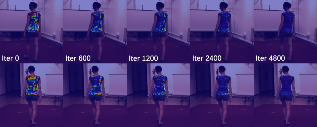
where is the dense epipolar error between two corresponding images and , defined in Equation (7). This loss progressively minimizes the dense epipolar error between image pair as learning the dense keypoint detection model as shown in Figure 3.
Distillation Based Regularization Loss Enforcing multiview consistency alone can lead to degenerate cases. For instance, consider a linear transformation in the body surface, e.g., where is a similarity transformation. Any that satisfies the following condition can be equivalent dense keypoint detector:
| (12) |
This indicates that there exist an infinite number of dense keypoint detectors that satisfy the epipolar geometry. To alleviate this geometric ambiguity, we use a distillation-based regularization using a pretrained model. Let be a dense keypoint detector pretrained by the labeled data. We prevent the learned detector from deviating too much from the pretrained detector for the unlabeled data:
| (13) |
where is the loss for the distillation-based regularization, minimizing the difference from the pretrained model.
Multiview Photometric Consistency Loss We leverage photometric consistency across views. Assuming ambient light, pixels across views corresponding to the same 3D point in space should have the same RGB value. Similar to dense epipolar error , we define dense photometric error as:
| (14) |
where is the expectation of photometric error of similar to , i.e. where .
Then we compute multiview photometric consistency loss as:
| (15) |
3.3 Network Design
We design a new network architecture composed of twin networks to learn the dense keypoint detector by enforcing multiview consistency over dense keypoint fields as shown in Figure 4. Each network is made of a fully convolutional network that outputs the dense keypoint field per body part.
Given two dense keypoint fields, we compute the probabilistic epipolar error by constructing two affinity matrices: matchability matrix and epipolar matrix, where is the cardinality of the range of foreground pixels. These two matrices are defined by:
| (16) |
where is the entry of the matrix . and are the and foreground pixels from the images and , respectively. We also compute the visibility maps and .
We design a new operation to measure the dense epipolar error in Equation (7):
| (17) |
where is the -dimensional vector of which entries are all one. is the element-wise multiplication of matrices. Note that dense epipolar error can be computed following the same operations.

4 Experiments
We perform experiments on human and monkey targets as two example applications to evaluate the effectiveness of our proposed semi-supervised learning pipeline.
4.1 Implementation Details
We use HRNet [42] as the backbone network followed by four head networks made up of convolutional layers to predict foreground mask, body part index, and UV coordinates on the canonical body surface, respectively. Each network takes as an input a 224224 image and outputs 15-channel (for foreground mask head only) or 25-channel 5656 feature maps [8].
We train the network in two stages. In the first stage, we train an initial model using the labeled data by the labeled data loss . Specifically, for the human dense keypoints, we use 48K human instances in DensePose-COCO [8] training set to train the initial model. For the monkey dense keypoints, we directly use the pretrained model for chimpanzees [36] as the initial model since we do not have an access to the labeled data. In the second stage, we train our model on unlabeled multiview data leveraging all losses. The initial model is used for two purposes: (1) the pre-trained model with weights fixed for distillation-based regularization and (2) the initial model to be refined via multiview supervision.
4.2 Evaluation Datasets
Human3.6M [11] is a large-scale indoor multiview dataset captured by 4 cameras for 3D human pose estimation. It contains 3.6 millions of images captured from 7 subjects performing 15 different daily activities, e.g. Walking, Greeting, and Discussion. Following common protocols, we use subject S1, S5, S6, S7 and S8 for training, and reserve subject S9 and S11 for testing. Following [55] and [54], we leverage SMPL [24] parameters generated by HMR [17] via applying MoSh [23] to the sparse 3D MoCap marker data to recover ground truth 3D human meshes. We further perform Procrustes analysis [39] to align them with ground truth 3D poses in global coordinate system and then render ground truth IUV maps using PyTorch3D [31]. Since it is the only multiview human dataset that we have access to ground truth 3D mesh / IUV maps, we use this dataset to perform comprehensive experiment and studies.
3DPW [48] is an in-the-wild dataset made of single view images with accurate 3D human pose and shape annotations. We use the test split of this dataset for dense keypoint accuracy evaluations (3D metrics do not apply). Ground truth IUV maps are rendered from 3D pose and shape annotations by leveraging the provided camera parameters.
Ski-Pose PTZ-Camera Dataset [40] is a multiview dataset capturing competitive skiers performing giant slalom runs. 6 synchronized and calibrated pant-tile-zoom-cameras (PTZ) cameras are used to track a single skier at a time. The global locations of the cameras were measured by a tachymeter theodolite. It contains 8.5K training images and 1.7K testing images. We use this dataset to evaluate generalization towards in-the-wild multiview settings. We use its standard train/test split to train and evaluation our model. We select 6 adjacent view pairs to form training samples.
OpenMonkeyPose [3] is a large landmark dataset of rhesus macaques captured by 62 synchronized multiview cameras. It consists of nearly 200K labeled images with four macaque subjects that freely move in a large cage while performing foraging tasks. Each monkey instance is annotated with 13 2D and 3D joints. We use this dataset to show our model’s ability on transferring dense keypoints to monkey data. We split about 64K images for training and 12K images for testing. For training, we generate the densepose of monkey data using a pretrained model [36] as pseudo-labels. These pseudo-labels are then used for refining the pretrained model.
4.3 Baselines
In our experiments, we consider four baselines: (1) A model fully-supervised by labeled data, i.e. DensePose-COCO [8], which is also our initial model for semi-supervised learning. We refer to this as Supervised in the following. (2) A model trained using multiview bootstrap strategy [38, 22], where multiview triangulation results from previous stage are used as the pseudo ground truth. (3) A learnable 3D mesh estimation method where dense keypoint estimation can be acquired by reprojecting 3D mesh to image domain, e.g. HMR [17]. (4) A 3D mesh estimation framework similar to HMR but additionally incorporating Model-fitting in the Loop, e.g. SPIN [20]. Supervised is also used as an initial model for our approach.
4.4 Metrics
We evaluate the performance of our dense keypoint model using metrics from three aspects: (1) geometric consistency, (2) accuracy of dense keypoints, and (3) accuracy of 3D reconstruction from multiple views.
Geometric Consistency We use epipolar distance (unit: pixel) averaged over views and frames as the metric for evaluating multiview geometric consistency. Ideally, two dense keypoints corresponding to the same point on 3D surface should have epipolar distance equal to 0. This metric can be evaluated on any multiview dataset with ground truth camera parameters available.
Dense Keypoint Accuracy We evaluate the model’s performance on dense keypoint accuracy from two aspects: (1) Ratio of Correct Point (RCP) and (2) Ratio of Correct Instances (RCI). RCP evaluates correspondence accuracy over the whole image domain. Specifically, it records the ratio of foreground pixels on images with corresponding 3D body surface correctly predicted as a function of geodesic distance threshold, where the prediction is considered correct if its geodesic distance to the ground truth is below the threshold (10cm and 30cm). RCIs consider instance-wise accuracy where an instance is declared to be correct if its geodesic point similarity (GPS) [8] is above the threshold. We also report the mean RCI (mRCI) and the mean GPS for all instances (mGPS).
Reconstruction Accuracy Given dense keypoints, we measure 3D reconstruction error by triangulating them in 3D. We compute Mean Per mesh Vertex Position Error (MPVPE) as the metric for reconstruction accuracy, which is defined as the mean euclidean distance between triangulated vertices and corresponding ground truth ones. In addition, inspired by geodesic point similarity [8], we define vertex similarity as: , where is the euclidean distance between triangulated vertex and corresponding ground truth one , and is the set of visible ground truth vertices from both views. is a normalizing parameter. For that does not correspond to the triangulated vertex, it is set to infinity. Further, to account for false positives in triangulated vertices (vertices not visible from both views), we define masked vertex similarity (MVS) as , where is the intersection over union between the set of triangulated vertices and . We report mean MVS (mMVS) over all instances.
4.5 Evaluation on Human3.6M Dataset
We use Human3.6M dataset to perform (1) comprehensive cross-method evaluations, (2) study on model’s generalizability towards new views, and (3) ablation study on losses used for training. Results are summarized in Table 1 with all metrics reported.
Cross-method Evaluation We evaluate the performance of our model against other methods as shown in the comparison block in Table 1 and show qualitative results (1st column in Figure 5). For the metrics of keypoint accuracy and geometry consistency, ours outperforms all other methods (except for only second to HMR [17]). Note that HMR and SPIN are trained with the 3D ground truth (pre-estimated mesh) of Human3.6M while other algorithms including ours predict dense keypoints without the 3D ground truth. Having the 3D ground truth is a significant advantage while it requires a substantial additional amount of 3D annotation effort. It is expected to outperform the ones without it, in particular, on reconstruction accuracy metrics. We included these baselines to provide the upper bound of our semi-supervised method as a reference. Note that despite the lack of the 3D ground truth, ours still outperforms HMR and SPIN by a margin of up to 26.2% and 67.8% on keypoint accuracy metrics on three keypoint accuracy metrics. Compared to “Supervised” and “Bootstrapping” which are close to our setup, ours outperform on all metrics by a margin of up to 9.2% and 7.0% on keypoint accuracy metrics.
Generalizability towards new views We evaluate generalization by testing on different views: two views are used for training and other two views are used for testing. The results are summarized in the generalization block in Table 1. As can be seen, although a model trained purely on one camera pair does not use any sample captured by the other pair, its performance still improves on all metrics on top of Supervised model by a margin of 0.6%-12.8% on keypoint accuracy, 38.3% - 47.9% on geometric consistency, and 6.5% - 13.7% on reconstruction accuracy. This shows that model trained by our semi-supervised approach can be generalized to new views.
Ablation Study We conduct an ablation study to evaluate the impact of each loss. The results are reported in the ablation block in Table 1. Note that we propose semi-supervised learning thus is always used. The inferior performance of model trained with + or + or + + proves that refining initial model by multiview loss alone suffers from degeneration (Section 3). This limitation can be addressed by adding the regularization . Note that regularization itself does not add any value: it is identical to the supervised model in theory. This is empirically verified since performs similarly to . Both multiview consistency losses show effectiveness: + + and + + outperform + on all metrics by a margin up to 6.5% / 2.7% for keypoint accuracy metrics and 8.7% / 9.8% for reconstruction accuracy metrics respectively. + + + further achieves better results on all metrics. Multiview geometric consistency loss mainly contributes to the improvement on keypoint accuracy and geometric consistency metrics, while multiview photometric consistency loss mainly contributes to reconstruction accruacy metrics.
| Keypoint accuracy | Geom. consistency | Recon. accuracy | ||||||
| Method | AUC10 | AUC30 | mRCI | mGPS | Epi. error | MPVPE | mMVS | |
| Comparison | Supervised | 0.445 | 0.729 | 0.761 | 0.856 | 6.09 | 60.04 | 0.498 |
| Bootstrapping [22] | 0.454 | 0.732 | 0.763 | 0.857 | 5.90 | 58.56 | 0.438 | |
| HMR [17] | 0.513 | 0.701 | 0.610 | 0.780 | 3.67 | 50.10 | 0.831 | |
| SPIN [20] | 0.472 | 0.633 | 0.459 | 0.704 | 3.32 | 50.46 | 0.725 | |
| Ours | 0.486 | 0.745 | 0.770 | 0.861 | 2.05 | 53.04 | 0.561 | |
| General. | Supervised (Test view 1,3) | 0.428 | 0.724 | 0.760 | 0.855 | 5.87 | 58.98 | 0.521 |
| Ours (Train view 0,2 / Test view 1,3) | 0.454 | 0.734 | 0.766 | 0.858 | 3.62 | 55.38 | 0.555 | |
| Supervised (Test view 0,2) | 0.460 | 0.735 | 0.762 | 0.856 | 5.83 | 57.90 | 0.462 | |
| Ours (Train view 1,3 / Test view 0,2) | 0.519 | 0.756 | 0.771 | 0.861 | 3.04 | 49.94 | 0.536 | |
| Ablation | Supervised () | 0.445 | 0.729 | 0.761 | 0.856 | 6.09 | 60.04 | 0.498 |
| 0.113 | 0.438 | 0.472 | 0.710 | 1.86 | 167.61 | 0.330 | ||
| 0.164 | 0.519 | 0.569 | 0.759 | 6.03 | 128.26 | 0.510 | ||
| 0.126 | 0.471 | 0.509 | 0.730 | 1.97 | 138.43 | 0.409 | ||
| 0.446 | 0.730 | 0.762 | 0.857 | 5.94 | 59.64 | 0.492 | ||
| 0.475 | 0.741 | 0.768 | 0.860 | 2.06 | 57.92 | 0.535 | ||
| 0.458 | 0.734 | 0.764 | 0.858 | 5.13 | 54.88 | 0.540 | ||
| 0.486 | 0.745 | 0.770 | 0.861 | 2.05 | 53.04 | 0.561 | ||
4.6 Evalution on 3DPW Dataset
| Keypoint accuracy | |||||
|---|---|---|---|---|---|
| Method | AUC10 | AUC30 | mRCI | mGPS | |
| Comparison | Supervised | 0.398 | 0.678 | 0.645 | 0.786 |
| Bootstrapping [22] | 0.397 | 0.677 | 0.640 | 0.784 | |
| HMR [17] | 0.378 | 0.607 | 0.472 | 0.697 | |
| SPIN [20] | 0.420 | 0.591 | 0.391 | 0.656 | |
| Ours | 0.432 | 0.693 | 0.653 | 0.790 | |
To further validate the usefulness of our method in terms of dense keypoint accuracy, in addition to detection accuracy on multiview image data, we conduct another cross-method evaluation on 3DPW dataset (single-view dense keypoint detection) on the keypoint accuracy metrics, i.e., training on DensePose-COCO with Human3.6M multiview supervision and testing on 3DPW without an adaptation, as shown in Table 2. The results show that our trained model with geometric consistency is more generalizable than the baselines.
4.7 Evalution on Ski-Pose PTZ-Camera Dataset and OpenMonkeyPose Dataset
| Method | Ski-Pose [40] | Monkey [3] |
|---|---|---|
| Supervised | 11.38 | 11.83 |
| Bootstrap [22] | 8.64 | 9.12 |
| HMR [17] | 13.40 | N/A |
| SPIN [20] | 11.83 | N/A |
| Our | 5.43 | 6.21 |
We evaluate our method on multiview in-the-wild datasets: Ski-pose and OpenMonkeyPose. Since no ground truth is available, we evaluate geometric consistency summarized in Table 3 and show qualitative results (2nd and 3rd columns in Figure 5). The results show that our model outperforms other baselines by a large margin: 37.2%-54.1% on Ski-Pose and 31.9%-47.5% on OpenMonkeyPose, which can be visually identified by qualitative results.

5 Conclusion
We present a novel end-to-end semi-supervised approach to learn a dense keypoint detector by leverage a large amount of unlabeled multiview images. Due to the nature of continuous keypoint representation, finding exact correspondences between views is challenging unlike sparse keypoints. We address this challenge by formulating a new dense epipolar constraint that allows measuring a field-to-field geometric error without knowing exact correspondences. Additionally, we proposed a distillation-based regularization to prevent degenerated cases. We design a new network architecture made of twin networks that can effectively measure the dense epipolar error by considering all possible correspondences using affinity matrices. We show that our method outperforms the baseline approaches in keypoint accuracy, multiview consistency, and reconstruction accuracy.
References
- [1] T. Alldieck, G. Pons-Moll, C. Theobalt, and M. Magnor. Tex2shape: Detailed full human body geometry from a single image. In ICCV, 2019.
- [2] R. Alp Guler, G. Trigeorgis, E. Antonakos, P. Snape, S. Zafeiriou, and I. Kokkinos. Densereg: Fully convolutional dense shape regression in-the-wild. In CVPR, 2017.
- [3] P. C. Bala, B. R. Eisenreich, S. B. M. Yoo, B. Y. Hayden, H. S. Park, and J. Zimmermann. Automated markerless pose estimation in freely moving macaques with openmonkeystudio. Nature Communications, 2020.
- [4] H. Bristow, J. Valmadre, and S. Lucey. Dense semantic correspondence where every pixel is a classifier. In ICCV, 2015.
- [5] X. Chen, K.-Y. Lin, W. Liu, C. Qian, and L. Lin. Weakly-supervised discovery of geometry-aware representation for 3d human pose estimation. In CVPR, 2019.
- [6] U. Gaur and B. Manjunath. Weakly supervised manifold learning for dense semantic object correspondence. In ICCV, 2017.
- [7] R. A. Guler and I. Kokkinos. Holopose: Holistic 3d human reconstruction in-the-wild. In CVPR, 2019.
- [8] R. A. Güler, N. Neverova, and I. Kokkinos. Densepose: Dense human pose estimation in the wild. In CVPR, 2018.
- [9] R. Hartley and A. Zisserman. Multiple View Geometry in Computer Vision. Cambridge University Press, second edition, 2004.
- [10] Y. He, R. Yan, K. Fragkiadaki, and S.-I. Yu. Epipolar transformers. In CVPR, 2020.
- [11] C. Ionescu, D. Papava, V. Olaru, and C. Sminchisescu. Human3.6m: Large scale datasets and predictive methods for 3d human sensing in natural environments. TPAMI, 2013.
- [12] U. Iqbal, P. Molchanov, and J. Kautz. Weakly-supervised 3d human pose learning via multi-view images in the wild. In CVPR, 2020.
- [13] K. Iskakov, E. Burkov, V. Lempitsky, and Y. Malkov. Learnable triangulation of human pose. In ICCV, 2019.
- [14] Y. Jafarian and H. S. Park. Learning high fidelity depths of dressed humans by watching social media dance videos. In CVPR, 2021.
- [15] H. Joo, T. Simon, X. Li, H. Liu, L. Tan, L. Gui, S. Banerjee, T. Godisart, B. Nabbe, I. Matthews, et al. Panoptic studio: A massively multiview system for social interaction capture. TPAMI, 2017.
- [16] H. Joo, T. Simon, and Y. Sheikh. Total capture: A 3d deformation model for tracking faces, hands, and bodies. In CVPR, 2018.
- [17] A. Kanazawa, M. J. Black, D. W. Jacobs, and J. Malik. End-to-end recovery of human shape and pose. In CVPR, 2018.
- [18] D. P. Kingma and J. Ba. Adam: A method for stochastic optimization. arXiv, 2014.
- [19] M. Kocabas, S. Karagoz, and E. Akbas. Self-supervised learning of 3d human pose using multi-view geometry. In CVPR, 2019.
- [20] N. Kolotouros, G. Pavlakos, M. J. Black, and K. Daniilidis. Learning to reconstruct 3d human pose and shape via model-fitting in the loop. In ICCV, 2019.
- [21] N. Kolotouros, G. Pavlakos, and K. Daniilidis. Convolutional mesh regression for single-image human shape reconstruction. In CVPR, 2019.
- [22] X. Li, Y. Liu, H. Joo, Q. Dai, and Y. Sheikh. Capture dense: Markerless motion capture meets dense pose estimation. arXiv, 2018.
- [23] M. Loper, N. Mahmood, and M. J. Black. Mosh: Motion and shape capture from sparse markers. SIGGRAPH Asia, 2014.
- [24] M. Loper, N. Mahmood, J. Romero, G. Pons-Moll, and M. J. Black. Smpl: A skinned multi-person linear model. SIGGRAPH Asia, 2015.
- [25] R. Mitra, N. B. Gundavarapu, A. Sharma, and A. Jain. Multiview-consistent semi-supervised learning for 3d human pose estimation. In CVPR, 2020.
- [26] N. Neverova, R. A. Guler, and I. Kokkinos. Dense pose transfer. In ECCV, 2018.
- [27] N. Neverova, J. Thewlis, R. A. Guler, I. Kokkinos, and A. Vedaldi. Slim densepose: Thrifty learning from sparse annotations and motion cues. In CVPR, 2019.
- [28] G. Pavlakos, N. Kolotouros, and K. Daniilidis. Texturepose: Supervising human mesh estimation with texture consistency. In ICCV, 2019.
- [29] G. Pons-Moll, J. Taylor, J. Shotton, A. Hertzmann, and A. Fitzgibbon. Metric regression forests for correspondence estimation. IJCV, 2015.
- [30] H. Qiu, C. Wang, J. Wang, N. Wang, and W. Zeng. Cross view fusion for 3d human pose estimation. In ICCV, 2019.
- [31] N. Ravi, J. Reizenstein, D. Novotny, T. Gordon, W.-Y. Lo, J. Johnson, and G. Gkioxari. Accelerating 3d deep learning with pytorch3d. arXiv, 2020.
- [32] E. Remelli, S. Han, S. Honari, P. Fua, and R. Wang. Lightweight multi-view 3d pose estimation through camera-disentangled representation. In CVPR, 2020.
- [33] H. Rhodin, M. Salzmann, and P. Fua. Unsupervised geometry-aware representation for 3d human pose estimation. In ECCV, 2018.
- [34] H. Rhodin, J. Spörri, I. Katircioglu, V. Constantin, F. Meyer, E. Müller, M. Salzmann, and P. Fua. Learning monocular 3d human pose estimation from multi-view images. In CVPR, 2018.
- [35] Y. Rong, Z. Liu, C. Li, K. Cao, and C. C. Loy. Delving deep into hybrid annotations for 3d human recovery in the wild. In ICCV, 2019.
- [36] A. Sanakoyeu, V. Khalidov, M. S. McCarthy, A. Vedaldi, and N. Neverova. Transferring dense pose to proximal animal classes. In CVPR, 2020.
- [37] A. Shysheya, E. Zakharov, K.-A. Aliev, R. Bashirov, E. Burkov, K. Iskakov, A. Ivakhnenko, Y. Malkov, I. Pasechnik, D. Ulyanov, et al. Textured neural avatars. In CVPR, 2019.
- [38] T. Simon, H. Joo, I. Matthews, and Y. Sheikh. Hand keypoint detection in single images using multiview bootstrapping. In CVPR, 2017.
- [39] O. Sorkine-Hornung and M. Rabinovich. Least-squares rigid motion using svd. Computing, 2017.
- [40] J. Spörri. Reasearch dedicated to sports injury prevention-the’sequence of prevention’on the example of alpine ski racing. Habilitation with Venia Docendi in Biomechanics, 2016.
- [41] J. J. Sun, J. Zhao, L.-C. Chen, F. Schroff, H. Adam, and T. Liu. View-invariant probabilistic embedding for human pose. In ECCV, 2020.
- [42] K. Sun, Z. Geng, D. Meng, B. Xiao, D. Liu, Z. Zhang, and J. Wang. Bottom-up human pose estimation by ranking heatmap-guided adaptive keypoint estimates. arXiv, 2020.
- [43] J. Taylor, J. Shotton, T. Sharp, and A. Fitzgibbon. The vitruvian manifold: Inferring dense correspondences for one-shot human pose estimation. In CVPR, 2012.
- [44] J. Thewlis, S. Albanie, H. Bilen, and A. Vedaldi. Unsupervised learning of landmarks by descriptor vector exchange. In ICCV, 2019.
- [45] J. Thewlis, H. Bilen, and A. Vedaldi. Unsupervised learning of object frames by dense equivariant image labelling. arXiv, 2017.
- [46] J. Thewlis, H. Bilen, and A. Vedaldi. Unsupervised learning of object landmarks by factorized spatial embeddings. In ICCV, 2017.
- [47] H. Tu, C. Wang, and W. Zeng. Voxelpose: Towards multi-camera 3d human pose estimation in wild environment. arXiv, 2020.
- [48] T. von Marcard, R. Henschel, M. Black, B. Rosenhahn, and G. Pons-Moll. Recovering accurate 3d human pose in the wild using imus and a moving camera. In ECCV, 2018.
- [49] L. Wei, Q. Huang, D. Ceylan, E. Vouga, and H. Li. Dense human body correspondences using convolutional networks. In CVPR, 2016.
- [50] R. Xie, C. Wang, and Y. Wang. Metafuse: A pre-trained fusion model for human pose estimation. In CVPR, 2020.
- [51] Y. Xu, S.-C. Zhu, and T. Tung. Denserac: Joint 3d pose and shape estimation by dense render-and-compare. In ICCV, 2019.
- [52] Y. Yao, Y. Jafarian, and H. S. Park. Monet: Multiview semi-supervised keypoint detection via epipolar divergence. In ICCV, 2019.
- [53] Z. Yu, J. S. Yoon, I. K. Lee, P. Venkatesh, J. Park, J. Yu, and H. S. Park. Humbi: A large multiview dataset of human body expressions. In CVPR, 2020.
- [54] W. Zeng, W. Ouyang, P. Luo, W. Liu, and X. Wang. 3d human mesh regression with dense correspondence. In CVPR, 2020.
- [55] H. Zhang, J. Cao, G. Lu, W. Ouyang, and Z. Sun. Learning 3d human shape and pose from dense body parts. TPAMI, 2020.
- [56] Z. Zhang, C. Wang, W. Qiu, W. Qin, and W. Zeng. Adafuse: Adaptive multiview fusion for accurate human pose estimation in the wild. IJCV, 2020.
- [57] T. Zhou, P. Krahenbuhl, M. Aubry, Q. Huang, and A. A. Efros. Learning dense correspondence via 3d-guided cycle consistency. In CVPR, 2016.
Supplementary Materials
Appendix A More Implementation Details
Image data is pre-processed in the standard way: cropping, resizing, and then normalizing using the mean and standard deviation of RGB values of ImageNet dataset. We did not apply any data augmentations. For the Human3.6M dataset, we use data from all activities in 1Hz and select camera (0, 2) and (1, 3) to form view pairs. For the Ski-Pose PTZ-Camera dataset, we use 6 adjacent view pairs, i.e. (0, 1), (1, 2), (2, 3), (3, 4), (4, 5) and (5, 1). For the OpenMonkeyPose dataset, we use 4 adjacent view pairs as well.
In the first training stage, we only use . In the second training stage, we use the following loss weights: , , , . We use mini-batches of size 16, each one containing a pair of images. We train our model for 5 epochs using Adam optimizer [18] with a learning rate of on a single NVIDIA Tesla V100-SXM2 GPU with 32.5G memory.
Appendix B More Ablation Study
We set in equation (4) and equation (8). We perform ablation study for those two parameters and report results in Table 4. Note that for this experiment we only using "Walking" activity of Human3.6M dataset.
| Keypoint accuracy | Geom. consistency | Recon. accruacy | |||||
| Method | AUC10 | AUC30 | mRCI | mGPS | Epi. error | MPVPE | mMVS |
| 0.518 | 0.762 | 0.783 | 0.868 | 2.14 | 51.38 | 0.593 | |
| 0.530 | 0.766 | 0.783 | 0.869 | 2.08 | 50.74 | 0.600 | |
| 0.519 | 0.762 | 0.783 | 0.868 | 2.12 | 51.87 | 0.603 | |
| 0.483 | 0.749 | 0.777 | 0.864 | 5.34 | 58.97 | 0.519 | |
| 0.509 | 0.759 | 0.783 | 0.867 | 2.12 | 52.64 | 0.601 | |
| 0.525 | 0.764 | 0.784 | 0.868 | 2.13 | 51.14 | 0.600 | |
| 0.522 | 0.763 | 0.783 | 0.868 | 2.11 | 50.46 | 0.603 | |
| 0.530 | 0.766 | 0.783 | 0.869 | 2.08 | 50.74 | 0.600 | |
| 0.527 | 0.765 | 0.785 | 0.869 | 2.03 | 50.39 | 0.595 | |
| 0.527 | 0.765 | 0.784 | 0.868 | 2.05 | 50.97 | 0.593 | |
| 0.532 | 0.766 | 0.784 | 0.868 | 2.11 | 50.21 | 0.589 | |
Appendix C Limitations
We characterize some failure cases in terms of geometric consistency, as shown in Figure 6. Our approach fails when the following assumptions do not hold. (1) Relative camera pose (i.e., fundamental matrix) must be accurate. In the last two rows of the second column in Figure 6, the camera poses are inaccurate where epipolar constraint provides misguidance to supervise the dense keypoints. (2) There must be enough corresponding points between two views. In the first 3 rows of first 2 columns of Figure 6, two cameras capture very different views of the target, resulting in very small area visible from both views. (3) The initial dense keypoint field must be reasonably accurate. In the last column of Figure 6, initial dense keypoint field are not accurate enough because poses are from out-of-sample distribution. Besides, samples in the last 2 rows of the first column of Figure 6 correspond to poses do not happen very often in the training set.

Appendix D Discussion
In this section, we briefly discuss two aspects that we can improve our method.
Leveraging continuity of correspondence Consider a pair of corresponding epipolar lines on two images, correspondences on those two lines are expected to be continuous. Currently our method does not enforce this continuity constraint, but it can potentially be used to form an additional supervision signal for dense keypoint detection.
Use other color space Currently our multiview photometric consistency loss assumes ambient light and thus enforce RGB values of corresponding points to be the same. This is fine for datasets without dramatic lighting changes between views, e.g. Human3.6M, but may be too strict in general. Instead, enforcing photometric consistency between correspondences for color components other than lightness makes more sense. This can be achieved by other color space with lightness in a separate channel, e.g. HSV or LAB.
Appendix E More Results
Here we show more dense keypoint detection results in Figure 7.
