Self Supervised Low Dose Computed Tomography Image Denoising Using Invertible Network Exploiting Inter Slice Congruence

Invertible neural networks(INN) are originally designed for unsupervised learning of probabilistic models [5]. These networks can transform a distribution to another distribution through a bijective function without losing information. Therefore, they are ideally suited to be used as normalizing flow [12]. In recent work they have been used in various image to image translation task [28], [24], image denoising [14], [20], image re-scaling [26], image super resolution [19], etc.

INNs consist of layers that guarantee an invertible relationship between their input and output. Every invertible block, must satisfy the following condition, if $n=f_{\theta}(m)$, then $m=f^{-1}_{\theta}(n)$, where $f_{\theta}$ is the invertible block and $m$ and $n$ are the input and output to the block. In our study, we leveraged the invertible blocks formulation proposed in [6]. For the $l_{th}$ block the input $m$ is split into two groups $m_{1}$ and $m_{2}$ using channel wise splitting of same size. Then, they undergo an additive affine transformation with an identity branch augmentation as follows:

$$n_{1}=m_{1}+\phi_{1}(m_{2})$$

(1)

$$n_{2}=m_{2}\odot\exp{\sigma(\phi_{2}(n_{1}))}+\phi_{3}(n_{1})$$

(2)

Here, $\odot$ implies element wise multiplication. During the reverse mapping, given the output $n_{1}$ and $n_{2}$, the input $m_{1}$ and $m_{2}$ can computed as

$$m_{2}=(n_{2}-\phi_{3}(n_{1}))\odot\exp{-\sigma(\phi_{2}(n_{1}))}$$

(3)

$$m_{1}=m_{2}-\phi_{1}(m_{1})$$

(4)

Here, $\phi_{1}$, $\phi_{2}$, $\phi_{3}$ can be any function(e.g., convolutional layer) without any restriction on invertibility. The above formulation enable to directly determine inverse function $f^{-1}_{\theta}$ without any complicated computation or information loss.

Let’s consider $Y_{1}$, $Y_{2}$, $Y_{3}$ are three adjacent noisy slices, and $X_{1}$, $X_{2}$, $X_{3}$ are the corresponding clean CT slices. In general, $Y_{i}=X_{i}+\eta_{i}$, where $\eta_{i}$ is the random variable of observed noise. We do have any pre-assumption on the characteristic of the observed noise. The “$+$” sign signifies that there are observed noise at every pixel added with original signal. Our only assumption is $\eta_{1}$, $\eta_{2}$, and $\eta_{3}$, i.e., the observed noise in different axial slices are statistically independent from each other. Which is always true for CT images.
Ideally, $X_{1}=X_{2}+\delta_{1}$. Where $\delta_{i}$ is the offset which compensates for the small axial distance between two slices. Substituting the value of the $X_{1}$ we can get, $Y_{1}-\eta_{1}=X_{2}+\delta_{1}$, or $Y_{1}=X_{2}+\delta_{1}+\eta_{1}$. Similarly from $X_{2}=X_{3}+\delta_{2}$, we can get $Y_{3}=X_{2}-\delta_{2}+\eta_{3}$. Adding the above two expressions, we get

$$\frac{1}{2}(Y_{1}+Y_{3})=X_{2}+\frac{1}{2}(\delta_{1}-\delta_{2})+\frac{1}{2}(\eta_{1}+\eta_{3})$$

(5)

or,

$$\frac{1}{2}(Y_{1}+Y_{3})\approx X_{2}+\eta_{2}^{\prime}$$

(6)

Here, $\eta_{2}^{\prime}=\frac{1}{2}(\eta_{1}+\eta_{3})$. The value of $\frac{1}{2}(\delta_{1}-\delta_{2})$ is very small as compared to the $X_{2}$, so we can ignore this term (we will discuss more about it in section 2.3). A deep neural network $f(\hskip 5.0pt;\theta)$, parameterized by $\theta$, can be trained to minimize the following distance function:

$$\theta^{*}=\operatorname*{argmin}_{\theta}\Big{\{}d\big{\{}f(Y_{2};\theta),\frac{1}{2}(Y_{1}+Y_{3})\big{\}}\Big{\}}$$

(7)

or,

$$\theta^{*}=\operatorname*{argmin}_{\theta}\Big{\{}d\big{\{}f(Y_{2};\theta),X_{2}+\eta_{2}^{\prime}\big{\}}\Big{\}}$$

(8)

or,

$$\theta^{*}=\operatorname*{argmin}_{\theta}\Big{\{}d\big{\{}f(X_{2}+\eta_{2};\theta),X_{2}+\eta_{2}^{\prime}\big{\}}\Big{\}}$$

(9)

According to Lehtinen et al. [16], training a neural network to minimize the distance between two independent noisy realizations of the same clean signal is equivalent to training a neural network by minimizing the distance between the original clean signal and noisy signal. So,

$$\theta^{*}=\operatorname*{argmin}_{\theta}\Big{\{}d\big{\{}f(Y_{2};\theta),X_{2}\}\Big{\}}$$

(10)

We have given a graphical representation of our proposed method in Figure 1. As shown in the Figure, the noisy input image is mapped to the average of its two neighboring slices during the forward mapping. As discussed in the above section, it is similar to training a neural network to map a noisy image to the noise-free image counterpart. Although we said the offset $\delta_{1}-\delta_{2}$ is negligible, but in some cases, it may become considerable, especially at the beginning and the end of the organ (we have shown an example in the section 4.1). To regularize the network in this end organ case, we again mapped the output image back to the noisy input image during the reverse mapping of the invertible network, similar to cycle consistency loss. Furthermore, the architectures of the invertible network by design satisfy cycle-consistency before training even begins, which again regulates the network from the interslice smoothing at the end of organ cases. In our design, we employed two encoders ($\mathcal{E}_{X}$,$\mathcal{E}_{Y}$), two decoders ($\mathcal{D}_{X}$,$\mathcal{D}_{Y}$), and a invertible core $\mathcal{I}$. The encoder $\mathcal{E}_{Y}$ takes the input noisy slice $Y_{i}$ as the input and produces a higher dimension overcomplete 3D feature map $\tilde{Y_{i}}\in\mathbb{R}^{C\times W\times H}$, i.e., $\tilde{Y_{i}}=\mathcal{E}_{Y}(Y_{i})$. Here, $W$ and $H$ are the width and the height of the input noisy image patch, and $C$ is the number of channels in the feature map. This feature map $\tilde{Y_{i}}$ is used as the input to the invertible core $\mathcal{I}$ during the forward map. The invertible core $\mathcal{I}$ produces an output $\tilde{\tilde{Y_{i}}}\in\mathbb{R}^{C\times W\times H}$. The decoder $\mathcal{D}_{Y}$ projects the higher dimensional feature map $\tilde{\tilde{Y_{i}}}$ to image space. Thus, the output of the decoder $\mathcal{D}_{Y}$ is the predicted clean image $\hat{X_{i}}$, i.e., $\hat{X_{i}}=\mathcal{D}_{Y}(\tilde{\tilde{Y_{i}}})$. During the reverse mapping, the encoder $\mathcal{E}_{X}$ first takes the predicted clean image $\hat{X_{i}}$ as the input and produces a higher dimension overcomplete 3D feature map $\tilde{X_{i}}\in\mathbb{R}^{C\times W\times H}$, i.e., $\tilde{X_{i}}=\mathcal{E}_{X}(\hat{X_{i}})$. Then, this feature map is transformed into a higher dimensional feature map $\tilde{\tilde{X_{i}}}\in\mathbb{R}^{C\times W\times H}$ using the reverse invertible core $\mathcal{I}^{-1}$. Finally the decoder $\mathcal{D}_{X}$ project $\tilde{\tilde{X_{i}}}$ into predicted noisy image $\hat{Y_{i}}$. So the mapping for the forward and reverse processes are given by

$$Forward=\mathcal{D}_{Y}\circ\mathcal{I}\circ\mathcal{E}_{Y}$$

$$Reverse=\mathcal{D}_{X}\circ\mathcal{I}^{-1}\circ\mathcal{E}_{X}$$

The invertible core $\mathcal{I}$ and its inverse $\mathcal{I}^{-1}$ shares parameters with each other. Essentially training the $\mathcal{I}^{-1}$ will automatically train $\mathcal{I}$ and vise versa. Via training the invertible network for reverse mapping we are regulating the information loss which may happen in the forward mapping in the end organ cases, as for the reverse mapping we have exact pixel by pixel correspondence between the target noisy image and predicted noisy image.
A visual illustration of the proposed network is given in Figure 2. We used pixel shuffle and unshuffle layers to downsample and upsample the feature maps, as these two layers satisfy the invertibility property. We used total $12$ invertibles blocks in total. A detailed layer-wise description of the network is given in Table 1.

We used mean square error as the reconstruction loss in our study. In the forward mapping the loss is calculated between the predicted clean image $\hat{X_{i}}$ and average of two neighbouring noisy slice, i.e.

$$\mathcal{L}_{f}=\frac{1}{k}\Big{\|}\frac{1}{2}(Y_{i-1}+Y_{i+1})-\hat{X_{i}}\Big{\|}^{2}_{2}$$

(11)

or,

$$\mathcal{L}_{f}=\frac{1}{k}\Big{\|}\frac{1}{2}(Y_{i-1}+Y_{i+1})-\mathcal{E}_{Y}\circ\mathcal{I}\circ\mathcal{D}_{Y}(Y_{i})\Big{\|}^{2}_{2}$$

(12)

During reverse mapping the loss is calculated between the predicted noisy image $\hat{Y_{i}}$ and original noisy image $Y_{i}$, i.e.

$$\mathcal{L}_{r}=\frac{1}{k}\Big{\|}Y_{i}-\hat{Y_{i}}\|^{2}_{2}$$

(13)

or,

$$\mathcal{L}_{r}=\frac{1}{k}\Big{\|}Y_{i}-\mathcal{E}_{X}\circ\mathcal{I}^{-1}\circ\mathcal{D}_{X}(\hat{X_{i}})\Big{\|}^{2}_{2}$$

(14)

or,

$$\mathcal{L}_{r}=\frac{1}{k}\Big{\|}Y_{i}-\mathcal{E}_{X}\circ\mathcal{I}^{-1}\circ\mathcal{D}_{X}\Big{(}\mathcal{E}_{Y}\circ\mathcal{I}\circ\mathcal{D}_{Y}(Y_{i})\Big{)}\Big{\|}^{2}_{2}$$

(15)

Here $k$ is the total number of samples in every batch. The total loss $\mathcal{L}=\mathcal{L}_{f}+\mathcal{L}_{r}$ is back-propagated for each batch to train the network. Note that the loss $\mathcal{L}_{f}$ never minimizes completely during the training, as here the network is asked to solve an impossible task, i.e., transform a noisy version of an image into another noisy version. After training, the network produces images with the smallest average deviation from the noisy target images, and identical to the general class of deviation-minimizing estimator [10], [16]; this estimated image turns out to be the original clean image.

This section systemically investigates the efficacy of every module proposed in this study. We considered three different networks; first, baseline model(M1), where the inverting block is replaced with dense block, and trained using minimizing mean square distance between two noisy observations(i.e. $\mathcal{L}_{f}$). Next, two independent baseline model(one for forward mapping, one for reverse mapping) is jointly trained using a linear combination $\mathcal{L}_{f}$, and $\mathcal{L}_{r}$, similar to cycle consistent network paradigm. The forward mapping network is used for testing. We refer this model as M2. In both M1, and M2, we increased the depth of the network to make the representation power of these networks comparable with inverting network. Finally, the proposed method, referred as M3. Table 2 depicts the objective evaluation of the three networks using the D1 dataset. Both M2 and M3 use reverse mapping to regularize the network; the influence of the same in the denoising performance is evident from Table 2. Adding cycle consistency loss has improved the performance of the same baseline model significantly. The inverting network performed considerably better than the network M2. It improves PSNR by 0.23dB. As discussed in the above section, in case cycle consistency loss, an additional network is trained, but that does not always guarantee invertibility, whereas inverting network architecture inherently possesses reversibility, which acts as a strong regularizer. In Figure 3 we have shown denoising performance of different networks visually. To demonstrate the requirement of regularization, we first extract the boundary line of the various organ from the NDCT image and superimpose the boundary line on the output of different networks. As shown in Figure 3, many pixels around the boundary line of M1 network output are missing. Using the reverse mapping, the issue of the end-organ missing pixel is successfully overcome in M2 and M3. The granular pattern is also less present in the M3 than M2. The zoomed version of a ROI taken from the images of Figure 3 is given in Figure 4 for better perception. In Figure 5 we give an example of the performance of the invertible network in reverse mapping. Here, the predicted LDCT image is produced by using the predicted clean image of the forward mapping as the input for reverse mapping. As shown, the predicted noisy pattern is similar to the original noise pattern. The same streaking artifacts are present in both the noise pattern; also, the noise variance is different in the various spatial region depending on the signal intensity of the original CT image. It validates that the loss of information in reverse mapping is minimal. Due to the invertible network’s structural advantage, the network also preserves every information present in the input image in the forward mapping.

We compare performance of our method against four state of the art unsupervised method; namely, DIP [23], ConsensusNet [25], CycleGAN [17], BM3D [4]. Performance metrics used are, peak signal to noise ratio (PSNR), structural similarity index measure (SSIM), fréchet inception distance (FID) [7], perceptual loss (PL) [11], texture matching loss (TML) [21], and visual information fidelity (VIF) [27].

As shown in Table 3, DIP has exhibited the worst performance among all the methods. On the other hand, the ConsensusNet yielded a better FID and TML than BM3D but a lower PSNR and SSIM than other methods. The ConsensusNet divided the original projection data of the low dose CT image into two subgroups and back-projected to create the noisy input signal. Consequently, the noisy input image is much noisier than the original LDCT image. Also, the structural loss occurred during the generation of noisy images, so as a result, the PSNR and SSIM of this method are lower than other methods. Texture matching loss (TML) is used to measure the texture difference between the reconstructed and original images. The lower value of TML indicates that the generated texture is similar to the original. In comparison, FID estimates the distance between the distribution of the generated image and real images. A lower value of FID signifies the generated images are more similar to the original image. The current deep learning era demands a denoised image with a low value of these metrics. These denoised images may be used as input for other image classification tasks or segmentation networks. In this regard, the ConsensusNet is superior to the BM3D because it uses the deep neural network’s expression power. CycleGAN is another powerful unsupervised method for image-to-image translation; it achieved better performance than the other methods. However, CycleGAN has a lot of bottlenecks, e.g., longer training time, computation power, hyper-parameter tuning, etc. All these bottlenecks make CycleGAN ill-suited for practical deployment. Meanwhile, our proposed method has achieved the highest PSNR, SSIM, FID, and VIF among all the other methods. Next, we compare the result of denoising visually in Figure 6. It can be observed that the proposed method performs significantly better than the other unsupervised methods. BM3D output produced a blurry denoised image and contained many splotchy artifacts. The same blurriness can be observed in the output of ConsensusNet, and DIP, although noise suppression is adequate, and splotchy artifact is absent. In the output of CycleGAN, we can observe the presence of residual noise, especially in the high noise regions. Next, we identified one low attenuated lesion in the sample image and marked the lesion with a red colour bounding box. The zoomed view of the region inside the bounding box is given in Figure 7. In our method’s output image, the lesion’s visibility is enhanced significantly than in other methods. Despite being an unsupervised method, the visibility of the lesion is comparable with the original NDCT image. Also, from the zoomed view, we can perceive that our method has suppressed the granular pattern without losing the original image’s texture.

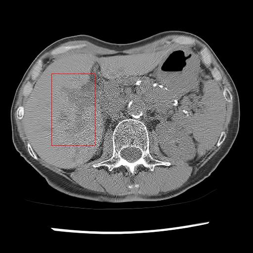
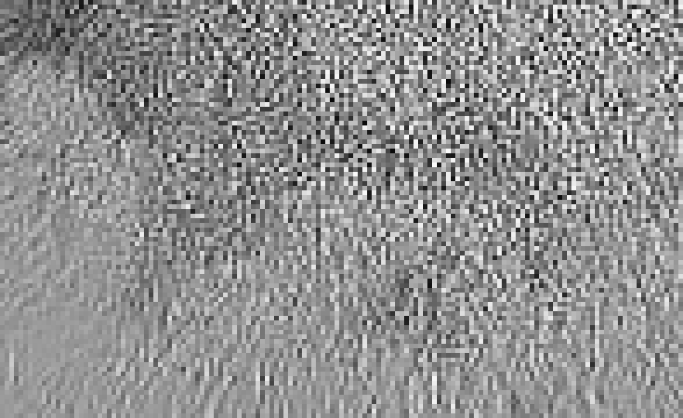
Here, we analyse the performance of the proposed method on clinical data. Since there are no ground truths available, only qualitative comparisons are performed. An example of the denoising performance of the proposed method is given in Figure 8. Here we can see denoising performance of BM3D is the worst compared to other methods. On the other hand, the output of the deep image prior is very blurry, different organ boundary is distorted, and some splotchy artifacts appear in the image. The performance of DIP depends mainly on the stopping iteration; with more iterations, it will again produce the original noisy image. The clean image produced by it is always blurry and without any texture. Consistent with our previous example, we can see CycleGAN has a lot of residual noise left in the example. Next, we identified one hypodense lesion in the image and marked the region with the red colour bounding box. The zoomed version of the region containing the lesion is shown in Figure 9. The effect of denoising is perceptible in this zoomed view. The visibility of the lesion is very inconspicuous in the original LDCT image. The noise variance is very high in this region; consequently, BM3D and CycleGAN failed to remove noise from this region. On the other hand, DIP has removed the noise but also destroyed the image by removing all the texture information. ConsensusNet also produced a blurry version of the lesion in the output. At the same time, our method produced a denoised image with the lowest granular pattern and improved the lesion’s visibility. The main objective of image denoising is to restore the visibility of these types of lesions and anomalies by concealing the noise. In this regard, our method has reached the goal as the perceptibility of different anomalies has been improved vastly without losing structural or textural information.

References

- [1] Joshua Batson and Loic Royer. Noise2self: Blind denoising by self-supervision. In International Conference on Machine Learning, pages 524–533. PMLR, 2019.
- [2] David J Brenner. Radiation risks potentially associated with low-dose ct screening of adult smokers for lung cancer. Radiology, 231(2):440–445, 2004.
- [3] Hu Chen, Yi Zhang, Mannudeep K Kalra, Feng Lin, Yang Chen, Peixi Liao, Jiliu Zhou, and Ge Wang. Low-dose ct with a residual encoder-decoder convolutional neural network. IEEE transactions on medical imaging, 36(12):2524–2535, 2017.
- [4] Kostadin Dabov, Alessandro Foi, Vladimir Katkovnik, and Karen Egiazarian. Image denoising with block-matching and 3d filtering. In Image Processing: Algorithms and Systems, Neural Networks, and Machine Learning, volume 6064, page 606414. International Society for Optics and Photonics, 2006.
- [5] Laurent Dinh, David Krueger, and Yoshua Bengio. Nice: Non-linear independent components estimation. arXiv preprint arXiv:1410.8516, 2014.
- [6] Laurent Dinh, Jascha Sohl-Dickstein, and Samy Bengio. Density estimation using real nvp. arXiv preprint arXiv:1605.08803, 2016.
- [7] Martin Heusel, Hubert Ramsauer, Thomas Unterthiner, Bernhard Nessler, and Sepp Hochreiter. Gans trained by a two time-scale update rule converge to a local nash equilibrium. Advances in neural information processing systems, 30, 2017.
- [8] Gao Huang, Zhuang Liu, Laurens Van Der Maaten, and Kilian Q Weinberger. Densely connected convolutional networks. In Proceedings of the IEEE conference on computer vision and pattern recognition, pages 4700–4708, 2017.
- [9] Zhiyuan Huang, Zixiang Chen, Qiyang Zhang, Guotao Quan, Min Ji, Chengjin Zhang, Yongfeng Yang, Xin Liu, Dong Liang, Hairong Zheng, et al. Cagan: A cycle-consistent generative adversarial network with attention for low-dose ct imaging. IEEE Transactions on Computational Imaging, 6:1203–1218, 2020.
- [10] Peter J Huber. Robust estimation of a location parameter. In Breakthroughs in statistics, pages 492–518. Springer, 1992.
- [11] Justin Johnson, Alexandre Alahi, and Li Fei-Fei. Perceptual losses for real-time style transfer and super-resolution. In European conference on computer vision, pages 694–711. Springer, 2016.
- [12] Diederik P Kingma and Prafulla Dhariwal. Glow: Generative flow with invertible 1x1 convolutions. arXiv preprint arXiv:1807.03039, 2018.
- [13] Alexander Krull, Tim-Oliver Buchholz, and Florian Jug. Noise2void-learning denoising from single noisy images. In Proceedings of the IEEE/CVF Conference on Computer Vision and Pattern Recognition, pages 2129–2137, 2019.
- [14] Taesung Kwon and Jong Chul Ye. Cycle-free cyclegan using invertible generator for unsupervised low-dose ct denoising. arXiv preprint arXiv:2104.08538, 2021.
- [15] Samuli Laine, Tero Karras, Jaakko Lehtinen, and Timo Aila. High-quality self-supervised deep image denoising. arXiv preprint arXiv:1901.10277, 2019.
- [16] Jaakko Lehtinen, Jacob Munkberg, Jon Hasselgren, Samuli Laine, Tero Karras, Miika Aittala, and Timo Aila. Noise2noise: Learning image restoration without clean data. arXiv preprint arXiv:1803.04189, 2018.
- [17] Zeheng Li, Junzhou Huang, Lifeng Yu, Yujie Chi, and Mingwu Jin. Low-dose ct image denoising using cycle-consistent adversarial networks. In 2019 IEEE Nuclear Science Symposium and Medical Imaging Conference (NSS/MIC), pages 1–3, 2019.
- [18] Zeheng Li, Shiwei Zhou, Junzhou Huang, Lifeng Yu, and Mingwu Jin. Investigation of low-dose ct image denoising using unpaired deep learning methods. IEEE Transactions on Radiation and Plasma Medical Sciences, 5(2):224–234, 2020.
- [19] Jingyun Liang, Andreas Lugmayr, Kai Zhang, Martin Danelljan, Luc Van Gool, and Radu Timofte. Hierarchical conditional flow: A unified framework for image super-resolution and image rescaling. In Proceedings of the IEEE/CVF International Conference on Computer Vision, pages 4076–4085, 2021.
- [20] Yang Liu, Zhenyue Qin, Saeed Anwar, Pan Ji, Dongwoo Kim, Sabrina Caldwell, and Tom Gedeon. Invertible denoising network: A light solution for real noise removal. In Proceedings of the IEEE/CVF Conference on Computer Vision and Pattern Recognition, pages 13365–13374, 2021.
- [21] Mehdi SM Sajjadi, Bernhard Scholkopf, and Michael Hirsch. Enhancenet: Single image super-resolution through automated texture synthesis. In Proceedings of the IEEE International Conference on Computer Vision, pages 4491–4500, 2017.
- [22] Alvin W Su, Travis J Hillen, Eric P Eutsler, Asheesh Bedi, James R Ross, Christopher M Larson, John C Clohisy, and Jeffrey J Nepple. Low-dose computed tomography reduces radiation exposure by 90% compared with traditional computed tomography among patients undergoing hip-preservation surgery. Arthroscopy: The Journal of Arthroscopic & Related Surgery, 35(5):1385–1392, 2019.
- [23] Dmitry Ulyanov, Andrea Vedaldi, and Victor Lempitsky. Deep image prior. In Proceedings of the IEEE conference on computer vision and pattern recognition, pages 9446–9454, 2018.
- [24] Tycho FA van der Ouderaa and Daniel E Worrall. Reversible gans for memory-efficient image-to-image translation. In Proceedings of the IEEE/CVF Conference on Computer Vision and Pattern Recognition, pages 4720–4728, 2019.
- [25] Dufan Wu, Kuang Gong, Kyungsang Kim, Xiang Li, and Quanzheng Li. Consensus neural network for medical imaging denoising with only noisy training samples. In International Conference on Medical Image Computing and Computer-Assisted Intervention, pages 741–749. Springer, 2019.
- [26] Mingqing Xiao, Shuxin Zheng, Chang Liu, Yaolong Wang, Di He, Guolin Ke, Jiang Bian, Zhouchen Lin, and Tie-Yan Liu. Invertible image rescaling. In European Conference on Computer Vision, pages 126–144. Springer, 2020.
- [27] Guorong Xuan, Chengyun Yang, Yizhan Zhen, Yun Q Shi, and Zhicheng Ni. Reversible data hiding based on wavelet spread spectrum. In IEEE 6th Workshop on Multimedia Signal Processing, 2004., pages 211–214. IEEE, 2004.
- [28] Rui Zhao, Tianshan Liu, Jun Xiao, Daniel PK Lun, and Kin-Man Lam. Invertible image decolorization. IEEE Transactions on Image Processing, 30:6081–6095, 2021.
- [29] Jun-Yan Zhu, Taesung Park, Phillip Isola, and Alexei A Efros. Unpaired image-to-image translation using cycle-consistent adversarial networks. In Proceedings of the IEEE international conference on computer vision, pages 2223–2232, 2017.