Self-Supervised Aggregation of Diverse Experts for Test-Agnostic Long-Tailed Recognition
Abstract
Existing long-tailed recognition methods, aiming to train class-balanced models from long-tailed data, generally assume the models would be evaluated on the uniform test class distribution. However, practical test class distributions often violate this assumption (e.g., being either long-tailed or even inversely long-tailed), which may lead existing methods to fail in real applications. In this paper, we study a more practical yet challenging task, called test-agnostic long-tailed recognition, where the training class distribution is long-tailed while the test class distribution is agnostic and not necessarily uniform. In addition to the issue of class imbalance, this task poses another challenge: the class distribution shift between the training and test data is unknown. To tackle this task, we propose a novel approach, called Self-supervised Aggregation of Diverse Experts, which consists of two strategies: (i) a new skill-diverse expert learning strategy that trains multiple experts from a single and stationary long-tailed dataset to separately handle different class distributions; (ii) a novel test-time expert aggregation strategy that leverages self-supervision to aggregate the learned multiple experts for handling unknown test class distributions. We theoretically show that our self-supervised strategy has a provable ability to simulate test-agnostic class distributions. Promising empirical results demonstrate the effectiveness of our method on both vanilla and test-agnostic long-tailed recognition. Code is available at https://github.com/Vanint/SADE-AgnosticLT.
1 Introduction
Real-world visual recognition datasets typically exhibit a long-tailed distribution, where a few classes contain numerous samples (called head classes), but the others are associated with only a few instances (called tail classes) kang2021exploring ; menon2020long . Due to the class imbalance, the trained model is easily biased towards head classes and perform poorly on tail classes cai2021ace ; zhang2021deep . To tackle this issue, numerous studies have explored long-tailed recognition for learning well-performing models from imbalanced data jamal2020rethinking ; zhang2021distribution .
Most existing long-tailed studies cao2019learning ; cui2019class ; deng2021pml ; wang2021contrastive ; weng2021unsupervised assume the test class distribution is uniform, i.e., each class has an equal amount of test data. Therefore, they develop various techniques, e.g., class re-sampling guo2021long ; huang2016learning ; kang2019decoupling ; zang2021fasa , cost-sensitive learning feng2021exploring ; Influence2021Park ; tan2020equalization ; wang2021seesaw or ensemble learning cai2021ace ; guo2021long ; li2020overcoming ; xiang2020learning , to re-balance the model performance on different classes for fitting the uniform class distribution. However, this assumption does not always hold in real applications, where actual test data may follow any kind of class distribution, being either uniform, long-tailed, or even inversely long-tailed to the training data (cf. Figure 1(a)). For example, one may train a recognition model for autonomous cars based on the training data collected from city areas, where pedestrians are majority classes and stone obstacles are minority classes. However, when the model is deployed to mountain areas, the pedestrians become the minority while the stones become the majority. In this case, the test class distribution is inverse to the training one, and existing methods may perform poorly.

(a) Existing long-tailed recognition methods
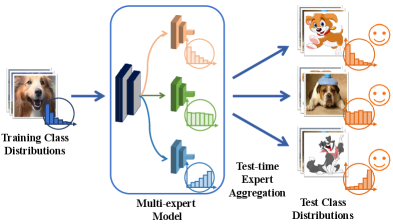
(b) The idea of our proposed method
To address the issue of varying class distributions, as the first research attempt, LADE hong2020disentangling assumes the test class distribution to be known and uses the knowledge to post-adjust model predictions. However, the actual test class distribution is usually unknown a priori, making LADE not applicable in practice. Therefore, we study a more realistic yet challenging problem, namely test-agnostic long-tailed recognition, where the training class distribution is long-tailed while the test distribution is agnostic. To tackle this problem, motivated by the idea of "divide and conquer", we propose to learn multiple experts with diverse skills that excel at handling different class distributions (cf. Figure 1(b)). As long as these skill-diverse experts can be aggregated suitably at test time, the multi-expert model would manage to handle the unknown test class distribution. Following this idea, we develop a novel approach, namely Self-supervised Aggregation of Diverse Experts (SADE).
The first challenge for SADE is how to learn multiple diverse experts from a single and stationary long-tailed training dataset. To handle this challenge, we empirically evaluate existing long-tailed methods in this task, and find that the models trained by existing methods have a simulation correlation between the learned class distribution and the training loss function. That is, the models learned by various losses are skilled in handling class distributions with different skewness. For example, the model trained with the conventional softmax loss simulates the long-tailed training class distribution, while the models obtained from existing long-tailed methods are good at the uniform class distribution. Inspired by this finding, SADE presents a simple but effective skill-diverse expert learning strategy to generate experts with different distribution preferences from a single long-tailed training distribution. Here, various experts are trained with different expertise-guided objective functions to deal with different class distributions, respectively. As a result, the learned experts are more diverse than previous multi-expert long-tailed methods wang2020long ; zhou2020bbn , leading to better ensemble performance, and in aggregate simulate a wide spectrum of possible class distributions.
The other challenge is how to aggregate these skill-diverse experts for handling test-agnostic class distributions based on only unlabeled test data. To tackle this challenge, we empirically investigate the property of different experts, and observe that there is a positive correlation between expertise and prediction stability, i.e., stronger experts have higher prediction consistency between different perturbed views of samples from their favorable classes. Motivated by this finding, we develop a novel self-supervised strategy, namely prediction stability maximization, to adaptively aggregate experts based on only unlabeled test data. We theoretically show that maximizing the prediction stability enables SADE to learn an aggregation weight that maximizes the mutual information between the predicted label distribution and the true class distribution. In this way, the resulting model is able to simulate unknown test class distributions.
We empirically verify the superiority of SADE on both vanilla and test-agnostic long-tailed recognition. Specifically, SADE achieves promising performance on vanilla long-tailed recognition under all benchmark datasets. For instance, SADE achieves 58.8 accuracy on ImageNet-LT with more than 2 accuracy gain over previous state-of-the-art ensemble long-tailed methods, i.e., RIDE wang2020long and ACE cai2021ace . More importantly, SADE is the first long-tailed approach that is able to handle various test-agnostic class distributions without knowing the true class distribution of test data in advance. Note that SADE even outperforms LADE hong2020disentangling that uses knowledge of the test class distribution.
Compared to previous long-tailed methods (e.g., LADE hong2020disentangling and RIDE wang2020long ), our method offers the following advantages: (i) SADE does not assume the test class distribution to be known, and provides the first practical approach to handling test-agnostic long-tailed recognition; (ii) SADE develops a simple diversity-promoting strategy to learn skill-diverse experts from a single and stationary long-tailed dataset; (iii) SADE presents a novel self-supervised strategy to aggregate skill-diverse experts at test time, by maximizing prediction consistency between unlabeled test samples’ perturbed views; (iv) the presented self-supervised strategy has a provable ability to simulate test-agnostic class distributions, which opens the opportunity for tackling unknown class distribution shifts at test time.
2 Related Work
Long-tailed recognition Existing long-tailed recognition methods, related to our study, can be categorized into three types: class re-balancing, logit adjustment and ensemble learning. Specifically, class re-balancing resorts to re-sampling chawla2002smote ; guo2021long ; huang2016learning ; kang2019decoupling or cost-sensitive learning cao2019learning ; deng2021pml ; he2022relieving ; zhao2018adaptive to balance different classes during model training. Logit adjustment hong2020disentangling ; menon2020long ; peng2021optimal ; tian2020posterior adjusts models’ output logits via the label frequencies of training data at inference time, for obtaining a large relative margin between head and tail classes. Ensemble-based methods cai2021ace ; guo2021long ; xiang2020learning ; zhou2020bbn , e.g., RIDE wang2020long , are based on multiple experts, which seek to capture heterogeneous knowledge, followed by ensemble aggregation. More discussions on the difference between our method and RIDE wang2020long are provided in Appendix D.3. Regarding test-agnostic long-tailed recognition, LADE hong2020disentangling assumes the test class distribution is available and uses it to post-adjust model predictions. However, the true test class distribution is usually unknown a priori, making LADE inapplicable. In contrast, our method does not rely on the true test distribution for handling this problem, but presents a novel self-supervised strategy to aggregate skill-diverse experts at test time for test-agnostic class distributions. Moreover, some ensemble-based long-tailed methods sharma2020long aggregate experts based on a labeled uniform validation set. However, as the test class distribution could be different from the validation one, simply aggregating experts on the validation set is unable to handle test-agnostic long-tailed recognition.
Test-time training Test-time training kamani2020targeted ; kim2020learning ; liu2021ttt++ ; sun2020test ; wang2021tent is a transductive learning paradigm for handling distribution shifts lin2022prototype ; long2014transfer ; niu2022efficient ; qiu2021source ; varsavsky2020test ; zhang2020collaborative between training and test data, and has been applied with success to out-of-domain generalization iwasawa2021test ; pandey2021generalization and dynamic scene deblurring chi2021test . In this study, we explore this paradigm to handle test-agnostic long-tailed recognition, where the issue of class distribution shifts is the main challenge. However, most existing test-time training methods seek to handle covariate distribution shifts instead of class distribution shifts, so simply leveraging them cannot resolve test-agnostic long-tailed recognition, as shown in our experiment (cf. Table 9).
3 Problem Formulation
Long-tailed recognition aims to learn a well-performing classification model from a training dataset with long-tailed class distribution. Let denote the long-tailed training set, where is the class label of the sample . The total number of training data over classes is , where denotes the number of samples in class . Without loss of generality, we follow a common assumption hong2020disentangling ; kang2019decoupling that the classes are sorted by cardinality in decreasing order (i.e., if , then ), and . The imbalance ratio is defined as //. The test data is defined in a similar way.
Most existing long-tailed recognition methods assume the test class distribution is uniform (i.e., ), and seek to train models from the long-tailed training distribution to perform well on the uniform test distribution. However, such an assumption does not always hold in practice. The actual test class distribution in real-world applications may also be long-tailed (i.e., ), or even inversely long-tailed to the training data (i.e., ). Here, indicates that the order of the long tail on classes is flipped. As a result, the models learned by existing methods may fail when the actual test class distribution is different from the assumed one. To address this, we propose to study a more practical yet challenging long-tailed problem, i.e., Test-agnostic Long-tailed Recognition. This task aims to learn a recognition model from long-tailed training data, where the resulting model would be evaluated on multiple test sets that follow different class distributions. This task is challenging due to the integration of two challenges: (1) the severe class imbalance in the training data makes it difficult to train models; (2) unknown class distribution shifts between training and test data (i.e., ) makes models hard to generalize.
| Test class distribution | Softmax | Balanced Softmax jiawei2020balanced | LADE w/o prior hong2020disentangling | ||||||||
|---|---|---|---|---|---|---|---|---|---|---|---|
| Many | Medium | Few | Many | Medium | Few | Many | Medium | Few | |||
| Forward-LT-50 | 67.5 | 41.7 | 14.0 | 63.5 | 47.8 | 37.5 | 63.5 | 46.4 | 33.1 | ||
| Forward-LT-10 | 68.2 | 40.9 | 14.0 | 64.1 | 48.2 | 31.2 | 64.7 | 47.1 | 32.2 | ||
| Uniform | 68.1 | 41.5 | 14.0 | 64.1 | 48.2 | 33.4 | 64.4 | 47.7 | 34.3 | ||
| Backward-LT-10 | 67.4 | 41.9 | 13.9 | 63.4 | 49.1 | 33.6 | 64.4 | 48.2 | 34.2 | ||
| Backward-LT-50 | 70.9 | 41.1 | 13.8 | 66.5 | 48.4 | 33.2 | 66.3 | 47.8 | 34.0 | ||
4 Method
To tackle the above problem, inspired by the idea of "divide and conquer", we propose to learn multiple skill-diverse experts that excel at handling different class distributions. By reasonably fusing these experts at test time, the multi-expert model would manage to handle unknown class distribution shifts and resolve test-agnostic long-tailed recognition. Following this idea, we develop a novel Self-supervised Aggregation of Diverse Experts (SADE) approach. Specifically, SADE consists of two innovative strategies: (1) learning skill-diverse experts from a single long-tailed training dataset; (2) test-time aggregating experts with self-supervision to handle test-agnostic class distributions.
4.1 Skill-diverse Expert Learning
As shown in Figure 2, SADE builds a three-expert model that comprises two components: (1) an expert-shared backbone ; (2) independent expert networks , and . When training the model, the key challenge is how to learn skill-diverse experts from a single and stationary long-tailed training dataset. Existing ensemble-based long-tailed methods guo2021long ; wang2020long seek to train experts for the uniform test class distribution, and hence the trained experts are not differentiated sufficiently for handling various class distributions (refer to Table 6 for an example). To tackle this challenge, we first empirically investigate existing long-tailed methods in this task. From Table 1, we find that there is a simulation correlation between the learned class distribution and the training loss function. That is, the models learned by different losses are good at dealing with class distributions with different skewness. For instance, the model trained with the softmax loss is good at the long-tailed distribution, while the models obtained from long-tailed methods are skilled in the uniform distribution.
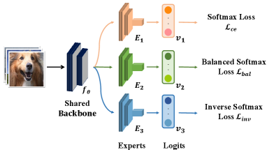
Motivated by this finding, we develop a simple skill-diverse expert learning strategy to generate experts with different distribution preferences. To be specific, the forward expert seeks to be good at the long-tailed class distribution and performs well on many-shot classes. The uniform expert strives to be skilled in the uniform distribution. The backward expert aims at the inversely long-tailed distribution and performs well on few-shot classes. Here, the forward and backward experts are necessary since they span a wide spectrum of possible class distributions, while the uniform expert ensures retaining high accuracy on the uniform distribution. To this end, we use three different expertise-guided losses to train the three experts, respectively.
The forward expert We use the softmax cross-entropy loss to train this expert, so that it directly simulates the original long-tailed training class distribution:
| (1) |
where is the output logits of the forward expert , and is the softmax function.
The uniform expert We aim to train this expert to simulate the uniform class distribution. Inspired by the effectiveness of logit adjusted losses for long-tailed recognition menon2020long , we resort to the balanced softmax loss jiawei2020balanced . Specifically, let be the prediction probability. The balanced softmax adjusts the prediction probability by compensating for the long-tailed class distribution with the prior of training label frequencies: , where denotes the training label frequency of class . Then, given as the output logits of the expert , the balanced softmax loss for the expert is defined as:
| (2) |
Intuitively, by adjusting logits to compensate for the long-tailed distribution with the prior , this loss enables to output class-balanced predictions that simulate the uniform distribution.
The backward expert We seek to train this expert to simulate the inversely long-tailed class distribution. To this end, we propose a new inverse softmax loss, based on the same rationale of logit adjusted losses jiawei2020balanced ; menon2020long . Specifically, we adjust the prediction probability by: , where the inverse training prior is obtained by inverting the order of training label frequencies . Then, the new inverse softmax loss for the expert is defined as:
| (3) |
where denotes the output logits of and is a hyper-parameter. Intuitively, this loss adjusts logits to compensate for the long-tailed distribution with , and further applies reverse adjustment with . This enables to simulate the inversely long-tailed distribution (cf. Table 6 for verification).
4.2 Test-time Self-supervised Aggregation
Based on the skill-diverse learning strategy, the three experts in SADE are skilled in different class distributions. The remaining challenge is how to fuse them to deal with unknown test class distributions. A basic principle for expert aggregation is that the experts should play a bigger role in situations where they have expertise. Nevertheless, how to detect strong experts for unknown test class distribution remains unknown. Our key insight is that strong experts should be more stable in predicting the samples from their skilled classes, even though these samples are perturbed.
Empirical observation To verify this hypothesis, we estimate the prediction stability of experts by comparing the cosine similarity between their predictions for a sample’s two augmented views. Here, the data views are generated by the data augmentation techniques in MoCo v2 chen2020improved . From Table 2, we find that there is a positive correlation between expertise and prediction stability, i.e., stronger experts have higher prediction similarity between different views of samples from their favorable classes. Following this finding, we propose to explore the relative prediction stability to detect strong experts and weight experts for the unknown test class distribution. Consequently, we develop a novel self-supervised strategy, namely prediction stability maximization.
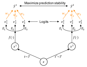
Prediction stability maximization This strategy learns aggregation weights for experts (with frozen parameters) by maximizing model prediction stability for unlabeled test samples. As shown in Figure 2, the method comprises three major components as follows.
Data view generation For a given sample , we conduct two stochastic data augmentations to generate the sample’s two views, i.e., and . Here, we use the same augmentation techniques as the advanced contrastive learning method, i.e., MoCo v2 chen2020improved , which has been shown effective in self-supervised learning.
Learnable aggregation weight Given the output logits of three experts , we aggregate experts with a learnable aggregation weight and obtain the final softmax prediction by , where is normalized before aggregation, i.e., .
Objective function Given the view predictions of unlabeled test data, we maximize the prediction stability based on the cosine similarity between the view predictions:
| (4) |
Here, and are normalized by the softmax function. In test-time training, only the aggregation weight is updated. Since stronger experts have higher prediction similarity for their skilled classes, maximizing the prediction stability would learn higher weights for stronger experts regarding the unknown test class distribution. Moreover, the self-supervised aggregation strategy can be conducted in an online manner for streaming test data. The pseudo-code of SADE is provided in Appendix B.
| Model | Cosine similarity between view predictions | ||||||
|---|---|---|---|---|---|---|---|
| ImageNet-LT | CIFAR100-LT | ||||||
| Many | Med. | Few | Many | Med. | Few | ||
| Expert | 0.60 | 0.48 | 0.43 | 0.28 | 0.22 | 0.20 | |
| Expert | 0.56 | 0.50 | 0.45 | 0.25 | 0.21 | 0.19 | |
| Expert | 0.52 | 0.53 | 0.58 | 0.22 | 0.23 | 0.25 | |
Theoretical Analysis We then theoretically analyze the prediction stability maximization strategy to conceptually understand why it works. To this end, we first define the random variables of predictions and labels as and . We have the following result:
Theorem 1.
The prediction stability is positive proportional to the mutual information between the predicted label distribution and the test class distribution , and negative proportional to the prediction entropy :
Please refer to Appendix A for proofs. According to Theorem 1, maximizing the prediction stability enables SADE to learn an aggregation weight that maximizes the mutual information between the predicted label distribution and the test class distribution , as well as minimizing the prediction entropy. Since minimizing entropy helps to improve the confidence of the classifier output grandvalet2005semi , the aggregation weight is learned to simulate the test class distribution and increase the prediction confidence. This property intuitively explains why our method has the potential to tackle the challenging task of test-agnostic long-tailed recognition at test time.
5 Experiments
In this section, we first evaluate the superiority of SADE on both vanilla and test-agnostic long-tailed recognition. We then verify the effectiveness of SADE in terms of its two strategies, i.e., skill-diverse expert learning and test-time self-supervised aggregation. More ablation studies are reported in appendices. Here, we begin with the experimental settings.
5.1 Experimental Setups
Datasets We use four benchmark datasets (i.e., ImageNet-LT liu2019large , CIFAR100-LT cao2019learning , Places-LT liu2019large , and iNaturalist 2018 van2018inaturalist ) to simulate real-world long-tailed class distributions. Their data statistics and imbalance ratios are summarized in Appendix C.1. The imbalance ratio is defined as /, where denotes the data number of class . Note that CIFAR100-LT has three variants with different imbalance ratios.
Baselines We compare SADE with state-of-the-art long-tailed methods, including two-stage methods (Decouple kang2019decoupling , MiSLAS zhong2021improving ), logit-adjusted training (Balanced Softmax jiawei2020balanced , LADE hong2020disentangling ), ensemble learning (BBN zhou2020bbn , ACE cai2021ace , RIDE wang2020long ), classifier design (Causal tang2020long ), and representation learning (PaCo cui2021parametric ). Note that LADE uses the prior of test class distribution for post-adjustment (although it is unavailable in practice), while all other methods do not use this prior.
Evaluation protocols In test-agnostic long-tailed recognition, following LADE hong2020disentangling , the models are evaluated on multiple sets of test data that follow different class distributions, in terms of micro accuracy. Same as LADE hong2020disentangling , we construct three kinds of test class distributions, i.e., the uniform distribution, forward long-tailed distributions as training data, and backward long-tailed distributions. In the backward ones, the order of the long tail on classes is flipped. More details of test data construction are provided in Appendix C.2. Besides, we also evaluate methods on vanilla long-tailed recognition kang2019decoupling ; liu2019large , where the models are evaluated on the uniform test class distribution. Here, the accuracy on three class sub-groups is also reported, i.e., many-shot classes (more than 100 training images), medium-shot classes (20100 images) and few-shot classes (less than 20 images).
Implementation details We use the same setup for all the baselines and our method. Specifically, following hong2020disentangling ; wang2020long , we use ResNeXt-50 for ImageNet-LT, ResNet-32 for CIFAR100-LT, ResNet-152 for Places-LT and ResNet-50 for iNaturalist 2018 as backbones, respectively. Moreover, we adopt the cosine classifier for prediction on all datasets. If not specified, we use the SGD optimizer with the momentum of 0.9 for training 200 epochs and set the initial learning rate as 0.1 with linear decay. We set for ImageNet-LT and CIFAR100-LT, and for the remaining datasets. During test-time training, we train the aggregation weights for 5 epochs with the batch size 128, where we use the same optimizer and learning rate as the training phase. More implementation details and the hyper-parameter statistics are reported in Appendix C.3.
(a) CIFAR100-LT
| Imbalance Ratio | 10 | 50 | 100 |
|---|---|---|---|
| Softmax | 59.1 | 45.6 | 41.4 |
| BBN zhou2020bbn | 59.8 | 49.3 | 44.7 |
| Causal tang2020long | 59.4 | 48.8 | 45.0 |
| Balanced Softmax jiawei2020balanced | 61.0 | 50.9 | 46.1 |
| MiSLAS zhong2021improving | 62.5 | 51.5 | 46.8 |
| LADE hong2020disentangling | 61.6 | 50.1 | 45.6 |
| RIDE wang2020long | 61.8 | 51.7 | 48.0 |
| SADE (ours) | 63.6 | 53.9 | 49.8 |
(b) Places-LT
| Method | Top-1 accuracy |
|---|---|
| Softmax | 31.4 |
| Causal tang2020long | 32.2 |
| Balanced Softmax jiawei2020balanced | 39.4 |
| MiSLAS zhong2021improving | 38.3 |
| LADE hong2020disentangling | 39.2 |
| RIDE wang2020long | 40.3 |
| SADE (ours) | 40.9 |
(c) iNaturalist 2018
| Method | Top-1 accuracy |
|---|---|
| Softmax | 64.7 |
| Causal tang2020long | 64.4 |
| Balanced Softmax jiawei2020balanced | 70.6 |
| MiSLAS zhong2021improving | 70.7 |
| LADE hong2020disentangling | 69.3 |
| RIDE wang2020long | 71.8 |
| SADE (ours) | 72.9 |
| Method | Many | Med. | Few | All |
|---|---|---|---|---|
| Softmax | 68.1 | 41.5 | 14.0 | 48.0 |
| Decouple-LWS kang2019decoupling | 61.8 | 47.6 | 30.9 | 50.8 |
| Causal tang2020long | 64.1 | 45.8 | 27.2 | 50.3 |
| Balanced Softmax jiawei2020balanced | 64.1 | 48.2 | 33.4 | 52.3 |
| MiSLAS zhong2021improving | 62.0 | 49.1 | 32.8 | 51.4 |
| LADE hong2020disentangling | 64.4 | 47.7 | 34.3 | 52.3 |
| PaCo cui2021parametric | 63.2 | 51.6 | 39.2 | 54.4 |
| ACE cai2021ace | 71.7 | 54.6 | 23.5 | 56.6 |
| RIDE wang2020long | 68.0 | 52.9 | 35.1 | 56.3 |
| SADE (ours) | 66.5 | 57.0 | 43.5 | 58.8 |
5.2 Superiority on Vanilla Long-tailed Recognition
This subsection compares SADE with state-of-the-art long-tailed methods on vanilla long-tailed recognition. Specifically, as shown in Tables 3-4, Softmax trains the model with only cross-entropy, so it simulates the long-tailed training distribution and performs well on many-shot classes. However, it performs poorly on medium-shot and few-shot classes, leading to worse overall performance. In contrast, existing long-tailed methods (e.g., Decouple, Causal) seek to simulate the uniform class distribution, so their performance is more class-balanced, leading to better overall performance. However, as these methods mainly seek balanced performance, they inevitably sacrifice the performance on many-shot classes. To address this, RIDE and ACE explore ensemble learning for long-tailed recognition and achieve better performance on tail classes without sacrificing the head-class performance. In comparison, based on the increasing expert diversity derived from skill-diverse expert learning, our method performs the best on all datasets, e.g., with more than 2 accuracy gain on ImageNet-LT compared to RIDE and ACE. These results demonstrate the superiority of SADE over the compared methods that are particularly designed for the uniform test class distribution. Note that SADE also outperforms baselines in experiments with stronger data augmentation (i.e., RandAugment cubuk2020randaugment ) and other architectures, as reported in Appendix D.1.
5.3 Superiority on Test-agnostic Long-tailed Recognition
In this subsection, we evaluate SADE on test-agnostic long-tailed recognition. The results on various test class distributions are reported in Table 5. Specifically, since Softmax seeks to simulate the long-tailed training distribution, it performs well on forward long-tailed test distributions. However, its performance on the uniform and backward long-tailed distributions is poor. In contrast, existing long-tailed methods show more balanced performance among classes, leading to better overall accuracy. However, the resulting models by these methods suffer from a simulation bias, i.e., performing similarly among classes on various class distributions (c.f. Table 1). As a result, they cannot adapt to diverse test class distributions well. To handle this task, LADE assumes the test class distribution to be known and uses this information to adjust its predictions, leading to better performance on various test class distributions. However, since obtaining the actual test class distribution is difficult in real applications, the methods requiring such knowledge may be not applicable in practice. Moreover, in some specific cases like Forward-LT-3 and Backward-LT-3 distributions of iNaturalist 2018, the number of test samples on some classes becomes zero. In such cases, the test prior cannot be used in LADE, since adjusting logits with results in biased predictions. In contrast, without relying on the knowledge of test class distributions, our SADE presents an innovative self-supervised strategy to deal with unknown class distributions, and obtains even better performance than LADE that uses the test class prior (c.f. Table 5). The promising results demonstrate the effectiveness and practicality of our method on test-agnostic long-tailed recognition. Note that the performance advantages of SADE become larger as the test data get more imbalanced. Due to the page limitation, the results on more datasets are reported in Appendix D.2.
| Method | Prior | (a) ImageNet-LT | (b) CIFAR100-LT (IR100) | |||||||||||||||||||||||||
|---|---|---|---|---|---|---|---|---|---|---|---|---|---|---|---|---|---|---|---|---|---|---|---|---|---|---|---|---|
| Forward-LT | Uni. | Backward-LT | Forward-LT | Uni. | Backward-LT | |||||||||||||||||||||||
| 50 | 25 | 10 | 5 | 2 | 1 | 2 | 5 | 10 | 25 | 50 | 50 | 25 | 10 | 5 | 2 | 1 | 2 | 5 | 10 | 25 | 50 | |||||||
| Softmax | ✗ | 66.1 | 63.8 | 60.3 | 56.6 | 52.0 | 48.0 | 43.9 | 38.6 | 34.9 | 30.9 | 27.6 | 63.3 | 62.0 | 56.2 | 52.5 | 46.4 | 41.4 | 36.5 | 30.5 | 25.8 | 21.7 | 17.5 | |||||
| BS | ✗ | 63.2 | 61.9 | 59.5 | 57.2 | 54.4 | 52.3 | 50.0 | 47.0 | 45.0 | 42.3 | 40.8 | 57.8 | 55.5 | 54.2 | 52.0 | 48.7 | 46.1 | 43.6 | 40.8 | 38.4 | 36.3 | 33.7 | |||||
| MiSLAS | ✗ | 61.6 | 60.4 | 58.0 | 56.3 | 53.7 | 51.4 | 49.2 | 46.1 | 44.0 | 41.5 | 39.5 | 58.8 | 57.2 | 55.2 | 53.0 | 49.6 | 46.8 | 43.6 | 40.1 | 37.7 | 33.9 | 32.1 | |||||
| LADE | ✗ | 63.4 | 62.1 | 59.9 | 57.4 | 54.6 | 52.3 | 49.9 | 46.8 | 44.9 | 42.7 | 40.7 | 56.0 | 55.5 | 52.8 | 51.0 | 48.0 | 45.6 | 43.2 | 40.0 | 38.3 | 35.5 | 34.0 | |||||
| LADE | ✓ | 65.8 | 63.8 | 60.6 | 57.5 | 54.5 | 52.3 | 50.4 | 48.8 | 48.6 | 49.0 | 49.2 | 62.6 | 60.2 | 55.6 | 52.7 | 48.2 | 45.6 | 43.8 | 41.1 | 41.5 | 40.7 | 41.6 | |||||
| RIDE | ✗ | 67.6 | 66.3 | 64.0 | 61.7 | 58.9 | 56.3 | 54.0 | 51.0 | 48.7 | 46.2 | 44.0 | 63.0 | 59.9 | 57.0 | 53.6 | 49.4 | 48.0 | 42.5 | 38.1 | 35.4 | 31.6 | 29.2 | |||||
| SADE | ✗ | 69.4 | 67.4 | 65.4 | 63.0 | 60.6 | 58.8 | 57.1 | 55.5 | 54.5 | 53.7 | 53.1 | 65.9 | 62.5 | 58.3 | 54.8 | 51.1 | 49.8 | 46.2 | 44.7 | 43.9 | 42.5 | 42.4 | |||||
| Method | Prior | (c) Places-LT | (d) iNaturalist 2018 | |||||||||||||||||||||||||
| Forward-LT | Uni. | Backward-LT | Forward-LT | Uni. | Backward-LT | |||||||||||||||||||||||
| 50 | 25 | 10 | 5 | 2 | 1 | 2 | 5 | 10 | 25 | 50 | 3 | 2 | 1 | 2 | 3 | |||||||||||||
| Softmax | ✗ | 45.6 | 42.7 | 40.2 | 38.0 | 34.1 | 31.4 | 28.4 | 25.4 | 23.4 | 20.8 | 19.4 | 65.4 | 65.5 | 64.7 | 64.0 | 63.4 | |||||||||||
| BS | ✗ | 42.7 | 41.7 | 41.3 | 41.0 | 40.0 | 39.4 | 38.5 | 37.8 | 37.1 | 36.2 | 35.6 | 70.3 | 70.5 | 70.6 | 70.6 | 70.8 | |||||||||||
| MiSLAS | ✗ | 40.9 | 39.7 | 39.5 | 39.6 | 38.8 | 38.3 | 37.3 | 36.7 | 35.8 | 34.7 | 34.4 | 70.8 | 70.8 | 70.7 | 70.7 | 70.2 | |||||||||||
| LADE | ✗ | 42.8 | 41.5 | 41.2 | 40.8 | 39.8 | 39.2 | 38.1 | 37.6 | 36.9 | 36.0 | 35.7 | 68.4 | 69.0 | 69.3 | 69.6 | 69.5 | |||||||||||
| LADE | ✓ | 46.3 | 44.2 | 42.2 | 41.2 | 39.7 | 39.4 | 39.2 | 39.9 | 40.9 | 42.4 | 43.0 | ✗ | 69.1 | 69.3 | 70.2 | ✗ | |||||||||||
| RIDE | ✗ | 43.1 | 41.8 | 41.6 | 42.0 | 41.0 | 40.3 | 39.6 | 38.7 | 38.2 | 37.0 | 36.9 | 71.5 | 71.9 | 71.8 | 71.9 | 71.8 | |||||||||||
| SADE | ✗ | 46.4 | 44.9 | 43.3 | 42.6 | 41.3 | 40.9 | 40.6 | 41.1 | 41.4 | 42.0 | 41.6 | 72.3 | 72.5 | 72.9 | 73.5 | 73.3 | |||||||||||
| Model | RIDE wang2020long | SADE (ours) | |||||||||||||||||
|---|---|---|---|---|---|---|---|---|---|---|---|---|---|---|---|---|---|---|---|
| ImageNet-LT | CIFAR100-LT | ImageNet-LT | CIFAR100-LT | ||||||||||||||||
| Many | Med. | Few | All | Many | Med. | Few | All | Many | Med. | Few | All | Many | Med. | Few | All | ||||
| Expert | 64.3 | 49.0 | 31.9 | 52.6 | 63.5 | 44.8 | 20.3 | 44.0 | 68.8 | 43.7 | 17.2 | 49.8 | 67.6 | 36.3 | 6.8 | 38.4 | |||
| Expert | 64.7 | 49.4 | 31.2 | 52.8 | 63.1 | 44.7 | 20.2 | 43.8 | 65.5 | 50.5 | 33.3 | 53.9 | 61.2 | 44.7 | 23.5 | 44.2 | |||
| Expert | 64.3 | 48.9 | 31.8 | 52.5 | 63.9 | 45.1 | 20.5 | 44.3 | 43.4 | 48.6 | 53.9 | 47.3 | 14.0 | 27.6 | 41.2 | 25.8 | |||
| Ensemble | 68.0 | 52.9 | 35.1 | 56.3 | 67.4 | 49.5 | 23.7 | 48.0 | 67.0 | 56.7 | 42.6 | 58.8 | 61.6 | 50.5 | 33.9 | 49.4 | |||
5.4 Effectiveness of Skill-diverse Expert Learning
We next examine our skill-diverse expert learning strategy. The results are reported in Table 6, where RIDE wang2020long is a state-of-the-art ensemble-based method. RIDE trains each expert with cross-entropy independently and uses KL-Divergence to improve expert diversity. However, simply maximizing the divergence of expert predictions cannot learn visibly diverse experts (cf. Table 6). In contrast, the three experts learned by our strategy have significantly diverse expertise, excelling at many-shot classes, the uniform distribution (with higher overall performance), and few-shot classes, respectively. As a result, the increasing expert diversity leads to a non-trivial gain for the ensemble performance of SADE compared to RIDE. Moreover, consistent results on more datasets are reported in Appendix D.3, while the ablation studies of the expert learning strategy are provided in Appendix E.
| Test Dist. | Expert () | Expert () | Expert () |
|---|---|---|---|
| Forward-LT-50 | 0.52 | 0.35 | 0.13 |
| Forward-LT-10 | 0.46 | 0.36 | 0.18 |
| Uniform | 0.33 | 0.33 | 0.34 |
| Backward-LT-10 | 0.21 | 0.29 | 0.50 |
| Backward-LT-50 | 0.17 | 0.27 | 0.56 |
| Test Dist. | ImageNet-LT | ||||||||
| Ours w/o test-time strategy | Ours w/ test-time strategy | ||||||||
| Many | Med. | Few | All | Many | Med. | Few | All | ||
| Forward-LT-50 | 65.6 | 55.7 | 44.1 | 65.5 | 70.0 | 53.2 | 33.1 | 69.4 (+3.9) | |
| Forward-LT-10 | 66.5 | 56.8 | 44.2 | 63.6 | 69.9 | 54.3 | 34.7 | 65.4 (+1.8) | |
| Uniform | 67.0 | 56.7 | 42.6 | 58.8 | 66.5 | 57.0 | 43.5 | 58.8 (+0.0) | |
| Backward-LT-10 | 65.0 | 57.6 | 43.1 | 53.1 | 60.9 | 57.5 | 50.1 | 54.5 (+1.4) | |
| Backward-LT-50 | 69.1 | 57.0 | 42.9 | 49.8 | 60.7 | 56.2 | 50.7 | 53.1 (+3.3) | |
| Backbone | Test-time strategy | Forward | Uniform | Backward | ||||||||||
|---|---|---|---|---|---|---|---|---|---|---|---|---|---|---|
| 50 | 25 | 10 | 5 | 2 | 1 | 2 | 5 | 10 | 25 | 50 | ||||
| SADE | No test-time adaptation | 65.5 | 64.4 | 63.6 | 62.0 | 60.0 | 58.8 | 56.8 | 54.7 | 53.1 | 51.5 | 49.8 | ||
| Test-time pseudo-labeling | 67.1 | 66.1 | 64.7 | 63.0 | 60.1 | 57.7 | 54.7 | 51.1 | 48.1 | 45.0 | 42.4 | |||
| Test class distribution estimation lipton2018detecting | 69.1 | 66.6 | 63.7 | 60.5 | 56.5 | 53.3 | 49.9 | 45.6 | 42.7 | 39.5 | 36.8 | |||
| Entropy minimization with Tent wang2021tent | 68.0 | 67.0 | 65.6 | 62.8 | 60.5 | 58.6 | 56.0 | 53.2 | 50.6 | 48.1 | 45.7 | |||
| Self-supervised expert aggregation (ours) | 69.4 | 67.4 | 65.4 | 63.0 | 60.6 | 58.8 | 57.1 | 55.5 | 54.5 | 53.7 | 53.1 | |||
5.5 Effectiveness of Test-time Self-supervised Aggregation
This subsection evaluates our test-time self-supervised aggregation strategy.
Effectiveness in expert aggregation. As shown in Table 8, our self-supervised strategy learns suitable expert weights for various unknown test class distributions. For forward long-tailed distributions, the weight of the forward expert is higher; while for backward long-tailed ones, the weight of the backward expert is relatively high. This enables our multi-expert model to boost the performance on dominant classes for unknown test distributions, leading to better ensemble performance (cf. Table 8), particularly as test data get more skewed. The results on more datasets are reported in Appendix D.4, while more ablation studies of our strategy are shown in Appendix F.
Superiority over test-time training methods. We then verify the superiority of our self-supervised strategy over existing test-time training approaches on various test class distributions. Specifically, we adopt three non-trivial baselines: (i) Test-time pseudo-labeling uses the multi-expert model to iteratively generate pseudo labels for unlabeled test data and uses them to fine-tune the model; (ii) Test class distribution estimation leverages BBSE lipton2018detecting to estimate the test class distribution and uses it to pose-adjust model predictions; (iii) Tent wang2021tent fine-tunes the batch normalization layers of models through entropy minimization on unlabeled test data. The results in Table 9 show that directly applying existing test-time training methods cannot handle well the class distribution shifts, particularly on the inversely long-tailed class distribution. In comparison, our self-supervised strategy is able to aggregate multiple experts appropriately for the unknown test class distribution (cf. Table 8), leading to promising performance gains on various test class distributions (cf. Table 9).
| Method | ImageNet-LT | ||
|---|---|---|---|
| Only many | Only medium | Only few | |
| SADE w/o test-time strategy | 67.4 | 56.9 | 42.5 |
| SADE w/ test-time strategy | 71.0 | 57.2 | 53.6 |
| Accuracy gain | (+3.6) | (+0.3) | (+11.1) |
Effectiveness on partial class distributions. Real-world test data may follow any type of class distribution, including partial class distributions (i.e., not all of the classes appear in the test data). Motivated by this, we further evaluate SADE on three partial class distributions: only many-shot classes, only medium-shot classes, and only few-shot classes. The results in Table 10 demonstrate the effectiveness of SADE in tackling more complex test class distributions.
6 Conclusion
In this paper, we have explored a practical yet challenging task of test-agnostic long-tailed recognition, where the test class distribution is unknown and not necessarily uniform. To tackle this task, we present a novel approach, namely Self-supervised Aggregation of Diverse Experts (SADE), which consists of two innovative strategies, i.e., skill-diverse expert learning and test-time self-supervised aggregation. We theoretically analyze our proposed method and also empirically show that SADE achieves new state-of-the-art performance on both vanilla and test-agnostic long-tailed recognition.
Acknowledgments
This work was partially supported by NUS ODPRT Grant R252-000-A81-133 and NUS Advanced Research and Technology Innovation Centre (ARTIC) Project Reference (ECT-RP2). We also gratefully appreciate the support of MindSpore, CANN (Compute Architecture for Neural Networks) and Ascend AI Processor used for this research.
References
- [1] Malik Boudiaf, Jérôme Rony, et al. A unifying mutual information view of metric learning: cross-entropy vs. pairwise losses. In European Conference on Computer Vision, 2020.
- [2] Jiarui Cai, Yizhou Wang, and Jenq-Neng Hwang. Ace: Ally complementary experts for solving long-tailed recognition in one-shot. In International Conference on Computer Vision, 2021.
- [3] Kaidi Cao, Colin Wei, Adrien Gaidon, Nikos Arechiga, and Tengyu Ma. Learning imbalanced datasets with label-distribution-aware margin loss. In Advances in Neural Information Processing Systems, 2019.
- [4] Nitesh V Chawla, Kevin W Bowyer, et al. Smote: synthetic minority over-sampling technique. Journal of Artificial Intelligence Research, 2002.
- [5] Xinlei Chen, Haoqi Fan, Ross Girshick, and Kaiming He. Improved baselines with momentum contrastive learning. arXiv preprint arXiv:2003.04297, 2020.
- [6] Zhixiang Chi, Yang Wang, et al. Test-time fast adaptation for dynamic scene deblurring via meta-auxiliary learning. In Computer Vision and Pattern Recognition, 2021.
- [7] Ekin Dogus Cubuk, Barret Zoph, Jon Shlens, and Quoc Le. Randaugment: Practical automated data augmentation with a reduced search space. In Advances in Neural Information Processing Systems, volume 33, 2020.
- [8] Jiequan Cui, Zhisheng Zhong, Shu Liu, Bei Yu, and Jiaya Jia. Parametric contrastive learning. In International Conference on Computer Vision, 2021.
- [9] Yin Cui, Menglin Jia, et al. Class-balanced loss based on effective number of samples. In Computer Vision and Pattern Recognition, 2019.
- [10] Zongyong Deng, Hao Liu, Yaoxing Wang, Chenyang Wang, Zekuan Yu, and Xuehong Sun. Pml: Progressive margin loss for long-tailed age classification. In Computer Vision and Pattern Recognition, pages 10503–10512, 2021.
- [11] Chengjian Feng, Yujie Zhong, and Weilin Huang. Exploring classification equilibrium in long-tailed object detection. In International Conference on Computer Vision, 2021.
- [12] Yves Grandvalet, Yoshua Bengio, et al. Semi-supervised learning by entropy minimization. In CAP, 2005.
- [13] Hao Guo and Song Wang. Long-tailed multi-label visual recognition by collaborative training on uniform and re-balanced samplings. In Computer Vision and Pattern Recognition, 2021.
- [14] Marton Havasi, Rodolphe Jenatton, et al. Training independent subnetworks for robust prediction. In International Conference on Learning Representations, 2021.
- [15] Kaiming He, Xiangyu Zhang, Shaoqing Ren, and Jian Sun. Deep residual learning for image recognition. In Computer Vision and Pattern Recognition, pages 770–778, 2016.
- [16] Yin-Yin He, Peizhen Zhang, Xiu-Shen Wei, Xiangyu Zhang, and Jian Sun. Relieving long-tailed instance segmentation via pairwise class balance. arXiv preprint arXiv:2201.02784, 2022.
- [17] Youngkyu Hong, Seungju Han, Kwanghee Choi, Seokjun Seo, Beomsu Kim, and Buru Chang. Disentangling label distribution for long-tailed visual recognition. In Computer Vision and Pattern Recognition, 2021.
- [18] Chen Huang, Yining Li, Chen Change Loy, and Xiaoou Tang. Learning deep representation for imbalanced classification. In Computer Vision and Pattern Recognition, 2016.
- [19] Yusuke Iwasawa and Yutaka Matsuo. Test-time classifier adjustment module for model-agnostic domain generalization. In Advances in Neural Information Processing Systems, volume 34, 2021.
- [20] Muhammad Abdullah Jamal, Matthew Brown, Ming-Hsuan Yang, Liqiang Wang, and Boqing Gong. Rethinking class-balanced methods for long-tailed visual recognition from a domain adaptation perspective. In Computer Vision and Pattern Recognition, pages 7610–7619, 2020.
- [21] Ren Jiawei, Cunjun Yu, Xiao Ma, Haiyu Zhao, Shuai Yi, et al. Balanced meta-softmax for long-tailed visual recognition. In Advances in Neural Information Processing Systems, 2020.
- [22] Justin M Johnson and Taghi M Khoshgoftaar. Survey on deep learning with class imbalance. Journal of Big Data, 6(1):1–54, 2019.
- [23] Mohammad Mahdi Kamani, Sadegh Farhang, Mehrdad Mahdavi, and James Z Wang. Targeted data-driven regularization for out-of-distribution generalization. In ACM SIGKDD International Conference on Knowledge Discovery & Data Mining, pages 882–891, 2020.
- [24] Bingyi Kang, Yu Li, Sa Xie, Zehuan Yuan, and Jiashi Feng. Exploring balanced feature spaces for representation learning. In International Conference on Learning Representations, 2021.
- [25] Bingyi Kang, Saining Xie, Marcus Rohrbach, Zhicheng Yan, Albert Gordo, Jiashi Feng, and Yannis Kalantidis. Decoupling representation and classifier for long-tailed recognition. In International Conference on Learning Representations, 2020.
- [26] Ildoo Kim, Younghoon Kim, and Sungwoong Kim. Learning loss for test-time augmentation. Advances in Neural Information Processing Systems, 33:4163–4174, 2020.
- [27] Yu Li, Tao Wang, Bingyi Kang, Sheng Tang, Chunfeng Wang, Jintao Li, and Jiashi Feng. Overcoming classifier imbalance for long-tail object detection with balanced group softmax. In Computer Vision and Pattern Recognition, 2020.
- [28] Hongbin Lin, Yifan Zhang, Zhen Qiu, Shuaicheng Niu, Chuang Gan, Yanxia Liu, and Mingkui Tan. Prototype-guided continual adaptation for class-incremental unsupervised domain adaptation. In European Conference on Computer Vision, 2022.
- [29] Zachary Lipton, Yu-Xiang Wang, and Alexander Smola. Detecting and correcting for label shift with black box predictors. In International conference on machine learning, pages 3122–3130. PMLR, 2018.
- [30] Yuejiang Liu, Parth Kothari, Bastien van Delft, Baptiste Bellot-Gurlet, Taylor Mordan, and Alexandre Alahi. Ttt++: When does self-supervised test-time training fail or thrive? In Advances in Neural Information Processing Systems, volume 34, 2021.
- [31] Ziwei Liu, Zhongqi Miao, Xiaohang Zhan, Jiayun Wang, Boqing Gong, and Stella X Yu. Large-scale long-tailed recognition in an open world. In Computer Vision and Pattern Recognition, pages 2537–2546, 2019.
- [32] Mingsheng Long, Jianmin Wang, Guiguang Ding, Jiaguang Sun, and Philip S Yu. Transfer joint matching for unsupervised domain adaptation. In Computer Vision and Pattern Recognition, pages 1410–1417, 2014.
- [33] Aditya Krishna Menon, Sadeep Jayasumana, Ankit Singh Rawat, Himanshu Jain, Andreas Veit, and Sanjiv Kumar. Long-tail learning via logit adjustment. In International Conference on Learning Representations, 2021.
- [34] Shuaicheng Niu, Jiaxiang Wu, Yifan Zhang, Yaofo Chen, Shijian Zheng, Peilin Zhao, and Mingkui Tan. Efficient test-time model adaptation without forgetting. In International conference on machine learning, 2022.
- [35] Prashant Pandey, Mrigank Raman, Sumanth Varambally, and Prathosh AP. Generalization on unseen domains via inference-time label-preserving target projections. In Computer Vision and Pattern Recognition, pages 12924–12933, 2021.
- [36] Seulki Park, Jongin Lim, Younghan Jeon, and Jin Young Choi. Influence-balanced loss for imbalanced visual classification. In International Conference on Computer Vision, 2021.
- [37] Hanyu Peng, Mingming Sun, and Ping Li. Optimal transport for long-tailed recognition with learnable cost matrix. In International Conference on Learning Representations, 2022.
- [38] Zhen Qiu, Yifan Zhang, Hongbin Lin, Shuaicheng Niu, Yanxia Liu, Qing Du, and Mingkui Tan. Source-free domain adaptation via avatar prototype generation and adaptation. In International Joint Conference on Artificial Intelligence, 2021.
- [39] Saurabh Sharma, Ning Yu, Mario Fritz, and Bernt Schiele. Long-tailed recognition using class-balanced experts. In German Conference on Pattern Recognition, pages 86–100, 2020.
- [40] Yu Sun, Xiaolong Wang, Zhuang Liu, John Miller, Alexei Efros, and Moritz Hardt. Test-time training with self-supervision for generalization under distribution shifts. In International Conference on Machine Learning, 2020.
- [41] Jingru Tan, Changbao Wang, Buyu Li, Quanquan Li, Wanli Ouyang, Changqing Yin, and Junjie Yan. Equalization loss for long-tailed object recognition. In Computer Vision and Pattern Recognition, pages 11662–11671, 2020.
- [42] Kaihua Tang, Jianqiang Huang, and Hanwang Zhang. Long-tailed classification by keeping the good and removing the bad momentum causal effect. In Advances in Neural Information Processing Systems, volume 33, 2020.
- [43] Junjiao Tian, Yen-Cheng Liu, et al. Posterior re-calibration for imbalanced datasets. In Advances in Neural Information Processing Systems, 2020.
- [44] Grant Van Horn, Oisinand Mac Aodha, et al. The inaturalist species classification and detection dataset. In Computer Vision and Pattern Recognition, 2018.
- [45] Thomas Varsavsky, Mauricio Orbes-Arteaga, et al. Test-time unsupervised domain adaptation. In International Conference on Medical Image Computing and Computer-Assisted Intervention, pages 428–436, 2020.
- [46] Dequan Wang, Evan Shelhamer, Shaoteng Liu, Bruno Olshausen, and Trevor Darrell. Tent: Fully test-time adaptation by entropy minimization. In International Conference on Learning Representations, 2021.
- [47] Jiaqi Wang, Wenwei Zhang, Yuhang Zang, Yuhang Cao, Jiangmiao Pang, Tao Gong, Kai Chen, Ziwei Liu, Chen Change Loy, and Dahua Lin. Seesaw loss for long-tailed instance segmentation. In Computer Vision and Pattern Recognition, pages 9695–9704, 2021.
- [48] Peng Wang, Kai Han, et al. Contrastive learning based hybrid networks for long-tailed image classification. In Computer Vision and Pattern Recognition, 2021.
- [49] Xudong Wang, Long Lian, Zhongqi Miao, Ziwei Liu, and Stella X Yu. Long-tailed recognition by routing diverse distribution-aware experts. In International Conference on Learning Representations, 2021.
- [50] Yandong Wen, Kaipeng Zhang, et al. A discriminative feature learning approach for deep face recognition. In European Conference on Computer Vision, 2016.
- [51] Yeming Wen, Dustin Tran, and Jimmy Ba. Batchensemble: an alternative approach to efficient ensemble and lifelong learning. In International Conference on Learning Representations, 2020.
- [52] Zhenzhen Weng, Mehmet Giray Ogut, Shai Limonchik, and Serena Yeung. Unsupervised discovery of the long-tail in instance segmentation using hierarchical self-supervision. In Computer Vision and Pattern Recognition, 2021.
- [53] Liuyu Xiang, Guiguang Ding, and Jungong Han. Learning from multiple experts: Self-paced knowledge distillation for long-tailed classification. In European Conference on Computer Vision, 2020.
- [54] Jason Yosinski, Jeff Clune, Yoshua Bengio, and Hod Lipson. How transferable are features in deep neural networks? In Advances in Neural Information Processing Systems, volume 27, pages 3320–3328, 2014.
- [55] Yuhang Zang, Chen Huang, and Chen Change Loy. Fasa: Feature augmentation and sampling adaptation for long-tailed instance segmentation. In International Conference on Computer Vision, 2021.
- [56] Songyang Zhang, Zeming Li, Shipeng Yan, Xuming He, and Jian Sun. Distribution alignment: A unified framework for long-tail visual recognition. In Computer Vision and Pattern Recognition, pages 2361–2370, 2021.
- [57] Yifan Zhang, Bryan Hooi, Lanqing Hong, and Jiashi Feng. Unleashing the power of contrastive self-supervised visual models via contrast-regularized fine-tuning. In Advances in Neural Information Processing Systems, 2021.
- [58] Yifan Zhang, Bingyi Kang, Bryan Hooi, Shuicheng Yan, and Jiashi Feng. Deep long-tailed learning: A survey. arXiv preprint arXiv:2110.04596, 2021.
- [59] Yifan Zhang, Ying Wei, et al. Collaborative unsupervised domain adaptation for medical image diagnosis. IEEE Transactions on Image Processing, 2020.
- [60] Yifan Zhang, Peilin Zhao, Jiezhang Cao, Wenye Ma, Junzhou Huang, Qingyao Wu, and Mingkui Tan. Online adaptive asymmetric active learning for budgeted imbalanced data. In ACM SIGKDD International Conference on Knowledge Discovery & Data Mining, pages 2768–2777, 2018.
- [61] Peilin Zhao, Yifan Zhang, Min Wu, Steven CH Hoi, Mingkui Tan, and Junzhou Huang. Adaptive cost-sensitive online classification. IEEE Transactions on Knowledge and Data Engineering, 31(2):214–228, 2018.
- [62] Zhisheng Zhong, Jiequan Cui, Shu Liu, and Jiaya Jia. Improving calibration for long-tailed recognition. In Computer Vision and Pattern Recognition, 2021.
- [63] Boyan Zhou, Quan Cui, Xiu-Shen Wei, and Zhao-Min Chen. Bbn: Bilateral-branch network with cumulative learning for long-tailed visual recognition. In Computer Vision and Pattern Recognition, pages 9719–9728, 2020.
Checklist
-
1.
For all authors…
-
(a)
Do the main claims made in the abstract and introduction accurately reflect the paper’s contributions and scope? [Yes]
-
(b)
Did you describe the limitations of your work? [Yes] Please refer to Appendix H.
-
(c)
Did you discuss any potential negative societal impacts of your work? [N/A] This is a fundamental research that does not have particular negative social impacts.
-
(d)
Have you read the ethics review guidelines and ensured that your paper conforms to them? [Yes]
-
(a)
-
2.
If you are including theoretical results…
-
(a)
Did you state the full set of assumptions of all theoretical results? [Yes]
-
(b)
Did you include complete proofs of all theoretical results? [Yes] Please refer to Appendix A.
-
(a)
-
3.
If you ran experiments…
-
(a)
Did you include the code, data, and instructions needed to reproduce the main experimental results (either in the supplemental material or as a URL)? [Yes] Please refer to the supplemental material.
- (b)
-
(c)
Did you report error bars (e.g., with respect to the random seed after running experiments multiple times)? [N/A] The common practice in long-tailed recognition does not report error bars, so we follow the previous papers and do not report them.
-
(d)
Did you include the total amount of compute and the type of resources used (e.g., type of GPUs, internal cluster, or cloud provider)? [Yes] Please refer to Appendix C.3 for details on different datasets.
-
(a)
-
4.
If you are using existing assets (e.g., code, data, models) or curating/releasing new assets…
-
(a)
If your work uses existing assets, did you cite the creators? [Yes]
-
(b)
Did you mention the license of the assets? [N/A] All the used benchmark datasets are publicly available.
-
(c)
Did you include any new assets either in the supplemental material or as a URL? [Yes] We submitted the source codes of our method as an anonymized zip file.
-
(d)
Did you discuss whether and how consent was obtained from people whose data you’re using/curating? [N/A] These datasets are open-source benchmark datasets.
-
(e)
Did you discuss whether the data you are using/curating contains personally identifiable information or offensive content? [N/A] These datasets are open-source benchmark datasets.
-
(a)
-
5.
If you used crowdsourcing or conducted research with human subjects…
-
(a)
Did you include the full text of instructions given to participants and screenshots, if applicable? [N/A]
-
(b)
Did you describe any potential participant risks, with links to Institutional Review Board (IRB) approvals, if applicable? [N/A]
-
(c)
Did you include the estimated hourly wage paid to participants and the total amount spent on participant compensation? [N/A]
-
(a)
| \nipstophline Supplementary Materials \nipsbottomhline |
We organize the supplementary materials as follows:
Appendix B: the pseudo-code of the proposed method.
Appendix C: more details of experimental settings.
Appendix D: more empirical results on vanilla long-tailed recognition, test-agnostic long-tailed recognition, skill-diverse expert learning, and test-time self-supervised aggregation.
Appendix E: more ablation studies on expert learning and the proposed inverse softmax loss.
Appendix F: more ablation studies on test-time self-supervised aggregation.
Appendix G: more discussion on model complexity.
Appendix H: discussion on potential limitations.
Appendix A Proofs for Theorem 1
Proof.
We first recall several key notations and define some new notations. The random variables of model predictions and ground-truth labels are defined as and , respectively. The number of classes is denoted by . Moreover, we further denote the test sample set of the class by , in which the total number of samples in this class is denoted by . Let represent the hard mean of all predictions of samples from the class , and let indicate equality up to a multiplicative and/or additive constant.
As shown in Eq.(4), the optimization objective of our test-time self-supervised aggregation method is to maximize , where denotes the number of test samples. For convenience, we simplify the first data view to be the original data, so the objective function becomes . Maximizing such an objective is equivalent to minimizing . Here, we assume the data augmentations are strong enough to generate representative data views that can simulate the test data from the same class. In this sense, the new data view can be regarded as an independent sample from the same class. Following this, we analyze our method by connecting to , which is similar to the tightness term in the center loss wen2016discriminative :
where we use the property of the normalized predictions, i.e., , and the definition of the class hard mean .
By summing over all classes , we obtain:
Based on this equation, following boudiaf2020unifying ; Zhang2021UnleashingTP , we can interpret as a conditional cross-entropy between and another random variable , whose conditional distribution given is a standard Gaussian centered around :
Hence, we know that is an upper bound on the conditional entropy of predictions given labels :
where the symbol represents “larger than" up to a multiplicative and/or an additive constant. Moreover, when , the bound is tight. As a result, minimizing is equivalent to minimizing :
| (5) |
Meanwhile, the mutual information between predictions and labels can be represented by:
| (6) |
Appendix B Pseudo-code
This appendix provides the pseudo-code111The source code is provided in the supplementary material. of SADE, which consists of skill-diverse expert learning and test-time self-supervised aggregation. Here, the skill-diverse expert learning strategy is summarized in Algorithm 1. For simplicity, we depict the pseudo-code based on batch size 1, but we conduct batch gradient descent in practice.
After training the multiple skill-diverse experts with Algorithm 1, the final prediction of the multi-expert model for vanilla long-tailed recognition is the arithmetic mean of the prediction logits of these experts, followed by a softmax function.
When it comes to test-agnostic long-tailed recognition, we need to aggregate these skill-diverse experts to handle the unknown test class distribution based on Algorithm 2. Here, to avoid the learned weights of some weak experts becoming zero, we give a stopping condition in Algorithm 2: if the weight for one expert is less than 0.05, we stop test-time training. Retaining a small amount of weight for each expert is sufficient to ensure the effect of ensemble learning.
Note that, in test-agnostic long-tailed recognition, each model is only trained once on long-tailed training data and then directly evaluated on multiple test sets. Our test-time self-supervised strategy adapts the trained multi-expert model using only unlabeled test data during testing.
Appendix C More Experimental Settings
In this appendix, we provide more details on experimental settings.
C.1 Benchmark Datasets
We use four benchmark datasets (i.e., ImageNet-LT liu2019large , CIFAR100-LT cao2019learning , Places-LT liu2019large , and iNaturalist 2018 van2018inaturalist ) to simulate real-world long-tailed class distributions. These datasets suffer from severe class imbalance johnson2019survey ; zhang2018online .Their data statistics are summarized in Table 11, where CIFAR100-LT has three variants with different imbalance ratios. The imbalance ratio is defined as /, where denotes the data number of class .
| Dataset | classes | training data | test data | imbalance ratio |
|---|---|---|---|---|
| ImageNet-LT liu2019large | 1,000 | 115,846 | 50,000 | 256 |
| CIFAR100-LT cao2019learning | 100 | 50,000 | 10,000 | {10,50,100} |
| Places-LT liu2019large | 365 | 62,500 | 36,500 | 996 |
| iNaturalist 2018 van2018inaturalist | 8,142 | 437,513 | 24,426 | 500 |
C.2 Construction of Test-agnostic Long-tailed Datasets
Following LADE hong2020disentangling , we construct three kinds of test class distributions, i.e., the uniform distribution, forward long-tailed distributions and backward long-tailed distributions. In the backward ones, the long-tailed class order is flipped. Here, the forward and backward long-tailed test distributions contain multiple different imbalance ratios, i.e., . Note that LADE hong2020disentangling only constructed multiple distribution-agnostic test datasets for ImageNet-LT; while in this study, we use the same way to construct distribution-agnostic test datasets for the remaining benchmark datasets, i.e., CIFAR100-LT, Places-LT and iNaturalist 2018, as illustrated below.
Considering the long-tailed training classes are sorted in a decreasing order, the various test datasets are constructed as follows: (1) Forward long-tailed distribution: the number of the -th class is , where indicates the sample number per class in the original uniform test dataset and is the number of classes. (2) Backward long-tailed distribution: the number of the -th class is . In the backward long-tailed distributions, the order of the long tail on classes is flipped, so the distribution shift between training and test data is large, especially when the imbalance ratio gets higher.
For ImageNet-LT, CIFAR100-LT and Places-LT, since there are enough test samples per class, we follow the setting in LADE hong2020disentangling and construct the imbalance ratio set by . For iNaturalist 2018, since each class only contains three test samples, we adjust the imbalance ratio set to . Note that when we set , there are some classes in iNaturalist 2018 containing no test sample. All these constructed distribution-agnostic long-tailed datasets will be publicly available along with our code.
C.3 More Implementation Details of Our Method
We implement our method in PyTorch. Following hong2020disentangling ; wang2020long , we use ResNeXt-50 for ImageNet-LT, ResNet-32 for CIFAR100-LT, ResNet-152 for Places-LT and ResNet-50 for iNaturalist 2018 as backbones, respectively. Moreover, we adopt the cosine classifier for prediction on all datasets.
Although we have depicted the skill-diverse multi-expert framework in Section 4.1, we give more details about it here. Without loss of generality, we take ResNet he2016deep as an example to illustrate the multi-expert model. Since the shallow layers extract more general features and deeper layers extract more task-specific features yosinski2014transferable , the three-expert model uses the first two stages of ResNet as the expert-shared backbone, while the later stages of ResNet and the fully-connected layer constitute independent components of each expert. To be more specific, the number of convolutional filters in each expert is reduced by 1/4, since by sharing the backbone and using fewer filters in each expert wang2020long ; zhou2020bbn , the computational complexity of the model is reduced compared to the model with independent experts. The final prediction is the arithmetic mean of the prediction logits of these experts, followed by a softmax function.
In the training phase, the data augmentations are the same as previous long-tailed studies hong2020disentangling ; kang2019decoupling . If not specified, we use the SGD optimizer with the momentum of 0.9 and set the initial learning rate as 0.1 with linear decay. More specifically, for ImageNet-LT, we train models for 180 epochs with batch size 64 and a learning rate of 0.025 (cosine decay). For CIFAR100-LT, the training epoch is 200 and the batch size is 128. For Places-LT, following liu2019large , we use ImageNet pre-trained ResNet-152 as the backbone, while the batch size is set to 128 and the training epoch is 30. Besides, the learning rate is 0.01 for the classifier and 0.001 for all other layers. For iNaturalist 2018, we set the training epoch to 200, the batch size to 512 and the learning rate to 0.2. In our inverse softmax loss, we set for ImageNet-LT and CIFAR100-LT, and for the remaining datasets.
In the test-time training, we use the same augmentations as MoCo v2 chen2020improved to generate different data views, i.e., random resized crop, color jitter, gray scale, Gaussian blur and horizontal flip. If not specified, we train the aggregation weights for 5 epochs with the batch size 128, where we adopt the same optimizer and learning rate as the training phase.
More detailed statistics of network architectures and hyper-parameters are reported in Table 12. Based on these hyper-parameters, we conduct experiments on 1 TITAN RTX 2080 GPU for CIFAR100-LT, 4 GPUs for iNaturalist18, and 2 GPUs for ImageNet-LT and Places-LT, respectively. The source code of our method is available in the supplementary material.
| Items | ImageNet-LT | CIFAR100LT | Places-LT | iNarutalist 2018 |
|---|---|---|---|---|
| Network Architectures | ||||
| network backbone | ResNeXt-50 | ResNet-32 | ResNet-152 | ResNet-50 |
| classifier | cosine classifier | |||
| Training Phase | ||||
| epochs | 180 | 200 | 30 | 200 |
| batch size | 64 | 128 | 128 | 512 |
| learning rate (lr) | 0.025 | 0.1 | 0.01 | 0.2 |
| lr schedule | cosine decay | linear decay | ||
| in inverse softmax loss | 2 | 1 | ||
| weight decay factor | ||||
| momentum factor | 0.9 | |||
| optimizer | SGD optimizer with nesterov | |||
| Test-time Training | ||||
| epochs | 5 | |||
| batch size | 128 | |||
| learning rate (lr) | 0.025 | 0.1 | 0.01 | 0.1 |
C.4 Discussions on Evaluation Metric
As mentioned in Section 5.1, we follow LADE hong2020disentangling and use micro accuracy to evaluate model performance on test-agnostic long-tailed recognition. In this appendix, we explain why micro accuracy is a better metric than macro accuracy when the test dataset exhibits a non-uniform class distribution. For instance, in the test scenario with a backward long-tailed class distribution, the tail classes are more frequently encountered than the head classes, and thus should have larger weights in evaluation. However, simply using macro accuracy treats all the categories equally and cannot differentiate classes of different frequencies.
For example, one may train a recognition model for autonomous cars based on the training data collected from city areas, where pedestrians are majority classes and stone obstacles are minority classes. Assume the model accuracy is 60% on pedestrians and 40% on stones. If deploying the model to city areas, where pedestrians/stones are assumed to have 500/50 test data, then the macro accuracy is 50% and the micro accuracy is . In contrast, when deploying the model to mountain areas, the pedestrians become the minority, while stones become the majority. Assuming the test data numbers are changed to 50/500 on pedestrians/stones, the micro accuracy is adjusted to , but the macro accuracy is still 50%. In this case, macro accuracy is less informative than micro accuracy for measuring model performance. Therefore, micro accuracy is a better metric to evaluate the performance of test-agnostic long-tailed recognition.
Appendix D More Empirical Results
D.1 More Results on Vanilla Long-tailed Recognition
Accuracy on class subsets In the main paper, we have provided the average performance over all classes on the uniform test class distribution. In this appendix, we further report the accuracy regarding various class subsets (c.f. Table 13), making the results more complete.
| Method | ImageNet-LT | CIFAR100-LT(IR10) | CIFAR100-LT(IR50) | |||||||||||
|---|---|---|---|---|---|---|---|---|---|---|---|---|---|---|
| Many | Med. | Few | All | Many | Med. | Few | All | Many | Med. | Few | All | |||
| Softmax | 68.1 | 41.5 | 14.0 | 48.0 | 66.0 | 42.7 | - | 59.1 | 66.8 | 37.4 | 15.5 | 45.6 | ||
| Causal tang2020long | 64.1 | 45.8 | 27.2 | 50.3 | 63.3 | 49.9 | - | 59.4 | 62.9 | 44.9 | 26.2 | 48.8 | ||
| Balanced Softmax jiawei2020balanced | 64.1 | 48.2 | 33.4 | 52.3 | 63.4 | 55.7 | - | 61.0 | 62.1 | 45.6 | 36.7 | 50.9 | ||
| MiSLAS zhong2021improving | 62.0 | 49.1 | 32.8 | 51.4 | 64.9 | 56.6 | - | 62.5 | 61.8 | 48.9 | 33.9 | 51.5 | ||
| LADE hong2020disentangling | 64.4 | 47.7 | 34.3 | 52.3 | 63.8 | 56.0 | - | 61.6 | 60.2 | 46.2 | 35.6 | 50.1 | ||
| RIDE wang2020long | 68.0 | 52.9 | 35.1 | 56.3 | 65.7 | 53.3 | - | 61.8 | 66.6 | 46.2 | 30.3 | 51.7 | ||
| SADE (ours) | 66.5 | 57.0 | 43.5 | 58.8 | 65.8 | 58.8 | - | 63.6 | 61.5 | 50.2 | 45.0 | 53.9 | ||
| Method | CIFAR100-LT(IR100) | Places-LT | iNaturalist 2018 | |||||||||||
| Many | Med. | Few | All | Many | Med. | Few | All | Many | Med. | Few | All | |||
| Softmax | 68.6 | 41.1 | 9.6 | 41.4 | 46.2 | 27.5 | 12.7 | 31.4 | 74.7 | 66.3 | 60.0 | 64.7 | ||
| Causal tang2020long | 64.1 | 46.8 | 19.9 | 45.0 | 23.8 | 35.7 | 39.8 | 32.2 | 71.0 | 66.7 | 59.7 | 64.4 | ||
| Balanced Softmax jiawei2020balanced | 59.5 | 45.4 | 30.7 | 46.1 | 42.6 | 39.8 | 32.7 | 39.4 | 70.9 | 70.7 | 70.4 | 70.6 | ||
| MiSLAS zhong2021improving | 60.4 | 49.6 | 26.6 | 46.8 | 41.6 | 39.3 | 27.5 | 37.6 | 71.7 | 71.5 | 69.7 | 70.7 | ||
| LADE hong2020disentangling | 58.7 | 45.8 | 29.8 | 45.6 | 42.6 | 39.4 | 32.3 | 39.2 | 68.9 | 68.7 | 70.2 | 69.3 | ||
| RIDE wang2020long | 67.4 | 49.5 | 23.7 | 48.0 | 43.1 | 41.0 | 33.0 | 40.3 | 71.5 | 70.0 | 71.6 | 71.8 | ||
| SADE (ours) | 65.4 | 49.3 | 29.3 | 49.8 | 40.4 | 43.2 | 36.8 | 40.9 | 74.5 | 72.5 | 73.0 | 72.9 | ||
Results on stonger data augmentations Inspired by PaCo cui2021parametric , we further evaluate SADE training with stronger data augmentation (i.e., RandAugment cubuk2020randaugment ) for 400 epochs. The results in Table 14 further demonstrate the state-of-the-art performance of SADE.
| Methods | ImageNet-LT | CIFAR100-LT(IR10) | CIFAR100-LT(IR50) | CIFAR100-LT(IR100) | Places-LT | iNaturalist 2018 |
|---|---|---|---|---|---|---|
| PaCo∗ cui2021parametric | 58.2 | 64.2 | 56.0 | 52.0 | 41.2 | 73.2 |
| SADE∗ (ours) | 61.2 | 65.3 | 57.3 | 52.2 | 41.3 | 74.5 |
Results on more neural architectures In addition to using the common practice of backbones as previous long-tailed studies hong2020disentangling ; wang2020long , we further evaluate SADE on more neural architectures. The results in Table 15 demonstrate that SADE is able to train different network backbones well.
| ImageNet-LT | iNaturalist 2018 | |||||||||||
|---|---|---|---|---|---|---|---|---|---|---|---|---|
| Backbone | Methods | Many | Med. | Few | All | Backbone | Methods | Many | Med. | Few | All | |
| ResNeXt-50 | SADE | 66.5 | 57.0 | 43.5 | 58.8 | ResNet-50 | SADE | 74.5 | 72.5 | 73.0 | 72.9 | |
| SADE∗ | 67.3 | 60.4 | 46.4 | 61.2 | SADE∗ | 75.5 | 73.7 | 75.1 | 74.5 | |||
| ResNeXt-101 | SADE | 66.8 | 57.5 | 43.1 | 59.1 | ResNet-152 | SADE | 76.2 | 64.3 | 65.1 | 74.8 | |
| SADE∗ | 68.1 | 60.5 | 45.5 | 61.4 | SADE∗ | 78.3 | 77.0 | 76.7 | 77.0 | |||
| ResNeXt-152 | SADE | 67.2 | 57.4 | 43.5 | 59.3 | |||||||
| SADE∗ | 68.6 | 61.2 | 47.0 | 62.1 | ||||||||
Results on more datasets We also conduct experiments on CIFAR10-LT with imbalance ratios of 10 and 100. Promising results in Table 16 further demonstrate the effectiveness and superiority of our proposed method.
| Imbalance Ratio | Softmax | BBN | MiSLAS | RIDE | SADE (ours) |
|---|---|---|---|---|---|
| 10 | 86.4 | 88.4 | 90.0 | 89.7 | 90.8 |
| 100 | 70.4 | 79.9 | 82.1 | 81.6 | 83.8 |
D.2 More Results on Test-agnostic Long-tailed Recognition
In the main paper, we have provided the overall performance on four benchmark datasets with various test class distributions (cf. Table 5). In this appendix, we further verify the effectiveness of our method on more dataset settings (i.e., CIFAR100-IR10 and CIFAR100-IR50), as shown in Table 17.
| Method | Prior | (a) ImageNet-LT | (b) CIFAR100-LT (IR10) | |||||||||||||||||||||||||
|---|---|---|---|---|---|---|---|---|---|---|---|---|---|---|---|---|---|---|---|---|---|---|---|---|---|---|---|---|
| Forward-LT | Uni. | Backward-LT | Forward-LT | Uni. | Backward-LT | |||||||||||||||||||||||
| 50 | 25 | 10 | 5 | 2 | 1 | 2 | 5 | 10 | 25 | 50 | 50 | 25 | 10 | 5 | 2 | 1 | 2 | 5 | 10 | 25 | 50 | |||||||
| Softmax | ✗ | 66.1 | 63.8 | 60.3 | 56.6 | 52.0 | 48.0 | 43.9 | 38.6 | 34.9 | 30.9 | 27.6 | 72.0 | 69.6 | 66.4 | 65.0 | 61.2 | 59.1 | 56.3 | 53.5 | 50.5 | 48.7 | 46.5 | |||||
| BS | ✗ | 63.2 | 61.9 | 59.5 | 57.2 | 54.4 | 52.3 | 50.0 | 47.0 | 45.0 | 42.3 | 40.8 | 65.9 | 64.9 | 64.1 | 63.4 | 61.8 | 61.0 | 60.0 | 58.2 | 57.5 | 56.2 | 55.1 | |||||
| MiSLAS | ✗ | 61.6 | 60.4 | 58.0 | 56.3 | 53.7 | 51.4 | 49.2 | 46.1 | 44.0 | 41.5 | 39.5 | 67.0 | 66.1 | 65.5 | 64.4 | 63.2 | 62.5 | 61.2 | 60.4 | 59.3 | 58.5 | 57.7 | |||||
| LADE | ✗ | 63.4 | 62.1 | 59.9 | 57.4 | 54.6 | 52.3 | 49.9 | 46.8 | 44.9 | 42.7 | 40.7 | 67.5 | 65.8 | 65.8 | 64.4 | 62.7 | 61.6 | 60.5 | 58.8 | 58.3 | 57.4 | 57.7 | |||||
| LADE | ✓ | 65.8 | 63.8 | 60.6 | 57.5 | 54.5 | 52.3 | 50.4 | 48.8 | 48.6 | 49.0 | 49.2 | 71.2 | 69.3 | 67.1 | 64.6 | 62.4 | 61.6 | 60.4 | 61.4 | 61.5 | 62.7 | 64.8 | |||||
| RIDE | ✗ | 67.6 | 66.3 | 64.0 | 61.7 | 58.9 | 56.3 | 54.0 | 51.0 | 48.7 | 46.2 | 44.0 | 67.1 | 65.3 | 63.6 | 62.1 | 60.9 | 61.8 | 58.4 | 56.8 | 55.3 | 54.9 | 53.4 | |||||
| SADE | ✗ | 69.4 | 67.4 | 65.4 | 63.0 | 60.6 | 58.8 | 57.1 | 55.5 | 54.5 | 53.7 | 53.1 | 71.2 | 69.4 | 67.6 | 66.3 | 64.4 | 63.6 | 62.9 | 62.4 | 61.7 | 62.1 | 63.0 | |||||
| Method | Prior | (c) CIFAR100-LT (IR50) | (d) CIFAR100-LT (IR100) | |||||||||||||||||||||||||
| Forward-LT | Uni. | Backward-LT | Forward-LT | Uni. | Backward-LT | |||||||||||||||||||||||
| 50 | 25 | 10 | 5 | 2 | 1 | 2 | 5 | 10 | 25 | 50 | 50 | 25 | 10 | 5 | 2 | 1 | 2 | 5 | 10 | 25 | 50 | |||||||
| Softmax | ✗ | 64.8 | 62.7 | 58.5 | 55.0 | 49.9 | 45.6 | 40.9 | 36.2 | 32.1 | 26.6 | 24.6 | 63.3 | 62.0 | 56.2 | 52.5 | 46.4 | 41.4 | 36.5 | 30.5 | 25.8 | 21.7 | 17.5 | |||||
| BS | ✗ | 61.6 | 60.2 | 58.4 | 55.9 | 53.7 | 50.9 | 48.5 | 45.7 | 43.9 | 42.5 | 40.6 | 57.8 | 55.5 | 54.2 | 52.0 | 48.7 | 46.1 | 43.6 | 40.8 | 38.4 | 36.3 | 33.7 | |||||
| MiSLAS | ✗ | 60.1 | 58.9 | 57.7 | 56.2 | 53.7 | 51.5 | 48.7 | 46.5 | 44.3 | 41.8 | 40.2 | 58.8 | 57.2 | 55.2 | 53.0 | 49.6 | 46.8 | 43.6 | 40.1 | 37.7 | 33.9 | 32.1 | |||||
| LADE | ✗ | 61.3 | 60.2 | 56.9 | 54.3 | 52.3 | 50.1 | 47.8 | 45.7 | 44.0 | 41.8 | 40.5 | 56.0 | 55.5 | 52.8 | 51.0 | 48.0 | 45.6 | 43.2 | 40.0 | 38.3 | 35.5 | 34.0 | |||||
| LADE | ✓ | 65.9 | 62.1 | 58.8 | 56.0 | 52.3 | 50.1 | 48.3 | 45.5 | 46.5 | 46.8 | 47.8 | 62.6 | 60.2 | 55.6 | 52.7 | 48.2 | 45.6 | 43.8 | 41.1 | 41.5 | 40.7 | 41.6 | |||||
| RIDE | ✗ | 62.2 | 61.0 | 58.8 | 56.4 | 52.9 | 51.7 | 47.1 | 44.0 | 41.4 | 38.7 | 37.1 | 63.0 | 59.9 | 57.0 | 53.6 | 49.4 | 48.0 | 42.5 | 38.1 | 35.4 | 31.6 | 29.2 | |||||
| SADE | ✗ | 67.2 | 64.5 | 61.2 | 58.6 | 55.4 | 53.9 | 51.9 | 50.9 | 51.0 | 51.7 | 52.8 | 65.9 | 62.5 | 58.3 | 54.8 | 51.1 | 49.8 | 46.2 | 44.7 | 43.9 | 42.5 | 42.4 | |||||
| Method | Prior | (e) Places-LT | (f) iNaturalist 2018 | |||||||||||||||||||||||||
| Forward-LT | Uni. | Backward-LT | Forward-LT | Uni. | Backward-LT | |||||||||||||||||||||||
| 50 | 25 | 10 | 5 | 2 | 1 | 2 | 5 | 10 | 25 | 50 | 3 | 2 | 1 | 2 | 3 | |||||||||||||
| Softmax | ✗ | 45.6 | 42.7 | 40.2 | 38.0 | 34.1 | 31.4 | 28.4 | 25.4 | 23.4 | 20.8 | 19.4 | 65.4 | 65.5 | 64.7 | 64.0 | 63.4 | |||||||||||
| BS | ✗ | 42.7 | 41.7 | 41.3 | 41.0 | 40.0 | 39.4 | 38.5 | 37.8 | 37.1 | 36.2 | 35.6 | 70.3 | 70.5 | 70.6 | 70.6 | 70.8 | |||||||||||
| MiSLAS | ✗ | 40.9 | 39.7 | 39.5 | 39.6 | 38.8 | 38.3 | 37.3 | 36.7 | 35.8 | 34.7 | 34.4 | 70.8 | 70.8 | 70.7 | 70.7 | 70.2 | |||||||||||
| LADE | ✗ | 42.8 | 41.5 | 41.2 | 40.8 | 39.8 | 39.2 | 38.1 | 37.6 | 36.9 | 36.0 | 35.7 | 68.4 | 69.0 | 69.3 | 69.6 | 69.5 | |||||||||||
| LADE | ✓ | 46.3 | 44.2 | 42.2 | 41.2 | 39.7 | 39.4 | 39.2 | 39.9 | 40.9 | 42.4 | 43.0 | ✗ | 69.1 | 69.3 | 70.2 | ✗ | |||||||||||
| RIDE | ✗ | 43.1 | 41.8 | 41.6 | 42.0 | 41.0 | 40.3 | 39.6 | 38.7 | 38.2 | 37.0 | 36.9 | 71.5 | 71.9 | 71.8 | 71.9 | 71.8 | |||||||||||
| SADE | ✗ | 46.4 | 44.9 | 43.3 | 42.6 | 41.3 | 40.9 | 40.6 | 41.1 | 41.4 | 42.0 | 41.6 | 72.3 | 72.5 | 72.9 | 73.5 | 73.3 | |||||||||||
Furthermore, we plot the results of all methods under these benchmark datasets with various test class distributions in Figure 4. To be specific, Softmax only performs well on highly-imbalanced forward long-tailed class distributions. Existing long-tailed baselines outperform Softmax, but they cannot handle backward test class distributions well. In contrast, our method consistently outperforms baselines on all benchmark datasets, particularly on the backward long-tailed test distributions with a relatively large imbalance ratio.

(a) ImageNet-LT

(b) CIFAR100-LT(IR10)

(c) CIFAR100-LT(IR50)

(d) CIFAR100-LT(IR100)

(e) Places-LT

(f) iNaturalist 2018
D.3 More Results on Skill-diverse Expert Learning
This appendix further evaluates the skill-diverse expert learning strategy on CIFAR100-LT, Places-LT and iNaturalist 2018 datasets. We report the results in Table 18, from which we draw the following observations. RIDE wang2020long is one of the state-of-the-art ensemble-based long-tailed methods, which tries to learn diverse distribution-aware experts by maximizing the divergence among expert predictions. However, such a method cannot learn sufficiently diverse experts. As shown in Table 18, the three experts in RIDE perform very similarly on various groups of classes under all benchmark datasets, and each expert has similar overall performance on each dataset. Such results demonstrate that simply maximizing the KL divergence of different experts’ predictions is not sufficient to learn visibly diverse distribution-aware experts.
In contrast, our proposed method learns the skill-diverse experts by directly training each expert with their customized expertise-guided objective functions, respectively. To be specific, the forward expert seeks to learn the long-tailed training distribution, so we directly train it with the cross-entropy loss. For the uniform expert , we use the balanced softmax loss to simulate the uniform test distribution. For the backward expert , we design a novel inverse softmax loss to train the expert, so that it simulates the inversely long-tailed class distribution. Table 18 shows that the three experts trained by our method are visibly diverse and skilled in handling different class distributions. Specifically, the forward expert is skilled in many-shot classes, the uniform expert is more balanced with higher overall performance, and the backward expert is good at few-shot classes. Because of such a novel design that enhances expert diversity, our method achieves more promising ensemble performance compared to RIDE.
| Model | RIDE wang2020long | ||||||||||||||||||
|---|---|---|---|---|---|---|---|---|---|---|---|---|---|---|---|---|---|---|---|
| ImageNet-LT | CIFAR100-LT | Places-LT | iNaturalist 2018 | ||||||||||||||||
| Many | Med. | Few | All | Many | Med. | Few | All | Many | Med. | Few | All | Many | Med. | Few | All | ||||
| Expert | 64.3 | 49.0 | 31.9 | 52.6 | 63.5 | 44.8 | 20.3 | 44.0 | 41.3 | 40.8 | 33.2 | 40.1 | 66.6 | 67.1 | 66.5 | 66.8 | |||
| Expert | 64.7 | 49.4 | 31.2 | 52.8 | 63.1 | 44.7 | 20.2 | 43.8 | 43.0 | 40.9 | 33.6 | 40.3 | 66.1 | 67.1 | 66.6 | 66.8 | |||
| Expert | 64.3 | 48.9 | 31.8 | 52.5 | 63.9 | 45.1 | 20.5 | 44.3 | 42.8 | 41.0 | 33.5 | 40.2 | 65.3 | 67.3 | 66.5 | 66.7 | |||
| Ensemble | 68.0 | 52.9 | 35.1 | 56.3 | 67.4 | 49.5 | 23.7 | 48.0 | 43.2 | 41.1 | 33.5 | 40.3 | 71.5 | 72.0 | 71.6 | 71.8 | |||
| Model | SADE (ours) | ||||||||||||||||||
| ImageNet-LT | CIFAR100-LT | Places-LT | iNaturalist 2018 | ||||||||||||||||
| Many | Med. | Few | All | Many | Med. | Few | All | Many | Med. | Few | All | Many | Med. | Few | All | ||||
| Expert | 68.8 | 43.7 | 17.2 | 49.8 | 67.6 | 36.3 | 6.8 | 38.4 | 47.6 | 27.1 | 10.3 | 31.2 | 76.0 | 67.1 | 59.3 | 66.0 | |||
| Expert | 65.5 | 50.5 | 33.3 | 53.9 | 61.2 | 44.7 | 23.5 | 44.2 | 42.6 | 42.3 | 32.3 | 40.5 | 69.2 | 70.7 | 69.8 | 70.2 | |||
| Expert | 43.4 | 48.6 | 53.9 | 47.3 | 14.0 | 27.6 | 41.2 | 25.8 | 22.6 | 37.2 | 45.6 | 33.6 | 55.6 | 61.5 | 72.1 | 65.1 | |||
| Ensemble | 67.0 | 56.7 | 42.6 | 58.8 | 61.6 | 50.5 | 33.9 | 49.4 | 40.4 | 43.2 | 36.8 | 40.9 | 74.4 | 72.5 | 73.1 | 72.9 | |||
D.4 More Results on Test-time Self-supervised Aggregation
This appendix provides more results to examine the effectiveness of our test-time self-supervised aggregation strategy. We report results in Table 19, from which we draw several observations.
First of all, our method is able to learn suitable expert aggregation weights for test-agnostic class distributions, without relying on the true test class distribution. For the forward long-tailed test distribution, where the test data number of many-shot classes is more than that of medium-shot and few-shot classes, our method learns a higher weight for the forward expert who is skilled in many-shot classes, and learns relatively low weights for the expert and expert who are good at medium-shot and few-shot classes. Meanwhile, for the uniform test class distribution where all classes have the same number of test samples, our test-time expert aggregation strategy learns relatively balanced weights for the three experts. For example, on the uniform ImageNet-LT test data, the learned weights by our strategy are 0.33, 0.33 and 0.34 for the three experts, respectively. In addition, for the backward long-tailed test distributions, our method learns a higher weight for the backward expert and a relatively low weight for the forward expert . Note that when the class imbalance ratio becomes larger, our method is able to learn more diverse expert weights adaptively for fitting the actual test class distributions.
Such results not only demonstrate the effectiveness of our proposed strategy, but also verify the theoretical analysis that our method can simulate the unknown test class distribution. To our best knowledge, such an ability is quite promising, since it is difficult to know the true test class distributions in real-world application. Therefore, our method opens the opportunity for tackling unknown class distribution shifts at test time, and can serve as a better candidate to handle real-world long-tailed learning applications.
| Test Dist. | ImageNet-LT | CIFAR100-LT(IR10) | CIFAR100-LT(IR50) | |||||||||
| E1 () | E2 () | E3 () | E1 () | E2 () | E3 () | E1 () | E2 () | E3 () | ||||
| Forward-LT-50 | 0.52 | 0.35 | 0.13 | 0.53 | 0.38 | 0.09 | 0.55 | 0.38 | 0.07 | |||
| Forward-LT-25 | 0.50 | 0.35 | 0.15 | 0.52 | 0.37 | 0.11 | 0.54 | 0.38 | 0.08 | |||
| Forward-LT-10 | 0.46 | 0.36 | 0.18 | 0.47 | 0.36 | 0.17 | 0.52 | 0.37 | 0.11 | |||
| Forward-LT-5 | 0.43 | 0.34 | 0.23 | 0.46 | 0.34 | 0.20 | 0.50 | 0.36 | 0.14 | |||
| Forward-LT-2 | 0.37 | 0.35 | 0.28 | 0.39 | 0.37 | 0.24 | 0.39 | 0.38 | 0.23 | |||
| Uniform | 0.33 | 0.33 | 0.34 | 0.38 | 0.32 | 0.3 | 0.35 | 0.33 | 0.33 | |||
| Backward-LT-2 | 0.29 | 0.31 | 0.40 | 0.35 | 0.33 | 0.31 | 0.30 | 0.30 | 0.40 | |||
| Backward-LT-5 | 0.24 | 0.31 | 0.45 | 0.31 | 0.32 | 0.37 | 0.21 | 0.29 | 0.50 | |||
| Backward-LT-10 | 0.21 | 0.29 | 0.50 | 0.26 | 0.32 | 0.42 | 0.20 | 0.29 | 0.51 | |||
| Backward-LT-25 | 0.18 | 0.29 | 0.53 | 0.24 | 0.30 | 0.46 | 0.18 | 0.27 | 0.55 | |||
| Backward-LT-50 | 0.17 | 0.27 | 0.56 | 0.23 | 0.28 | 0.49 | 0.14 | 0.24 | 0.62 | |||
| Test Dist. | CIFAR100-LT(IR100) | Places-LT | iNaturalist 2018 | |||||||||
| E1 () | E2 () | E3 () | E1 () | E2 () | E3 () | E1 () | E2 () | E3 () | ||||
| Forward-LT-50 | 0.56 | 0.38 | 0.06 | 0.50 | 0.20 | 0.20 | - | - | - | |||
| Forward-LT-25 | 0.55 | 0.38 | 0.07 | 0.50 | 0.20 | 0.20 | - | - | - | |||
| Forward-LT-10 | 0.52 | 0.39 | 0.09 | 0.50 | 0.20 | 0.20 | - | - | - | |||
| Forward-LT-5 | 0.51 | 0.37 | 0.12 | 0.46 | 0.32 | 0.22 | - | - | - | |||
| Forward-LT-2 | 0.49 | 0.35 | 0.16 | 0.40 | 0.34 | 0.26 | 0.41 | 0.34 | 0.25 | |||
| Uniform | 0.40 | 0.35 | 0.24 | 0.25 | 0.34 | 0.41 | 0.33 | 0.33 | 0.34 | |||
| Backward-LT-2 | 0.33 | 0.31 | 0.36 | 0.18 | 0.30 | 0.52 | 0.28 | 0.32 | 0.40 | |||
| Backward-LT-5 | 0.28 | 0.30 | 0.42 | 0.17 | 0.28 | 0.55 | - | - | - | |||
| Backward-LT-10 | 0.23 | 0.28 | 0.49 | 0.17 | 0.27 | 0.56 | - | - | - | |||
| Backward-LT-25 | 0.21 | 0.26 | 0.53 | 0.17 | 0.27 | 0.56 | - | - | - | |||
| Backward-LT-50 | 0.16 | 0.28 | 0.56 | 0.17 | 0.27 | 0.56 | - | - | - | |||
Relying on the learned expert weights, our method aggregates the three experts appropriately and achieves better performance on the dominant test classes, thus obtaining promising performance gains on various test distributions, as shown in Table 20. Note that the performance gain compared to existing methods gets larger as the test dataset gets more imbalanced. For example, on CIFAR100-LT with the imbalance ratio of 50, our test-time self-supervised strategy obtains a 7.7 performance gain on the Forward-LT-50 distribution and obtains a 9.2 performance gain on the Backward-LT-50 distribution, both of which are non-trivial. Such an observation is also supported by the visualization result of Figure 5, which plots the results of existing methods on ImageNet-LT with different test class distributions regarding the three class subsets.
In addition, since the imbalance degrees of the test datasets are relatively low on iNaturalist 2018, the simulated test class distributions are thus relatively balanced. As a result, the obtained performance improvement is not that significant, compared to other datasets. However, if there are more iNaturalist test samples following highly imbalanced test class distributions in real applications, our method would obtain more promising results.
| Test Dist. | ImageNet-LT | CIFAR100-LT(IR10) | |||||||||||||||||
| Ours w/o test-time aggregation | Ours w/ test-time aggregation | Ours w/o test-time aggregation | Ours w/ test-time aggregation | ||||||||||||||||
| Many | Med. | Few | All | Many | Med. | Few | All | Many | Med. | Few | All | Many | Med. | Few | All | ||||
| Forward-LT-50 | 65.6 | 55.7 | 44.1 | 65.5 | 70.0 | 53.2 | 33.1 | 69.4 (+3.9) | 66.3 | 58.3 | - | 66.3 | 69.0 | 50.8 | - | 71.2 (+4.9) | |||
| Forward-LT-25 | 65.3 | 56.9 | 43.5 | 64.4 | 69.5 | 53.2 | 32.2 | 67.4 (+3.0) | 63.1 | 60.8 | - | 64.5 | 67.6 | 52.2 | - | 69.4 (+4.9) | |||
| Forward-LT-10 | 66.5 | 56.8 | 44.2 | 63.6 | 69.9 | 54.3 | 34.7 | 65.4 (+1.8) | 64.1 | 58.8 | - | 64.1 | 67.2 | 54.2 | - | 67.6 (+3.5) | |||
| Forward-LT-5 | 65.9 | 56.5 | 43.3 | 62.0 | 68.9 | 54.8 | 35.8 | 63.0 (+1.0) | 62.7 | 57.1 | - | 62.7 | 66.9 | 54/3 | - | 66.3 (+3.6) | |||
| Forward-LT-2 | 66.2 | 56.5 | 42.1 | 60.0 | 68.2 | 56.0 | 40.1 | 60.6 (+0.6) | 62.8 | 56.3 | - | 61.6 | 66.1 | 56.6 | - | 64.4 (+2.8) | |||
| Uniform | 67.0 | 56.7 | 42.6 | 58.8 | 66.5 | 57.0 | 43.5 | 58.8 (+0.0) | 65.5 | 59.9 | - | 63.6 | 65.8 | 58.8 | - | 63.6 (+0.0) | |||
| Backward-LT-2 | 66.3 | 56.7 | 43.1 | 56.8 | 65.3 | 57.1 | 45.0 | 57.1 (+0.3) | 62.7 | 56.9 | - | 60.2 | 65.6 | 59.5 | - | 62.9 (+2.7) | |||
| Backward-LT-5 | 66.6 | 56.9 | 43.0 | 54.7 | 63.4 | 56.4 | 47.5 | 55.5 (+0.8) | 62.8 | 57.5 | - | 59.7 | 65.1 | 60.4 | - | 62.4 (+2.7) | |||
| Backward-LT-10 | 65.0 | 57.6 | 43.1 | 53.1 | 60.9 | 57.5 | 50.1 | 54.5 (+1.4) | 63.5 | 58.2 | - | 59.8 | 62.5 | 61.4 | - | 61.7 (+1.9) | |||
| Backward-LT-25 | 64.2 | 56.9 | 43.4 | 51.1 | 60.5 | 57.1 | 50.0 | 53.7 (+2.6) | 63.4 | 57.7 | - | 58.7 | 61.9 | 62.0 | - | 62.1 (+3.4) | |||
| Backward-LT-50 | 69.1 | 57.0 | 42.9 | 49.8 | 60.7 | 56.2 | 50.7 | 53.1 (+3.3) | 62.0 | 57.8 | - | 58.6 | 62.6 | 62.6 | - | 63.0 (+3.8) | |||
| Test Dist. | CIFAR100-LT(IR50) | CIFAR100-LT(IR100) | |||||||||||||||||
| Ours w/o test-time aggregation | Ours w/ test-time aggregation | Ours w/o test-time aggregation | Ours w/ test-time aggregation | ||||||||||||||||
| Many | Med. | Few | All | Many | Med. | Few | All | Many | Med. | Few | All | Many | Med. | Few | All | ||||
| Forward-LT-50 | 59.7 | 53.3 | 26.9 | 59.5 | 68.0 | 44.1 | 19.4 | 67.2 (+7.7) | 60.7 | 50.3 | 32.4 | 58.4 | 69.9 | 48.8 | 14.2 | 65.9 (+7.5) | |||
| Forward-LT-25 | 59.1 | 51.8 | 32.6 | 58.6 | 67.3 | 46.2 | 19.5 | 64.5 (+6.9) | 60.6 | 49.6 | 29.4 | 57.0 | 68.9 | 46.5 | 15.1 | 62.5 (+5.5) | |||
| Forward-LT-10 | 59.7 | 47.2 | 36.1 | 56.4 | 67.2 | 45.7 | 24.7 | 61.2 (+4.8) | 60.1 | 48.6 | 28.4 | 54.4 | 68.3 | 46.9 | 16.7 | 58.3 (+3.9) | |||
| Forward-LT-5 | 59.7 | 46.9 | 36.9 | 54.8 | 67.0 | 45.7 | 29.9 | 58.6 (+3.4) | 60.3 | 50.3 | 29.5 | 53.1 | 68.3 | 45.3 | 19.4 | 54.8 (+1.7) | |||
| Forward-LT-2 | 59.2 | 48.4 | 41.9 | 53.2 | 63.8 | 48.5 | 39.3 | 55.4 (+2.2) | 60.6 | 48.8 | 31.3 | 50.1 | 68.2 | 47.6 | 22.5 | 51.1 (+1.0) | |||
| Uniform | 61.0 | 50.2 | 45.7 | 53.8 | 61.5 | 50.2 | 45.0 | 53.9 (+0.1) | 61.6 | 50.5 | 33.9 | 49.4 | 65.4 | 49.3 | 29.3 | 49.8 (+0.4) | |||
| Backward-LT-2 | 59.0 | 48.2 | 42.8 | 50.1 | 57.5 | 49.7 | 49.4 | 51.9 (+1.8) | 61.2 | 49.1 | 30.8 | 45.2 | 63.1 | 49.4 | 31.7 | 46.2 (+1.0) | |||
| Backward-LT-5 | 60.1 | 48.6 | 41.8 | 48.2 | 50.0 | 49.3 | 54.2 | 50.9 (+2.7) | 62.0 | 48.9 | 32.0 | 42.6 | 56.2 | 49.1 | 38.2 | 44.7 (+2.1) | |||
| Backward-LT-10 | 58.6 | 46.9 | 42.6 | 46.1 | 49.3 | 49.1 | 54.6 | 51.0 (+4.9) | 60.6 | 48.2 | 31.7 | 39.7 | 52.1 | 47.9 | 40.6 | 43.9 (+4.2) | |||
| Backward-LT-25 | 55.1 | 48.9 | 41.2 | 44.4 | 44.5 | 46.6 | 57.0 | 51.7 (+7.3) | 58.2 | 47.9 | 32.2 | 36.7 | 48.7 | 44.2 | 41.8 | 42.5 (+5.8) | |||
| Backward-LT-50 | 57.0 | 48.8 | 41.6 | 43.6 | 45.8 | 46.6 | 58.4 | 52.8 (+9.2) | 66.9 | 48.6 | 30.4 | 35.0 | 49.0 | 42.7 | 42.5 | 42.4 (+7.4) | |||
| Test Dist. | Places-LT | iNaturalist 2018 | |||||||||||||||||
| Ours w/o test-time aggregation | Ours w/ test-time aggregation | Ours w/o test-time aggregation | Ours w/ test-time aggregation | ||||||||||||||||
| Many | Med. | Few | All | Many | Med. | Few | All | Many | Med. | Few | All | Many | Med. | Few | All | ||||
| Forward-LT-50 | 43.5 | 42.5 | 65.9 | 43.7 | 46.8 | 39.3 | 30.5 | 46.4 (+2.7) | - | - | - | - | - | - | - | - | |||
| Forward-LT-25 | 42.8 | 42.1 | 29.3 | 42.7 | 46.3 | 38.9 | 23.6 | 44.9 (+2.3) | - | - | - | - | - | - | - | - | |||
| Forward-LT-10 | 42.3 | 41.9 | 34.9 | 42.3 | 45.4 | 39.0 | 27.0 | 43.3 (+1.0) | - | - | - | - | - | - | - | - | |||
| Forward-LT-5 | 43.0 | 44.0 | 33.1 | 42.4 | 45.6 | 40.6 | 27.3 | 42.6 (+0.2) | - | - | - | - | - | - | - | - | |||
| Forward-LT-2 | 43.4 | 42.4 | 32.6 | 41.3 | 44.9 | 41.2 | 29.5 | 41.3 (+0.0) | 73.9 | 72.4 | 72.0 | 72.4 | 75.5 | 72.5 | 70.7 | 72.5 (+0.1) | |||
| Uniform | 43.1 | 42.4 | 33.2 | 40.9 | 40.4 | 43.2 | 36.8 | 40.9 (+0.0) | 74.4 | 72.5 | 73.1 | 72.9 | 74.5 | 72.5 | 73.0 | 72.9 (+0.0) | |||
| Backward-LT-2 | 42.8 | 41.9 | 33.2 | 39.9 | 37.1 | 42.9 | 40.0 | 40.6 (+0.7) | 76.1 | 72.8 | 72.6 | 73.1 | 74.9 | 72.6 | 73.7 | 73.5 (+0.4) | |||
| Backward-LT-5 | 43.1 | 42.0 | 33.6 | 39.1 | 36.4 | 42.7 | 41.1 | 41.1 (+2.0) | - | - | - | - | - | - | - | - | |||
| Backward-LT-10 | 43.5 | 42.9 | 33.7 | 38.9 | 35.2 | 43.2 | 41.3 | 41.4 (+2.5) | - | - | - | - | - | - | - | - | |||
| Backward-LT-25 | 44.6 | 42.4 | 33.6 | 37.8 | 38.0 | 43.5 | 41.1 | 42.0 (+4.2) | - | - | - | - | - | - | - | - | |||
| Backward-LT-50 | 42.2 | 43.4 | 33.3 | 37.2 | 37.3 | 43.5 | 40.5 | 41.6 (+4.7) | - | - | - | - | - | - | - | - | |||

(a) Softmax

(b) Balanced Softmax jiawei2020balanced

(c) MiSLAS zhong2021improving

(d) LADE w/o prior hong2020disentangling

(e) RIDE wang2020long

(f) SADE (ours)
Appendix E Ablation Studies on Skill-diverse Expert Learning
E.1 Discussion on Expert Number
In SADE, we consider three experts, where the “forward" and “backward" experts are necessary since they span a wide spectrum of possible test class distributions, while the “uniform" expert ensures that we retain high accuracy on the uniform test class distributions. Nevertheless, our approach can be straightforwardly extended to more than three experts. For the models with more experts, we adjust the hyper-parameter in Eq. (3) for the new experts and keep the hyper-parameters of the original three experts unchanged, so that different experts are skilled in different types of class distributions. Following this, we further evaluate the influence of the expert number on our method based on ImageNet. To be specific, when there are four experts, we set for the new expert; while when there are five experts, we set and for the two newly-added experts, respectively. As shown in Table 21, with the increasing number of experts, the ensemble performance of our method is improved on vanilla long-tailed recognition, e.g., four experts obtain a 1.2 performance gain compared to three experts on ImageNet-LT. As a result, our method with more experts obtains consistent performance improvement in test-agnostic long-tailed recognition on various test class distributions compared to three experts, as shown in Table 22. Even so, only three experts are sufficient to handle varied test class distributions, and provide a good trade-off between performance and efficiency.
| Model | 4 experts | 5 experts | |||||||
|---|---|---|---|---|---|---|---|---|---|
| Many-shot | Medium-shot | Few-shot | All classes | Many-shot | Medium-shot | Few-shot | All classes | ||
| Expert | 69.4 | 44.5 | 16.5 | 50.3 | 69.8 | 44.9 | 17.0 | 50.7 | |
| Expert | 66.2 | 51.5 | 32.9 | 54.6 | 68.8 | 48.4 | 23.9 | 52.9 | |
| Expert | 55.7 | 52.7 | 46.8 | 53.4 | 66.1 | 51.4 | 22.0 | 54.5 | |
| Expert | 44.1 | 49.7 | 55.9 | 48.4 | 56.8 | 52.7 | 47.7 | 53.6 | |
| Expert | - | - | - | - | 43.1 | 59.0 | 54.8 | 47.5 | |
| Ensemble | 66.6 | 58.4 | 46.7 | 60.0 | 68.8 | 58.5 | 43.2 | 60.4 | |
| Method | Experts | ImageNet-LT | ||||||||||||
|---|---|---|---|---|---|---|---|---|---|---|---|---|---|---|
| Forward | Uniform | Backward | ||||||||||||
| 50 | 25 | 10 | 5 | 2 | 1 | 2 | 5 | 10 | 25 | 50 | ||||
| SADE | 3 experts | 69.4 | 67.4 | 65.4 | 63.0 | 60.6 | 58.8 | 57.1 | 55.5 | 54.5 | 53.7 | 53.1 | ||
| 4 experts | 70.1 | 68.1 | 66.3 | 64.2 | 61.6 | 60.0 | 58.7 | 57.6 | 56.7 | 56.1 | 55.6 | |||
| 5 experts | 70.7 | 68.9 | 66.8 | 64.5 | 62.1 | 60.4 | 58.7 | 57.2 | 56.3 | 55.6 | 54.7 | |||
E.2 Hyper-parameters in Inverse Softmax Loss
This appendix evaluates the influence of the hyper-parameter in the inverse softmax loss for the backward expert, where we fix all other hyper-parameters and only adjust the value of . As shown in Table 23, with the increase of , the backward expert simulates more inversely long-tailed distribution (to the training data), and thus the ensemble performance on few-shot classes is better. Moreover, when , our method achieves a better trade-off between head classes and tail classes, leading to relatively better overall performance on ImageNet-LT.
| Model | ||||
|---|---|---|---|---|
| Many-shot classes | Medium-shot classes | Few-shot classes | All long-tailed classes | |
| Forward Expert | 69.1 | 43.6 | 17.2 | 49.8 |
| Uniform Expert | 66.4 | 50.9 | 33.4 | 54.5 |
| Backward Expert | 61.9 | 51.9 | 40.3 | 54.2 |
| Ensemble | 71.0 | 54.6 | 33.4 | 58.0 |
| Model | ||||
| Many-shot classes | Medium-shot classes | Few-shot classes | All long-tailed classes | |
| Forward Expert | 69.7 | 44.0 | 16.8 | 50.2 |
| Uniform Expert | 65.5 | 51.1 | 32.4 | 54.4 |
| Backward Expert | 56.5 | 52.3 | 47.1 | 53.2 |
| Ensemble | 77.2 | 55.7 | 36.2 | 58.6 |
| Model | ||||
| Many-shot classes | Medium-shot classes | Few-shot classes | All long-tailed classes | |
| Forward Expert | 68.8 | 43.7 | 17.2 | 49.8 |
| Uniform Expert | 65.5 | 50.5 | 33.3 | 53.9 |
| Backward Expert | 43.4 | 48.6 | 53.9 | 47.3 |
| Ensemble | 67.0 | 56.7 | 42.6 | 58.8 |
| Model | ||||
| Many-shot classes | Medium-shot classes | Few-shot classes | All long-tailed classes | |
| Forward Expert | 69.6 | 43.8 | 17.4 | 50.2 |
| Uniform Expert | 66.2 | 50.7 | 33.1 | 54.2 |
| Backward Expert | 43.4 | 48.6 | 53.9 | 48.0 |
| Ensemble | 67.8 | 56.8 | 42.4 | 59.1 |
| Model | ||||
| Many-shot classes | Medium-shot classes | Few-shot classes | All long-tailed classes | |
| Forward Expert | 69.1 | 44.1 | 16.3 | 49.9 |
| Uniform Expert | 65.7 | 50.8 | 32.6 | 54.1 |
| Backward Expert | 21.9 | 38.1 | 58.9 | 34.7 |
| Ensemble | 60.2 | 57.5 | 50.4 | 57.6 |
| Model | ||||
| Many-shot classes | Medium-shot classes | Few-shot classes | All long-tailed classes | |
| Forward Expert | 69.7 | 43.7 | 16.5 | 50.0 |
| Uniform Expert | 65.9 | 50.9 | 33.0 | 54.2 |
| Backward Expert | 16.0 | 33.9 | 60.6 | 30.6 |
| Ensemble | 56.3 | 57.5 | 54.0 | 56.6 |
Appendix F Ablation Studies on Test-time Self-supervised Aggregation
F.1 Influences of Training Epoch
As illustrated in Section 5.1, we set the training epoch of our test-time self-supervised aggregation strategy to 5 on all datasets. Here, we further evaluate the influence of the epoch number, where we adjust the epoch number from 1 to 100. As shown in Table 24, when the training epoch number is larger than 5, the learned expert weights by our method are converged on ImageNet-LT, which verifies that our method is robust enough. The corresponding performance on various test class distributions is reported in Table 25.
| Test Dist. | Epoch 1 | Epoch 5 | Epoch 10 | |||||||||
| E1 () | E2 () | E3 () | E1 () | E2 () | E3 () | E1 () | E2 () | E3 () | ||||
| Forward-LT-50 | 0.44 | 0.33 | 0.23 | 0.52 | 0.35 | 0.13 | 0.52 | 0.37 | 0.11 | |||
| Forward-LT-25 | 0.43 | 0.34 | 0.23 | 0.50 | 0.35 | 0.15 | 0.50 | 0.37 | 0.13 | |||
| Forward-LT-10 | 0.43 | 0.34 | 0.23 | 0.46 | 0.36 | 0.18 | 0.46 | 0.36 | 0.18 | |||
| Forward-LT-5 | 0.41 | 0.34 | 0.25 | 0.43 | 0.34 | 0.23 | 0.43 | 0.35 | 0.22 | |||
| Forward-LT-2 | 0.37 | 0.33 | 0.30 | 0.37 | 0.35 | 0.28 | 0.38 | 0.33 | 0.29 | |||
| Uniform | 0.34 | 0.31 | 0.35 | 0.33 | 0.33 | 0.34 | 0.33 | 0.32 | 0.35 | |||
| Backward-LT-2 | 0.30 | 0.32 | 0.38 | 0.29 | 0.31 | 0.40 | 0.29 | 0.32 | 0.39 | |||
| Backward-LT-5 | 0.27 | 0.29 | 0.44 | 0.24 | 0.31 | 0.45 | 0.23 | 0.31 | 0.46 | |||
| Backward-LT-10 | 0.24 | 0.29 | 0.47 | 0.21 | 0.29 | 0.50 | 0.21 | 0.30 | 0.49 | |||
| Backward-LT-25 | 0.23 | 0.29 | 0.48 | 0.18 | 0.29 | 0.53 | 0.17 | 0.3 | 0.53 | |||
| Backward-LT-50 | 0.24 | 0.29 | 0.47 | 0.17 | 0.27 | 0.56 | 0.15 | 0.28 | 0.57 | |||
| Test Dist. | Epoch 20 | Epoch 50 | Epoch 100 | |||||||||
| E1 () | E2 () | E3 () | E1 () | E2 () | E3 () | E1 () | E2 () | E3 () | ||||
| Forward-LT-50 | 0.53 | 0.38 | 0.09 | 0.53 | 0.38 | 0.09 | 0.53 | 0.38 | 0.09 | |||
| Forward-LT-25 | 0.51 | 0.37 | 0.12 | 0.52 | 0.37 | 0.11 | 0.50 | 0.38 | 0.12 | |||
| Forward-LT-10 | 0.44 | 0.36 | 0.20 | 0.45 | 0.37 | 0.18 | 0.46 | 0.36 | 0.18 | |||
| Forward-LT-5 | 0.42 | 0.35 | 0.23 | 0.42 | 0.35 | 0.23 | 0.42 | 0.35 | 0.23 | |||
| Forward-LT-2 | 0.38 | 0.33 | 0.29 | 0.39 | 0.33 | 0.28 | 0.38 | 0.32 | 0.30 | |||
| Uniform | 0.33 | 0.33 | 0.34 | 0.34 | 0.32 | 0.34 | 0.32 | 0.33 | 0.35 | |||
| Backward-LT-2 | 0.29 | 0.31 | 0.40 | 0.30 | 0.32 | 0.38 | 0.29 | 0.30 | 0.41 | |||
| Backward-LT-5 | 0.24 | 0.31 | 0.45 | 0.23 | 0.29 | 0.48 | 0.25 | 0.30 | 0.45 | |||
| Backward-LT-10 | 0.20 | 0.30 | 0.50 | 0.21 | 0.31 | 0.48 | 0.21 | 0.30 | 0.49 | |||
| Backward-LT-25 | 0.16 | 0.30 | 0.54 | 0.17 | 0.29 | 0.54 | 0.17 | 0.30 | 0.53 | |||
| Backward-LT-50 | 0.15 | 0.29 | 0.56 | 0.14 | 0.29 | 0.57 | 0.14 | 0.29 | 0.57 | |||
| Test Dist. | Epoch 1 | Epoch 5 | Epoch 10 | |||||||||||
|---|---|---|---|---|---|---|---|---|---|---|---|---|---|---|
| Many | Med. | Few | All | Many | Med. | Few | All | Many | Med. | Few | All | |||
| Forward-LT-50 | 68.8 | 54.6 | 37.5 | 68.5 | 70.0 | 53.2 | 33.1 | 69.4 | 70.1 | 52.9 | 32.4 | 69.5 | ||
| Forward-LT-25 | 68.6 | 54.9 | 34.9 | 66.9 | 69.5 | 53.2 | 32.2 | 67.4 | 69.7 | 52.5 | 32.5 | 67.5 | ||
| Forward-LT-10 | 60.3 | 55.3 | 37.6 | 65.2 | 69.9 | 54.3 | 34.7 | 65.4 | 69.9 | 54.5 | 35.0 | 65.4 | ||
| Forward-LT-5 | 68.4 | 55.3 | 37.3 | 63.0 | 68.9 | 54.8 | 35.8 | 63.0 | 68.8 | 54.9 | 36.0 | 63.0 | ||
| Forward-LT-2 | 67.9 | 56.2 | 40.8 | 60.6 | 68.2 | 56.0 | 40.1 | 60.6 | 68.2 | 56.0 | 39.7 | 60.5 | ||
| Uniform | 66.7 | 56.9 | 43.1 | 58.8 | 66.5 | 57.0 | 43.5 | 58.8 | 66.4 | 56.9 | 43.4 | 58.8 | ||
| Backward-LT-2 | 65.6 | 57.1 | 44.7 | 57.1 | 65.3 | 57.1 | 45.0 | 57.1 | 65.3 | 57.1 | 45.0 | 57.1 | ||
| Backward-LT-5 | 63.9 | 57.6 | 46.8 | 55.5 | 63.4 | 56.4 | 47.5 | 55.5 | 63.3 | 57.4 | 47.8 | 55.6 | ||
| Backward-LT-10 | 62.1 | 57.6 | 47.9 | 54.2 | 60.9 | 57.5 | 50.1 | 54.5 | 61.1 | 57.6 | 48.9 | 54.5 | ||
| Backward-LT-25 | 62.4 | 57.6 | 48.5 | 53.4 | 60.5 | 57.1 | 50.0 | 53.7 | 60.5 | 57.1 | 50.3 | 53.8 | ||
| Backward-LT-50 | 64.9 | 56.7 | 47.8 | 51.9 | 60.7 | 56.2 | 50.7 | 53.1 | 60.1 | 55.9 | 51.2 | 53.2 | ||
| Test Dist. | Epoch 20 | Epoch 50 | Epoch 100 | |||||||||||
| Many | Med. | Few | All | Many | Med. | Few | All | Many | Med. | Few | All | |||
| Forward-LT-50 | 70.3 | 52.2 | 32.4 | 69.5 | 70.3 | 52.2 | 32.4 | 69.5 | 70.0 | 52.2 | 32.4 | 69.3 | ||
| Forward-LT-25 | 69.8 | 52.4 | 31.4 | 67.5 | 69.9 | 52.3 | 31.4 | 67.6 | 69.7 | 52.6 | 32.6 | 67.5 | ||
| Forward-LT-10 | 69.6 | 54.8 | 35.8 | 65.3 | 69.8 | 54.6 | 35.2 | 65.4 | 69.8 | 54.6 | 35.0 | 65.4 | ||
| Forward-LT-5 | 68.7 | 55.0 | 36.4 | 63.0 | 68. | 55.0 | 36.4 | 63.0 | 68.7 | 54.7 | 36.7 | 62.9 | ||
| Forward-LT-2 | 68.1 | 56.0 | 39.9 | 60.5 | 68.3 | 55.9 | 39.6 | 60.5 | 68.2 | 56.0 | 40.1 | 60.6 | ||
| Uniform | 66.7 | 56.9 | 43.2 | 58.8 | 66.9 | 56.8 | 42.8 | 58.8 | 66.5 | 56.8 | 43.2 | 58.7 | ||
| Backward-LT-2 | 65.4 | 57.1 | 44.9 | 57.1 | 65.6 | 57.0 | 44.7 | 57.1 | 64.9 | 57.0 | 45.6 | 57.0 | ||
| Backward-LT-5 | 63.4 | 57.4 | 47.6 | 55.5 | 62.7 | 57.4 | 48.3 | 55.6 | 63.4 | 57.5 | 47.0 | 55.4 | ||
| Backward-LT-10 | 60.7 | 57.5 | 49.4 | 54.6 | 61.1 | 57.6 | 48.8 | 54.4 | 60.6 | 57.6 | 49.1 | 54.5 | ||
| Backward-LT-25 | 60.4 | 57.1 | 50.4 | 53.9 | 60.4 | 57.0 | 50.3 | 53.8 | 60.9 | 56.8 | 50.2 | 53.7 | ||
| Backward-LT-50 | 60.9 | 56.1 | 51.1 | 53.2 | 60.6 | 55.9 | 51.1 | 53.2 | 60.8 | 56.1 | 51.2 | 53.2 | ||
F.2 Influences of Batch Size
In previous results, we set the batch size of test-time self-supervised aggregation to 128 on all datasets. In this appendix, we further evaluate the influence of the batch size on our strategy, where we adjust the batch size from 64 to 256. As shown in Table 26, with different batch sizes, the learned expert weights by our method keep nearly the same, which shows that our method is insensitive to the batch size. The corresponding performance on various test class distributions is reported in Table 27, where the performance is also nearly the same when using different batch sizes.
| Test Dist. | Batch size 64 | Batch size 128 | Batch size 256 | |||||||||
|---|---|---|---|---|---|---|---|---|---|---|---|---|
| E1 () | E2 () | E3 () | E1 () | E2 () | E3 () | E1 () | E2 () | E3 () | ||||
| Forward-LT-50 | 0.52 | 0.37 | 0.11 | 0.52 | 0.35 | 0.13 | 0.50 | 0.33 | 0.17 | |||
| Forward-LT-25 | 0.49 | .0.38 | 0.13 | 0.50 | 0.35 | 0.15 | 0.48 | 0.24 | 0.18 | |||
| Forward-LT-10 | 0.46 | 0.36 | 0.18 | 0.46 | 0.36 | 0.18 | 0.45 | 0.35 | 0.20 | |||
| Forward-LT-5 | 0.44 | 0.34 | 0.22 | 0.43 | 0.34 | 0.23 | 0.43 | 0.35 | 0.22 | |||
| Forward-LT-2 | 0.37 | 0.34 | 0.29 | 0.37 | 0.35 | 0.28 | 0.38 | 0.33 | 0.29 | |||
| Uniform | 0.34 | 0.32 | 0.34 | 0.33 | 0.33 | 0.34 | 0.33 | 0.32 | 0.35 | |||
| Backward-LT-2 | 0.28 | .032 | 0.40 | 0.29 | 0.31 | 0.40 | 0.30 | 0.31 | 0.39 | |||
| Backward-LT-5 | 0.24 | 0.30 | 0.46 | 0.24 | 0.31 | 0.45 | 0.25 | 0.30 | 0.45 | |||
| Backward-LT-10 | 0.21 | 0.30 | 0.49 | 0.21 | 0.29 | 0.50 | 0.22 | 0.29 | 0.49 | |||
| Backward-LT-25 | 0.17 | 0.29 | 0.54 | 0.18 | 0.29 | 0.53 | 0.20 | 0.28 | 0.52 | |||
| Backward-LT-50 | 0.15 | 0.30 | 0.55 | 0.17 | 0.27 | 0.56 | 0.19 | 0.27 | 0.54 | |||
| Test Dist. | Batch size 64 | Batch size 128 | Batch size 256 | |||||||||||
|---|---|---|---|---|---|---|---|---|---|---|---|---|---|---|
| Many | Med. | Few | All | Many | Med. | Few | All | Many | Med. | Few | All | |||
| Forward-LT-50 | 70.0 | 52.6 | 33.8 | 69.3 | 70.0 | 53.2 | 33.1 | 69.4 | 69.7 | 53.8 | 34.6 | 69.2 | ||
| Forward-LT-25 | 69.6 | 53.0 | 33.3 | 67.5 | 69.5 | 53.2 | 32.2 | 67.4 | 69.2 | 53.7 | 32.8 | 67.2 | ||
| Forward-LT-10 | 69.9 | 54.3 | 34.8 | 65.4 | 69.9 | 54.3 | 34.7 | 65.4 | 69.5 | 55.0 | 35.9 | 65.3 | ||
| Forward-LT-5 | 69.0 | 54.6 | 35.6 | 63.0 | 68.9 | 54.8 | 35.8 | 63.0 | 68.8 | 54.9 | 36.0 | 63.0 | ||
| Forward-LT-2 | 68.2 | 56.0 | 40.0 | 60.6 | 68.2 | 56.0 | 40.1 | 60.6 | 68.1 | 56.0 | 40.1 | 60.5 | ||
| Uniform | 66.9 | 56.6 | 42.4 | 58.8 | 66.5 | 57.0 | 43.5 | 58.8 | 66.5 | 56.9 | 43.3 | 58.8 | ||
| Backward-LT-2 | 64.9 | 57.0 | 45.7 | 57.0 | 65.3 | 57.1 | 45.0 | 57.1 | 65.5 | 57.1 | 44.8 | 57.1 | ||
| Backward-LT-5 | 63.1 | 57.4 | 47.3 | 55.4 | 63.4 | 56.4 | 47.5 | 55.5 | 63.4 | 56.4 | 47.5 | 55.5 | ||
| Backward-LT-10 | 60.9 | 57.7 | 48.6 | 54.4 | 60.9 | 57.5 | 50.1 | 54.5 | 61.3 | 57.6 | 48.7 | 54.4 | ||
| Backward-LT-25 | 60.8 | 56.7 | 50.1 | 53.6 | 60.5 | 57.1 | 50.0 | 53.7 | 61.0 | 57.2 | 49.6 | 53.6 | ||
| Backward-LT-50 | 61.1 | 56.2 | 50.8 | 53.1 | 60.7 | 56.2 | 50.7 | 53.1 | 61.2 | 56.4 | 50.0 | 52.9 | ||
F.3 Influences of Learning Rate
In this appendix, we evaluate the influence of the learning rate on our self-supervised strategy, where we adjust the learning rate from 0.001 to 0.5. As shown in Table 28, with the increase of the learning rate, the learned expert weights by our method are sharper and fit the unknown test class distributions better. For example, when the learning rate is 0.001, the weight for expert is 0.36 on the Forward-LT-50 test distribution, while when the learning rate increases to 0.5, the weight for expert becomes 0.57 on the Forward-LT-50 test distribution. Similar phenomenons are also observed on backward long-tailed test class distributions.
By observing the corresponding model performance on various test class distributions in Table 29, we find that when the learning rate is too small (e.g., 0.001), our test-time self-supervised aggregation strategy is unable to converge, given a fixed training epoch number of 5. In contrast, given the same training epoch, our method can obtain better performance by reasonably increasing the learning rate.
| Test Dist. | Learning rate 0.001 | Learning rate 0.01 | Learning rate 0.025 | |||||||||
| E1 () | E2 () | E3 () | E1 () | E2 () | E3 () | E1 () | E2 () | E3 () | ||||
| Forward-LT-50 | 0.36 | 0.34 | 0.30 | 0.49 | 0.33 | 0.18 | 0.52 | 0.35 | 0.13 | |||
| Forward-LT-25 | 0.36 | 0.34 | 0.30 | 0.48 | 0.34 | 0.18 | 0.50 | 0.35 | 0.15 | |||
| Forward-LT-10 | 0.36 | 0.34 | 0.30 | 0.45 | 0.34 | 0.21 | 0.46 | 0.36 | 0.18 | |||
| Forward-LT-5 | 0.36 | 0.33 | 0.31 | 0.43 | 0.34 | 0.23 | 0.43 | 0.34 | 0.23 | |||
| Uniform | 0.33 | 0.33 | 0.34 | 0.34 | 0.33 | 0.33 | 0.33 | 0.33 | 0.34 | |||
| Backward-LT-5 | 0.31 | 0.32 | 0.37 | 0.25 | 0.31 | 0.44 | 0.24 | 0.31 | 0.45 | |||
| Backward-LT-10 | 0.31 | 0.32 | 0.37 | 0.22 | 0.29 | 0.49 | 0.21 | 0.29 | 0.50 | |||
| Backward-LT-25 | 0.31 | 0.32 | 0.37 | 0.21 | 0.28 | 0.51 | 0.18 | 0.29 | 0.53 | |||
| Backward-LT-50 | 0.31 | 0.32. | 0.37 | 0.20 | 0.28 | 0.52 | 0.17 | 0.27 | 0.56 | |||
| Test Dist. | Learning rate 0.05 | Learning rate 0.1 | Learning rate 0.5 | |||||||||
| E1 () | E2 () | E3 () | E1 () | E2 () | E3 () | E1 () | E2 () | E3 () | ||||
| Forward-LT-50 | 0.53 | 0.36 | 0.11 | 0.53 | 0.37 | 0.10 | 0.57 | 0.34 | 0.09 | |||
| Forward-LT-25 | 0.51 | 0.36 | 0.13 | 0.52 | 0.36 | 0.12 | 0.57 | 0.34 | 0.09 | |||
| Forward-LT-10 | 0.45 | 0.37 | 0.18 | 0.47 | 0.36 | 0.18 | 0.44 | 0.36 | 0.20 | |||
| Forward-LT-5 | 0.42 | 0.35 | 0.23 | 0.47 | 0.36 | 0.18 | 0.39 | 0.36 | 0.25 | |||
| Uniform | 0.33 | 0.33 | 0.34 | 0.31 | 0.31 | 0.38 | 0.33 | 0.34 | 0.33 | |||
| Backward-LT-5 | 0.24 | 0.31 | 0.45 | 0.24 | 0.29 | 0.47 | 0.21 | 0.28 | 0.51 | |||
| Backward-LT-10 | 0.21 | 0.30 | 0.49 | 0.21 | 0.31 | 0.48 | 0.22 | 0.32 | 0.46 | |||
| Backward-LT-25 | 0.16 | 0.28 | 0.56 | 0.17 | 0.31 | 0.52 | 0.15 | 0.30 | 0.55 | |||
| Backward-LT-50 | 0.15 | 0.28 | 0.57 | 0.14 | 0.28 | 0.58 | 0.12 | 0.27 | 0.61 | |||
| Test Dist. | Learning rate 0.001 | Learning rate 0.01 | Learning rate 0.025 | |||||||||||
|---|---|---|---|---|---|---|---|---|---|---|---|---|---|---|
| Many | Med. | Few | All | Many | Med. | Few | All | Many | Med. | Few | All | |||
| Forward-LT-50 | 67.3 | 56.1 | 44.1 | 67.3 | 69.5 | 54.0 | 34.6 | 69.0 | 70.0 | 53.2 | 33.1 | 69.4 | ||
| Forward-LT-25 | 67.4 | 56.2 | 40.3 | 66.1 | 69.2 | 53.8 | 33.2 | 67.2 | 69.5 | 53.2 | 32.2 | 67.4 | ||
| Forward-LT-10 | 67.7 | 56.4 | 41.9 | 64.5 | 69.6 | 55.0 | 36.1 | 65.4 | 69.9 | 54.3 | 34.7 | 65.4 | ||
| Forward-LT-5 | 67.2 | 55.9 | 40.8 | 62.6 | 68.7 | 55.0 | 36.2 | 63.0 | 68.9 | 54.8 | 35.8 | 63.0 | ||
| Uniform | 66.9 | 56.6 | 42.7 | 58.8 | 67.0 | 56.8 | 42.7 | 58.8 | 66.5 | 57.0 | 43.5 | 58.8 | ||
| Backward-LT-5 | 65.8 | 57.5 | 43.7 | 55.0 | 63.9 | 57.5 | 46.9 | 55.5 | 63.4 | 56.4 | 47.5 | 55.5 | ||
| Backward-LT-10 | 64.6 | 57.5 | 43.7 | 53.1 | 61.3 | 57.6 | 48.6 | 54.4 | 60.9 | 57.5 | 50.1 | 54.5 | ||
| Backward-LT-25 | 66.0 | 57.3 | 44.1 | 51.5 | 61.1 | 57.4 | 49.3 | 53.5 | 60.5 | 57.1 | 50.0 | 53.7 | ||
| Backward-LT-50 | 68.2 | 56.8 | 43.7 | 50.0 | 63.1 | 56.5 | 49.5 | 52.7 | 60.7 | 56.2 | 50.7 | 53.1 | ||
| Test Dist. | Learning rate 0.05 | Learning rate 0.1 | Learning rate 0.5 | |||||||||||
| Many | Med. | Few | All | Many | Med. | Few | All | Many | Med. | Few | All | |||
| Forward-LT-50 | 70.2 | 52.4 | 32.4 | 69.5 | 70.3 | 52.3 | 32.4 | 69.5 | 70.3 | 51.2 | 32.4 | 69.5 | ||
| Forward-LT-25 | 69.7 | 52.5 | 32.5 | 67.5 | 69.9 | 52.3 | 31.4 | 67.6 | 69.9 | 51.1 | 29.5 | 67.5 | ||
| Forward-LT-10 | 69.7 | 54.7 | 35.8 | 65.4 | 69.9 | 54.3 | 34.8 | 65.4 | 69.5 | 55.0 | 35.8 | 65.3 | ||
| Forward-LT-5 | 68.8 | 54.9 | 36.2 | 63.0 | 68.8 | 54.8 | 36.1 | 63.0 | 68.3 | 55.3 | 37.6 | 62.9 | ||
| Uniform | 66.6 | 56.9 | 43.2 | 58.8 | 65.6 | 57.1 | 44.7 | 58.7 | 67.8 | 56.4 | 40.9 | 58.7 | ||
| Backward-LT-5 | 63.6 | 57.5 | 48.9 | 55.4 | 63.0 | 57.4 | 48.1 | 55.6 | 61.4 | 57.4 | 49.2 | 55.6 | ||
| Backward-LT-10 | 61.1 | 57.5 | 48.9 | 54.4 | 61.3 | 57.6 | 48.6 | 54.4 | 62.0 | 57.5 | 47.9 | 54.2 | ||
| Backward-LT-25 | 59.9 | 56.8 | 51.0 | 53.9 | 60.9 | 57.2 | 49.9 | 53.7 | 60.2 | 56.8 | 50.8 | 53.9 | ||
| Backward-LT-50 | 60.1 | 56.0 | 51.2 | 53.2 | 59.6 | 55.8 | 51.3 | 53.2 | 58.2 | 55.6 | 52.2 | 53.5 | ||
F.4 Results of Prediction Confidence
In our theoretical analysis (i.e., Theorem 1), we find that our test-time self-supervised aggregation strategy not only simulates the test class distribution, but also makes the model predictions more confident. In this appendix, we evaluate whether our strategy can really improve the prediction confidence of models on various unknown test class distributions of ImageNet-LT. To this end, we compare the prediction confidence of our method without and with test-time self-supervised aggregation in terms of the hard mean of the highest prediction probability on all test samples.
As shown in Table 30, our test-time self-supervised aggregation strategy enables the deep model to have higher prediction confidence. For example, on the Forward-LT-50 test distribution, our strategy obtains 0.015 confidence improvement, which is non-trivial since it is an average value for a large number of samples (more than 10,000 samples). In addition, when the class imbalance ratio becomes larger, our method is able to obtain more apparent confidence improvement.
| Method | Prediction confidence on ImageNet-LT | ||||||||||||
|---|---|---|---|---|---|---|---|---|---|---|---|---|---|
| Forward-LT | Uniform | Backward-LT | |||||||||||
| 50 | 25 | 10 | 5 | 2 | 1 | 2 | 5 | 10 | 25 | 50 | |||
| Ours w/o test-time aggregation | 0.694 | 0.687 | 0.678 | 0.665 | 0.651 | 0.639 | 0.627 | 0.608 | 0.596 | 0.583 | 0.574 | ||
| Ours w test-time aggregation | 0.711 | 0.704 | 0.689 | 0.674 | 0.654 | 0.639 | 0.625 | 0.609 | 0.599 | 0.589 | 0.583 | ||
F.5 Run-time Cost of Test-time Aggregation
One may be interested in the run-time cost of our test-time self-supervised aggregation strategy, so we further report its running time on Forward-LT-50 and Forward-LT-25 test class distributions for illustration. As shown in Table 31, our test-time self-supervised aggregation strategy is fast in terms of per-epoch time. The actual average additional time is only 0.009 seconds per sample at test time on V100 GPUs. The result is easy to interpret since we freeze the model parameters and only learn the aggregation weights, which is much more efficient than training the whole model. More importantly, the goal of this paper is to handle a practical yet challenging test-agnostic long-tailed recognition task. For solving this challenging problem, we believe it is acceptable to allow models to be trained more, while the promising results in previous experiments have demonstrated the effectiveness of our proposed test-time self-supervised learning strategy in handling this problem. In the future, we will further extend the proposed method for better computational efficiency, e.g., exploring dynamic network routing.
| Dataset | Model training | Test-time weight learning | |
|---|---|---|---|
| Forward-LT-50 | Forward-LT-25 | ||
| Per-epoch time | 713 s | 110 s | 130 s |
F.6 Test-time Self-supervised Aggregation on Streaming Test Data
In the previous experiments, we conduct the test-time self-supervised aggregation strategy in an offline manner. However, as mentioned in Section 4.2, our test-time strategy can also be conducted in an online manner and does not require access to all the test data in advance. To verify this, we further conduct our test-time strategy on steaming test data of ImageNet-LT. As shown in Table 32, our test-time strategy performs well on the streaming test data. Even when the test data come in one by one, our test-time self-supervised strategy still outperforms the state-of-the-art baseline (i.e., offline Tent wang2021tent ) by a large margin.
| Backbone | Test-time strategy | Forward-LT | Backward-LT | |||
|---|---|---|---|---|---|---|
| 50 | 5 | 5 | 50 | |||
| SADE | No test-time adaptation | 65.5 | 62.0 | 54.7 | 49.8 | |
| Offline Tent wang2021tent | 68.0 | 62.8 | 53.2 | 45.7 | ||
| Offline self-supervised aggregation (ours) | 69.4 | 63.0 | 55.5 | 53.1 | ||
| Online self-supervised aggregation with batch size 64 | 69.5 | 63.6 | 55.8 | 53.1 | ||
| Online self-supervised aggregation with batch size 8 | 69.8 | 63.0 | 55.4 | 53.0 | ||
| Online self-supervised aggregation with batch size 1 | 69.0 | 62.8 | 55.2 | 52.8 | ||
Appendix G More Discussions on Model Complexity
In this appendix, we discuss the model complexity of our method in terms of the number of parameters, multiply-accumulate operations (MACs) and top-1 accuracy on test-agnostic long-tailed recognition. As shown in Table 33, both SADE and RIDE belong to ensemble-based long-tailed learning methods, so they have more parameters (about 1.5x) and MACs (about 1.4x) than the original backbone model, where we do not use the efficient expert assignment trick in wang2020long for both methods. Because of the ensemble effectiveness of the multi-expert scheme, both methods perform much better than non-ensemble methods (e.g., Softmax and other long-tailed methods). In addition, since our method and RIDE use the same multi-expert framework, both methods have the same number of parameters and MACs. Nevertheless, by using our proposed skill-diverse expert learning and test-time self-supervised aggregation strategies, our method performs much better than RIDE with no increase in model parameters and computational costs.
One may concern the multi-expert scheme leads to more model parameters and higher computational costs than the original backbone. However, note that the main focus of this paper is to solve the challenging test-agnostic long-tailed recognition, while promising results have shown that our method addresses this problem well. In this sense, slightly increasing the model complexity is acceptable for solving this practical yet challenging problem. Moreover, since there have already been many studies havasi2020training ; wen2019batchensemble showing effectiveness in improving the efficiency of the multi-expert scheme, we think the computation increment is not a severe issue and we leave it to the future.
| Method | Params (M) | MACs (G) | ImageNet-LT (ResNeXt-50) | |||||||||||||
|---|---|---|---|---|---|---|---|---|---|---|---|---|---|---|---|---|
| Forward-LT | Uniform | Backward-LT | ||||||||||||||
| 50 | 25 | 10 | 5 | 2 | 1 | 2 | 5 | 10 | 25 | 50 | ||||||
| Softmax | 25.03 (1.0x) | 4.26 (1.0x) | 66.1 | 63.8 | 60.3 | 56.6 | 52.0 | 48.0 | 43.9 | 38.6 | 34.9 | 30.9 | 27.6 | |||
| RIDE wang2020long | 38.28 (1.5x) | 6.08 (1.4x) | 67.6 | 66.3 | 64.0 | 61.7 | 58.9 | 56.3 | 54.0 | 51.0 | 48.7 | 46.2 | 44.0 | |||
| SADE (ours) | 38.28 (1.5x) | 6.08 (1.4x) | 69.4 | 67.4 | 65.4 | 63.0 | 60.6 | 58.8 | 57.1 | 55.5 | 54.5 | 53.7 | 53.1 | |||
| Method | Params (M) | MACs (G) | CIFAR100-LT-IR100 (ResNet-32) | |||||||||||||
| Forward-LT | Uniform | Backward-LT | ||||||||||||||
| 50 | 25 | 10 | 5 | 2 | 1 | 2 | 5 | 10 | 25 | 50 | ||||||
| Softmax | 0.46 (1.0x) | 0.07 (1.0x) | 63.3 | 62.0 | 56.2 | 52.5 | 46.4 | 41.4 | 36.5 | 30.5 | 25.8 | 21.7 | 17.5 | |||
| RIDE wang2020long | 0.77 (1.5x) | 0.10 (1.4x) | 63.0 | 59.9 | 57.0 | 53.6 | 49.4 | 48.0 | 42.5 | 38.1 | 35.4 | 31.6 | 29.2 | |||
| SADE (ours) | 0.77 (1.5x) | 0.10 (1.4x) | 65.9 | 62.5 | 58.3 | 54.8 | 51.1 | 49.8 | 46.2 | 44.7 | 43.9 | 42.5 | 42.4 | |||
| Method | Params (M) | MACs (G) | Places-LT (ResNet-152) | |||||||||||||
| Forward-LT | Uniform | Backward-LT | ||||||||||||||
| 50 | 25 | 10 | 5 | 2 | 1 | 2 | 5 | 10 | 25 | 50 | ||||||
| Softmax | 60.19 (1.0x) | 11.56 (1.0x) | 45.6 | 42.7 | 40.2 | 38.0 | 34.1 | 31.4 | 28.4 | 25.4 | 23.4 | 20.8 | 19.4 | |||
| RIDE wang2020long | 88.07 (1.5x) | 13.18 (1.1x) | 43.1 | 41.8 | 41.6 | 42.0 | 41.0 | 40.3 | 39.6 | 38.7 | 38.2 | 37.0 | 36.9 | |||
| SADE (ours) | 88.07 (1.5x) | 13.18 (1.1x) | 46.4 | 44.9 | 43.3 | 42.6 | 41.3 | 40.9 | 40.6 | 41.1 | 41.4 | 42.0 | 41.6 | |||
| Method | Params (M) | MACs (G) | iNaturalist 2018 (ResNet-50) | |||||||||||||
| Forward-LT | Uniform | Backward-LT | ||||||||||||||
| 3 | 2 | 1 | 2 | 3 | ||||||||||||
| Softmax | 25.56 (1.0x) | 4.14 (1.0x) | 65.4 | 65.5 | 64.7 | 64.0 | 63.4 | |||||||||
| RIDE wang2020long | 39.07 (1.5x) | 5.80 (1.4x) | 71.5 | 71.9 | 71.8 | 71.9 | 71.8 | |||||||||
| SADE (ours) | 39.07 (1.5x) | 5.80 (1.4x) | 72.3 | 72.5 | 72.9 | 73.5 | 73.3 | |||||||||
Appendix H Potential Limitations
One concern is that this work only focuses on long-tailed classification problems. However, we believe this is enough for a new challenging task of test-agnostic long-tailed recognition, while how to extending to object detection and instance segmentation will be explored in the future. Another potential concern is the model complexity of our method. However, as discussed in Appendix G, the computation increment is not a very severe issue, while how to further accelerate our method will be explored in future. In addition, one may also expect to evaluate the proposed method on more test class distributions. However, as shown in Section 5.3, we have demonstrated the effectiveness of our method on the uniform class distribution, the forward and backward long-tailed class distributions with various imbalance ratios, and even partial class distributions. Therefore, we believe the empirical verification is sufficient for verifying our method, and the extension to more complex test class distributions is left to the future.